AutoRA: an innovative algorithm for automatic delineation of reference areas in support of smart soil sampling and digital soil twins

Digital Soil Mapping (DSM) enhances the delivery of soil information but typically requires costly and extensive field data to develop accurate soil prediction models. The Reference Area (RA) approach can reduce soil sampling intensity; however, its subjective delineation may compromise model accuracy when predicting soil properties. In this study, we introduce the autoRA algorithm, an innovative automated soil sampling design method that utilizes Gower’s Dissimilarity Index to delineate RAs automatically. This approach preserves environmental variability while retaining accuracy compared to an exhaustive predictive model (EPM) based on extensive sampling of the entire area of interest. Our objective was to evaluate the sensitivity and efficiency of autoRA by varying target areas (10–50% of the total area) and block size spatial resolutions (5–150 pixels) in regions of Florida, USA, and Rio de Janeiro, Brazil. We modeled a hypothetical soil property derived from a combination of commonly used DSM covariates and user inputs into autoRA. Model performance was assessed using R², root mean square error (RMSE), and Bias, aggregated into a Euclidean Distance (ED) metric. Among all configurations, the optimal RA selection – characterized by the lowest ED – was achieved with a target area of 50% and a block size of 10 pixels, closely matching the accuracy of the EPM. For example, in Rio de Janeiro, the EPM produced an ED of 0.17, while the best RA configuration yielded an ED of 0.15. In Florida, the EPM had an ED of 0.35 compared to 0.38 for the optimal RA. Additionally, the 50%-RA with a block size of 10 significantly reduced total costs by approximately 61% in Rio (from US$258,491 to US$100,611) and 63% in Florida (from US$289,690 to US$106,296). Overall, autoRA systematically identifies cost-effective sampling configurations and reduces the investigation area while maintaining model accuracy. By automating RA delineation, autoRA mitigates the subjectivity inherent in traditional methods, thereby supporting more reproducible, strategic, and efficient DSM workflows.

1 Introduction

Digital Soil Mapping (DSM) has revolutionized soil science by enabling the prediction of soil properties and classes across extensive and heterogeneous regions using limited site-specific measurements combined with environmental covariates (1, 2). Central to DSM’s methodology is the SCORPAN model, which identifies the key soil-forming factors – Soil, Climate, Organisms, Relief, Parent material, Age, and spatial Position – that drive soil variability (1). Advances in global positioning systems, remote sensing technologies, proximal sensors, and computational capacities have further empowered DSM, facilitating the development of sophisticated machine learning algorithms that produce high-resolution gridded soil maps for informed land management and agricultural practices globally (3–5).

Despite significant progress, creating fine-resolution soil maps remains challenging due to the limited availability of ground-truth soil data necessary for accurate models. Large-scale initiatives like the Harmonized World Soil Database and SoilGrid provide soil maps at resolutions of approximately 250 m and 1000 m, respectively (6, 7). However, extending these resolutions to broader scales is hindered by the scarcity of extensive, high-quality soil measurements that capture the intricate spatial and temporal variability in diverse landscapes. This limitation highlights the need for optimized sampling strategies that efficiently allocate limited resources to maximize data representativeness and model accuracy, especially in remote and ecologically complex regions such as the Brazilian Amazon and the Rocky Mountains in the USA.

One promising solution is the Reference Area (RA) approach, which strategically focuses sampling efforts within a sub-region that encapsulates the essential variability of soil-forming factors present in the larger Area of Interest (AOI) (8–10). This method can significantly reduce sampling costs and logistical burdens while maintaining DSM models’ integrity and predictive power (11, 12). Ferreira et al. (13) demonstrated that using Gower’s Dissimilarity Index to assess RA representativeness effectively identifies areas where environmental covariates diverge from the broader AOI, indicating regions where model predictions may falter. Integrating dissimilarity metrics into RA delineation can thus enhance DSM efforts’ precision and scalability.

However, the RA approach has predominantly relied on subjective expert judgment for delineating RA boundaries, introducing potential biases and limiting reproducibility (14, 15). Existing algorithms like CLAPAS require manual input of candidate RAs and do not fully automate the delineation process, allowing for human error and inconsistency. Additionally, methods such as conditioned Latin hypercube sampling (cLHS) and divergence metrics (e.g., Kullback-Leibler Divergence) have been explored to optimize sample design and size but often lack direct applicability to the RA framework or fail to clearly link sample size with model performance (2, 16).

These methodological gaps have significant implications for regions with vast spatial extents and diverse soil landscapes, such as Brazil and the USA. In Brazil, with approximately 8.5 million square kilometers, soil mapping is challenged by diverse climate zones, varied geomorphology, and remote, ecologically sensitive areas. Current soil maps cover less than 5% of the national territory at scales finer than 1:100,000 (17–20). Similarly, the USA, encompassing around 9.4 million square kilometers, has achieved detailed soil mapping in agriculturally intensive regions through initiatives like the SSURGO database and SOLUS soil maps (21), but faces challenges in natural areas such as the Greater Everglades in Florida due to complex geomorphology and difficult sampling conditions.

Addressing these challenges requires automated, objective methods for RA delineation to mitigate subjectivity and enhance the reproducibility and scalability of DSM studies. In response, we introduce the automatic Reference Area algorithm (autoRA version 1.0), a novel tool designed to standardize and automate RA delineation by leveraging Gower’s dissimilarity index and a comprehensive sensitivity analysis framework. autoRA systematically identifies RAs that capture the full spectrum of environmental covariate variability within an AOI, ensuring accurate and cost-effective soil models without relying on expert intuition.

To validate autoRA’s efficacy, we apply the algorithm to two distinct study areas: the State of Florida (USA) and the State of Rio de Janeiro (Brazil). These regions were chosen for their contrasting pedodiversity patterns and varying sampling difficulties – Florida represents an agriculturally intensive and accessible landscape, while Rio de Janeiro encompasses remote and ecologically complex terrains. We conduct a sensitivity analysis by varying the spatial resolution of environmental covariate maps and RA sizes to evaluate impacts on model accuracy and sampling costs. Additionally, we use simulated theoretical surface attribute maps to assess autoRA-generated RAs’ robustness under different modeling scenarios.

This study presents autoRA as a replicable, data-driven tool for DSM practitioners, contributing to the broader discourse on optimal sampling strategies in soil science. By automating RA delineation, autoRA facilitates efficient and objective soil survey designs, enhancing DSM efforts’ scalability and reliability in both remote, ecologically complex regions and more accessible, intensively studied landscapes. Ultimately, autoRA represents a significant advancement toward standardized and scalable DSM methodologies, enabling comprehensive soil mapping to inform sustainable land management and agricultural practices globally.

2 Material and methods

2.1 The autoRA algorithm

The novel autoRA was developed by the authors’ team and is patented under the number BR1020240208676, and the brand autoRA is under the registered trademark number 937505684. This registration took place in Brazil, and soon, they will be registered in the United States Patent Office. The autoRA allows for the automatic delineation of RAs with different dimensions (i.e., RA target area) to implement smart soil sampling designs. A fundamental challenge is whether a delineated RA can generate accurate predictive soil models comparable to the exhaustive simulated soilscape (“on-the-ground truth”).

Simulated soilscape rasters ensured that each pixel was populated, providing continuous data across the AOI that characterized soil patterns exhaustively. In contrast, real-world soil measurements were typically sparse, with substantial gaps between pedons/sites. Thus, real-world soil datasets did not allow us to characterize the variability of a soil property of interest exhaustively, precisely, and accurately. Interpolated or estimated soil properties of real-world soilscapes showed uncertainties at unsampled locations. Thus, published soil maps were also ill-suited for assessing the sensitivity and effectiveness of the autoRA. Therefore, we simulated hypothetical exhaustive rasters assumed to represent the “ground truth” of a variable of interest, S_exh (i.e., a simulated theoretical surface, STS). The STSs were generated from SCORPAN variables of the two AOIs serving as benchmark maps.

We simulated two soilscape rasters using soil-forming (SCORPAN) factors in two contrasting study areas (Rio de Janeiro and Florida). The simulated soil properties provide an idealistic representation of these soilscapes, allowing the assessment of the autoRA algorithm’s behavior and demonstrating its sensitivity to its optional settings (precisely the parameters block size, representing the resolution of the covariates entered, and target area, representing the desired RA dimensions in the ratio of the AOI to be mapped) on soil predictions accuracy.

Underpinning autoRA’s rationale is a statistical theorem addressing heterogeneous coverage and extrapolation: Let be the set of all possible spatial units (blocks or pixels) in an AOI, each characterized by a feature vector ${\text{X}}_{(\text{x})}$∈ $R^{\text{p}}$, where p is the number of covariates, including continuous and categorical covariates. Define a dissimilarity function ${\text{d}}_{\text{G}}$ (22) over $\text{Ω}$, and let $\text{D}(\text{Ω})$be the maximum dissimilarity range found in the AOI, which is defined as the largest pairwise dissimilarity between any two spatial units in $\text{Ω}$as $\mathcal{D}(\text{Ω})=\underset{\text{x},y\in \hspace{0.17em}\text{Ω}}{\max }{\text{d}}_{\text{G}}(\text{X}(\text{x}),\text{X}(\text{y}))$.

In this way $\mathcal{D}(\text{Ω})$is the maximum dissimilarity, meaning the most significant observed distance between any two feature vectors in the AOI according to the Gower dissimilarity function. We aim to find a subset ${\Omega }^{*}$⊆ $\text{Ω}$, referred to as the Reference Area (RA), which “covers” a large portion of the AOI’s heterogeneity in which $\forall \hspace{0.17em}\text{x}\in \text{Ω},\exists \text{r}\in {\Omega }^{*}$such that ${\text{d}}_{\text{G}}(\text{X}(\text{x}),\text{X}(\text{r}))\le \hspace{0.17em}\text{δ},$for some small $\text{δ}$> 0.

Suppose the AOI satisfies a Lipschitz-like condition (23) for a soil property

$\text{S}$ , meaning there exists $\text{L}$> 0 such that (24):

$$\left|\hspace{0.17em}\text{S}(\text{x})-\text{ S}(\text{y})\right|\le \text{ L}·{\text{d}}_{\text{G}}(\text{X}(\text{x}),\text{X}(\text{y})),\forall x,\text{y }\in \text{Ω}.$$

In this way, small changes in the covariates lead to proportionally small changes in $\text{S}$. If ${\text{Ω}}^{*}$is an RA for which $\underset{\text{x},y\in \hspace{0.17em}\text{Ω}}{\text{max}}\underset{r\in {\text{Ω}}^{*}}{\text{min}}{\text{d}}_{\text{G}}(\text{X}(\text{x}),\text{X}(\text{r}))\le \text{ δ},$then a predictive model f trained on ${\text{Ω}}^{*}$can extrapolate to $\text{Ω}$with maximum error bounded by $L\delta$, meaning that for every $\text{x}\in \text{Ω}$, there exists some $\text{y}\in \text{Ω}$such that (25):

$$\underset{\text{x}\in \text{Ω}}{\max }\left|\hspace{0.17em}\text{S}(\text{x})-\text{ f}(\text{x})\right|\le \text{ Lδ}.$$

This ensures that the error bound accounts for distances between all possible pairs of points in $\text{Ω}$, addressing the concern about the absence of $\text{y}$in the final bound.

A RA ${\text{Ω}}^{*}$that captures the most heterogeneous pixels in the covariate space ensures good predictive coverage (26). Under mild assumptions, if the RA encloses the full range of environmental variability, a soil model (e.g., using a Random Forest predictive model) trained on ${\text{Ω}}^{*}$can extrapolate to the remainder of the AOI with limited error (bounded by $L\delta$). This underpins the autoRA rationale: locate a small portion of the area rich in heterogeneity so that any unvisited point in the AOI remains “close” to some training point in ${\Omega }^{*}$.

The next step was to implement the sensitivity analysis, varying the parameters of the autoRA within upper and lower bounds to generate possible RAs and their associated accuracies of the target soil variable of interest, S_RA. The selected block size lower and upper bounds were set to 5 and 150 pixels, respectively.

An overview of our methodology applying the autoRA to perform the sensitivity analysis is presented in Figure 1, while details of each step are described in the section below. The first step was to assemble geodata to represent the soil-forming factors of the SCORPAN model comprising various qualitative (nominal/ordinal) and quantitative (discrete/continuous) data (STEP 1, Figure 1). Once the covariate files were loaded, the autoRA algorithm worked simultaneously along two paths for each AOI. Path 1 generated the STS, predictions of S_exh using machine learning (Random Forest) from 500 S_train locations from the STS surface (STEP 2.1A and STEP 2.2), validation of the S_exh using an independent validation dataset (STEP 2.1B), and model performance assessment (STEP 2.3; metrics: coefficient of determination, R²; root mean square error, RMSE; and Bias).

Figure 1

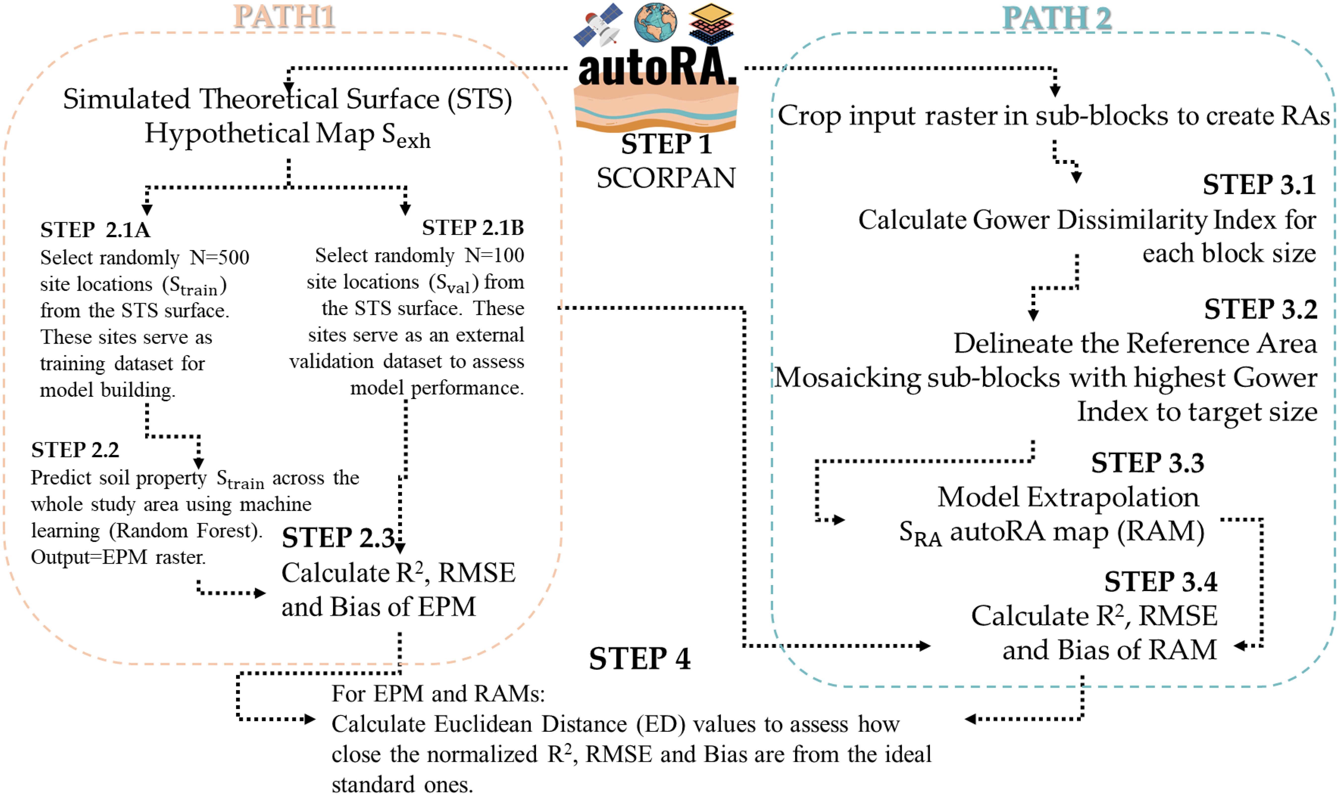
Figure 1. The workflow of the methodology (SCORPAN= Theoretical, quantitative model for soil modeling and mapping (1), S, Soil; C, Climate; O, Organisms including land cover and natural vegetation; R, Relief including terrain attributes; P, Parent material including lithology; A, Age/the time factor; and N space, spatial or geographic position; STS = Simulated Theoretical Surface; RMSE= Root Mean Squared Error; R² = Coefficient of Adjustment; EPM, Exhaustive Predicted Model; RAM, Reference Area Model Prediction for the target properties STS; RF, Random Forest. autoRA logo before STEP 1 (trademark number 937505684).

Path 2 involved computations of possible RAs via the sensitivity methodology entailing calculation of the Gower’s Dissimilarity Index, delineation of the RA boundaries, predictions of S_RA using machine learning (Random Forest) with various parameter settings of lower and upper bounds, validation of the various S_RA using an independent validation dataset, and model performance assessment (metrics: R², RMSE, and Bias).

Path 2 represents the part of the algorithm that effectively creates the RAs by cropping the input raster maps (blue border boxes on the right of Figure 1). It involved STEP 3.1, which calculated the Gower’s dissimilarity index for each covariate of the SCORPAN model loaded into autoRA, considering different block sizes. In STEP 3.2, the algorithm delineated the limits of the RAs by mosaicking the highest values ​​of the Gower’s dissimilarity index concerning the average Gower’s dissimilarity index of the full extension of the study area. In STEP 3.2, the algorithm created RAs with different dimensions (i.e., respecting the size of RAs inputted by the user on the parameter target area), represented in terms of % of the area relative to the full extension of the study area (10 to 50%, increasing at a 10% growth rate). STEP 3.3 used a fixed number of points sampled within each generated RA to build S_RA prediction models to be applied for the whole AOI. The prediction models are called Reference Area Model (RAM).

Results from Path 1 (i.e., the exhaustive benchmark, the EPM raster surface) and Path 2 (i.e., RAM raster surfaces for multiple RAs) were compared to each other using evaluation metrics (R², RMSE, and Bias) in STEP 4. To compare the metrics and choose the RA that produces the best model, the Euclidean Distance (ED) of the metrics of each RA with an idealized standard vector of these metrics was used (R² = 1, RMSE = 0, and Bias = 0). The RA with the smallest ED value concerning the standard vector was identified as the best-performing RA for a given study area.

2.2 Applying the autoRA in two contrasting soilscapes

2.2.1 The study sites

Two study areas were selected to evaluate the effectiveness of the autoRA algorithm in different pedological contexts characterized by different soil formation factors. The regions chosen are the State of Florida, located in the USA, with an area of 170,304 km², and the State of Rio de Janeiro in Brazil (BR), with an area of 43,653 km² (Figure 2). Florida is characterized by a predominantly flat terrain, with elevations ranging from sea level up to 110 m. The soil’s parent material mainly comprises marine sediments and limestone rocks, resulting in a geology dominated by sedimentary formations (27). The climate is mostly humid subtropical, with annual precipitation ranging between 1,200 mm and 1,800 mm, significantly influencing pedogenetic processes. The primary soil types in Florida are Spodosols with acidic spodic horizons and Entisols and Inceptisols. Ultisols, which are clayey soils that are intensely weathered, are present in regions with slightly elevated relief. Histosols, carbon-rich wetland soils, are prominent throughout Florida, occurring in the form of isolated wetlands and the Greater Everglades in South Florida (28). The main factors in soil formation in Florida include sedimentary material, hot and humid climate, moderate to high precipitation amounts, predominant vegetation of coniferous forests and coastal plains, and flat relief that favors slow drainage and accumulation of organic matter (29).

Figure 2

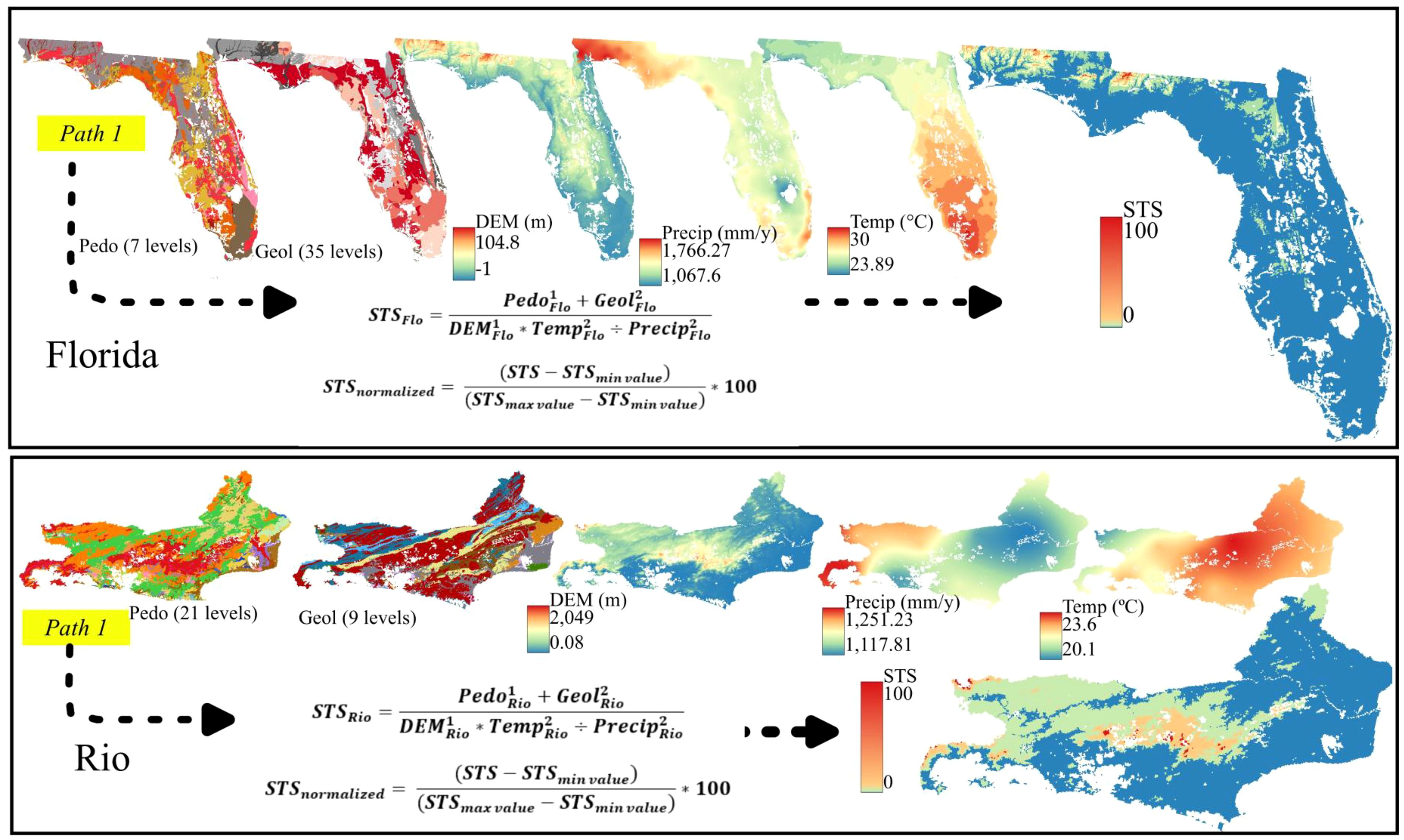
Figure 2. Raster stacking (Path 1) to calculate the STS for Florida and Rio de Janeiro. Pedo, Pedology; Geol, Geology; DEM, Digital elevation model (meters); Precip., Annual average precipitation in millimeters; Temp., Annual average temperature in °C.

The State of Rio de Janeiro has a complex geology composed of igneous and metamorphic rocks, such as granites and gneiss, associated with sedimentary rocks and colluvial and alluvial deposits (30). The relief is mountainous, with altitudes that reach 1,600 meters, as in the Serra dos Órgãos Mountains (Figure 3). The climate is humid tropical, with annual precipitation between 1,000 mm and 2,500 mm, influenced by the proximity of the Atlantic Ocean (31). The pedological diversity includes the majority occurrence of Oxisols, Inceptisols, and Ultisols (32). Soil formation factors in Rio de Janeiro are influenced by geological diversity, mountainous relief, humid climate, and dense vegetation of the Atlantic Forest, which contribute to the high rate of weathering and deep soil formation (33–35).

Figure 3

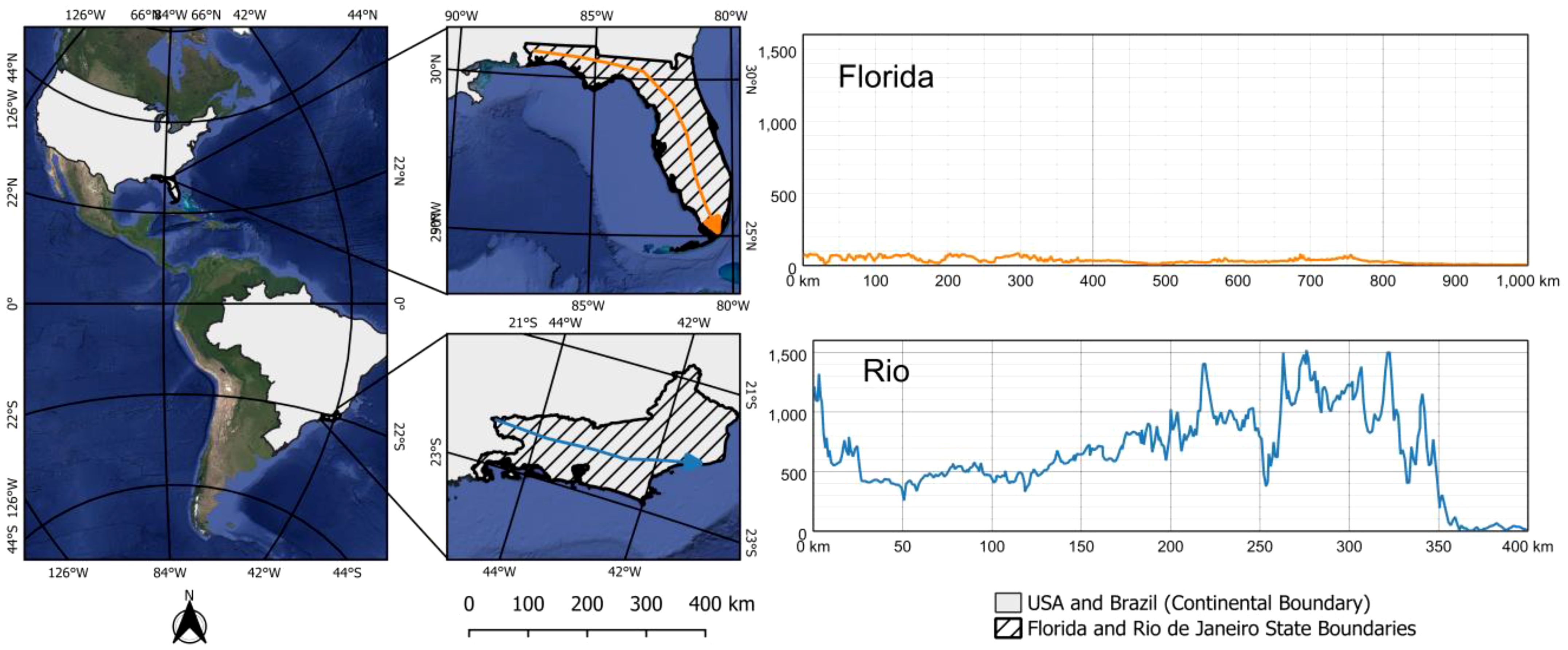
Figure 3. Location map of Florida and Rio de Janeiro and their respective elevation profiles.

2.2.2 The environmental covariates

To represent the soil formation factors (36), five environmental covariates were selected for each study area (STEP 1, Figure 1) to apply the autoRA algorithm and generate the STS (Path 1, Figure 1). The soil map provided by the Natural Resources Conservation Service (NRCS) (37) was used to identify the types of soils in Florida at a scale of 1:250,000, containing seven soil levels. The U.S. Geological Survey (38) the geologic map containing 35 geologic levels for the Florida region alone at a scale of 1:100,000 was made available. The relief was represented by a digital elevation model (DEM) with a resolution of 30 m and made available by the National Aeronautics and Space Administration using Advanced Spaceborne Thermal Emission and Reflection Radiometer satellite data. The raster data of average annual precipitation and average annual temperature from 1981 to 2010 were obtained from the PRISM Climate Group (39).

For Rio de Janeiro, the soil maps were made available by the Brazilian Institute of Geography and Statistics (32) at a scale of 1:250,000 containing 21 soil levels. The IBGE provided the geology map at a scale of 1:250,000 with nine geological levels. To represent the relief of Rio de Janeiro, the DEM of the Shuttle Radar Topography Mission (SRTM) satellite with a spatial resolution of 90 m was used. The precipitation and average annual temperature maps were obtained from the WorldClim database (40) with a spatial resolution of 1 km from 1980 to 2016. All covariates for both case studies were harmonized to 1 km spatial resolution.

2.2.3 The simulated theoretical surface

The STS (Path 1) in Figure 1 was implemented using an adapted methodology from Meyer and Pebesma (41). The STS acts as a hypothetical target variable (S_exh) that is both explainable and plausible, reflecting soil information derived from environmental covariates for a given study area. Before the map algebra, all categorical covariates (e.g., a geology map with multiple classes) were split into separate raster layers using dummy transformations of 0 or 1. Thus, each category becomes an individual map with presence coded as 1 and absence as 0. Numeric covariates, such as digital elevation models (DEM), precipitation, or temperature, were scaled to a 0–1 range to ensure comparability across all variables.

Using these standardized covariates, the STS is generated via map algebra interactions among the covariate maps (Figure 2), ensuring consistency with their spatial patterns. For example, the STS in Florida (STS_Flo) is computed by $ST{S}_{Flo}= Ped{o}_{Flo}+Ge{o}_{Flo}+(DE{M}_{Flo}* Preci{p}_{Flo})+ Tem{p}_{Flo}$, while the STS in Rio de Janeiro (STS_Rio) is calculated as $ST{S}_{Rio}= Ped{o}_{Rio}+Ge{o}_{Rio}+DE{M}_{Rio}+ (Preci{p}_{Rio}*Tem{p}_{Rio})$.

As a calculated synthetic map, the STS is assumed to be error-free. Figure 2 illustrates this process for both Florida and Rio de Janeiro. To facilitate direct comparison, each STS is subsequently normalized to a 0–1 scale using $ST{S}_{normalized}=\frac{STS-ST{S}_{min}}{ST{S}_{max}-ST{S}_{min}}$and then multiplied by 100 to yield a final scale from 0% to 100%. Because this map algebra product is solely an interaction of covariates, it does not represent a physically measured quantity. Instead, it is a spatially plausible synthetic surface that reflects the relative influence of each covariate on a hypothetical soil property. These dimensionless ${\text{STS}}_{\text{normalized}}$values serve as a reference populated with S_exh for all subsequent analyses, functioning as a benchmark map to assess the efficiency of parameters of the autoRA algorithm.

2.2.4 Training and validation datasets

A grid of 500 points (representing site locations) was randomly generated (STEP 2.1A). We chose a random distribution of these points to ensure adequate spatial representativeness and avoid excessive concentration in certain areas that could introduce biases in the predictive model. To allow side-by-side comparisons of Path 1 (EPM) and Path 2 (RAMs), the same number of points (N: 500) were chosen in each of the two study areas. We used the spatial extraction function in ArcGIS Pro to extract the variable S_train at the 500 site locations of STS_Flo and STS_Rio. The S_train values were then used as the target (dependent) variable for predictive model development using machine learning (training phase). A second grid of 100 points (representing site locations) was randomly extracted from the STS raster, with variable Sval serving as an external validation dataset in each study area (STEP 2.1B). An independent validation set is essential to verify the model’s ability to generalize its predictions to new samples not used during a model’s training, thus ensuring the reliability and applicability of the results obtained.

Figure 4 illustrates the spatial distribution of the training and validation points in both study areas (Florida and Rio de Janeiro). We used the Random Forest (RF) machine learning algorithm to develop predictive models using the environmental covariates of the SCORPAN model (pedology, geology, digital elevation model, average precipitation, and average temperature) as input (independent) variables and S_train as output (target) variable (STEP 2.2 of Path 1 in Figure 1). Training models were customized to study areas with separate RF training models developed for Florida and Rio. We employed the “randomForest” package (42) available for the R software (43).

Figure 4

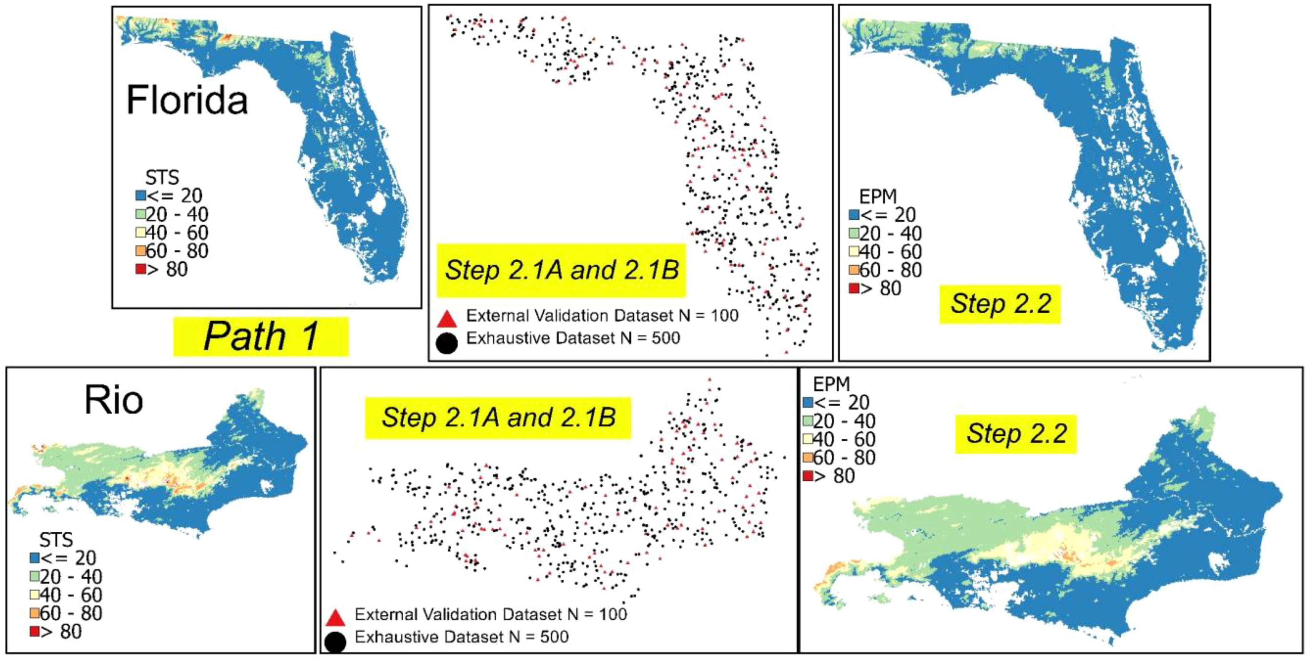
Figure 4. Spatial distribution of the training (N: 500) and validation (N: 100) datasets for the selected study areas. Path 1, Simulated Theoretical surface (STS); sampling training and validation dataset (STEP 2.1A and STEP 2.1B of Figure 1); Exhaustive Prediction Model (EPM) using the training dataset and Random Forest machine learning – STEP 2.2).

In our RF regression modeling for the Florida and Rio datasets, we employed the default parameters provided by the R package randomForest to ensure consistency and reliability across our analyses. Specifically, each model was constructed with 500 trees (ntree = 500), a number sufficient to ensure that every input row is predicted multiple times, thereby enhancing the stability and accuracy of the predictions. The number of variables randomly sampled as candidates at each split (mtry) was set to 1, following the default of one-third of the total predictors (p/3), given that each dataset contained five predictors. Additionally, the minimum size of terminal nodes (nodesize) was maintained at the default value of 5, encouraging the growth of smaller, more computationally efficient trees while preventing overfitting. By adhering to these default parameter settings for the Florida and Rio Random Forest regression models, we ensured a balanced approach that optimizes predictive performance and computational efficiency without requiring extensive parameter tuning.

The RF algorithm was chosen based on its ability to handle large volumes of data, its robustness in noisy data, and its ability to capture highly nonlinear relationships between the covariates and the dependent variable. In addition, RF offers internal validation mechanisms, such as estimating the importance of variables, which contribute to the interpretation and improvement of the model (44). The trained machine learning model for Florida using the S_exh generated the STS-EPM raster for Florida while the same procedure was used to create the STS-EPM for Rio de Janeiro.

2.2.5 Determining the Gower index and delineating the reference areas

In Path 2 (STEP 3.1 and 3.2 in Figure 1), the autoRA algorithm was run by cropping the Florida and Rio de Janeiro covariates and then calculating Gower’s dissimilarity index. The algorithm offers an argument called block size (block size) that is dependent on the original spatial resolution of a given input raster. The block size parameter allows the grouping of pixels into a window defined by the number of rows x columns of the block (e.g., 5 x 5 pixels = 25 pixels total in a block). For example, if the original resolution of the covariates is 1 km² and the block size is set to 5, each block will have a dimension of 5 km x 5 km. Then, considering each block size value, the entire set of covariates is clipped using the respective block size mask.

Figure 5 shows the schematic mask used to clip the set of covariates from the values used for escalating block size values from lower to upper bounds of 5, 10, 20, 30, 40, 50, 100, and 150 for Florida and Rio. As noted earlier, all covariates for both study areas had been harmonized to 1 km spatial resolution. Applying a block size value of 5 resulted in 5 km x 5 km blocks (total size of 25 km²); likewise, increased block size values generated larger blocks across the study areas aggregating the input data.

Figure 5

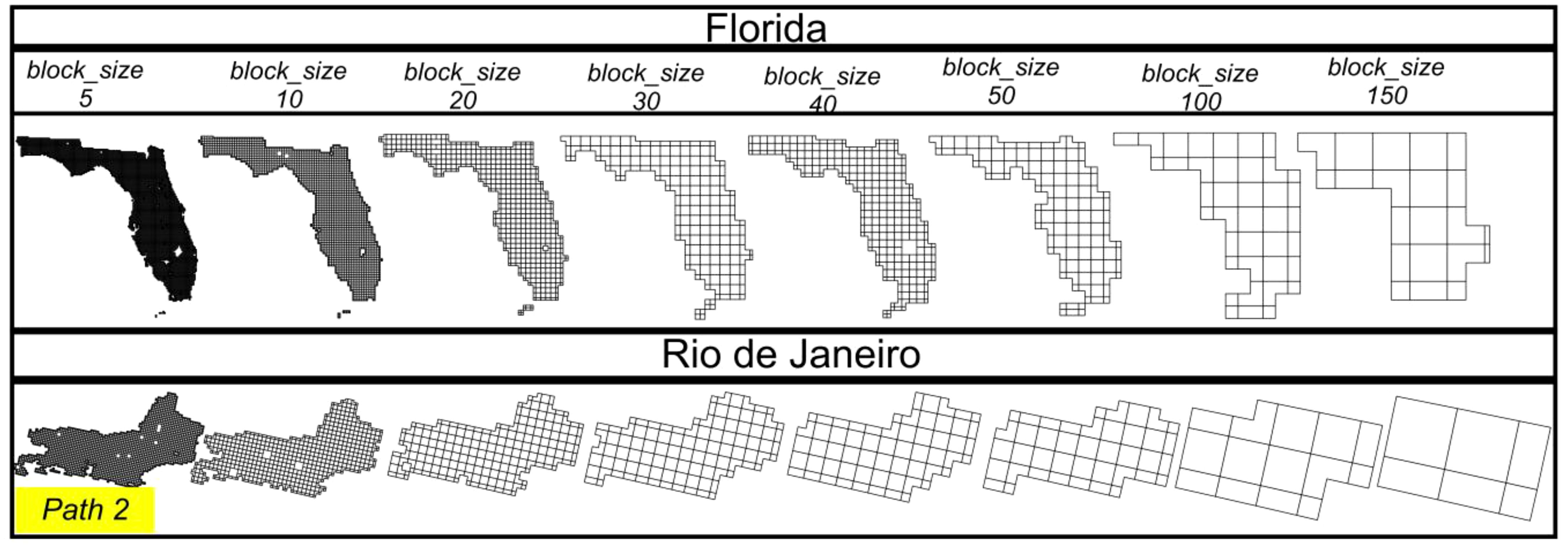
Figure 5. Block sizes and masks were used to calculate the Gower dissimilarity index in Florida and Rio de Janeiro (Path 2, STEP 3.1 of Figure 1).

The Gower’s dissimilarity index of the autoRA algorithms was calculated based on Gower (22) as described in Equations 1–3 (STEP 3.1 in Figure 1). Each block size value mask cropped a covariate raster, and the Gower’s dissimilarity index is calculated ($X_{block}$) and it was compared to Gower’s dissimilarity index of the covariate raster in the total area ($X_{total}$). Suppose the $X_{block}$values had a Gower’s dissimilarity index value close to the ($X_{total}$), it means that the dissimilarity is low with a value close to 0, and vice versa, it is high with a value close to 1.

This process is repeated for each covariate present in the data set. The dissimilarity values obtained for each covariable are then summed for each set of covariates grouped according to the size of the block size. The lower the sum of Gower’s dissimilarity indices for a given block size, the lower the diversity between the block investigated and the AOI. On the other hand, as the differences between the Gower indices calculated for each block and the AOI increase, the values tend to approach 1, indicating a high Gower’s dissimilarity index between the covariables in the specific pixel aggregation and the covariates of the entire area suggesting that the block captures significant variability that is not represented by the average value of the AOI.

$\begin{array}{ll}Gower Dissimilarit{y}_{block,total}=1-\frac{{\sum }_{k=1}^p{\delta }_k{d}_k}{{\sum }_{k=1}^p{\delta }_k}& (1)\end{array}$

Where $\text{p}$represents the total number of variables considered (e.g., geology, pedology, DEM, precipitation, temperature), and ${\text{δ}}_{\text{k}}$​ is an indicator that takes the value 1 if the variable $\text{k}$is valid for the comparison (i.e., relevant and has data available) and 0 otherwise. The term ${\text{d}}_{\text{k}}$is the normalized difference for variable $\text{k}$, which quantifies the dissimilarity between the block and the total area for that specific variable. The numerator sums the contributions of valid variables (${\text{δ}}_{\text{k}}{\text{d}}_{\text{k}}$​), while the denominator ensures that only valid variables are included in the normalization. The final value is subtracted from 1 so that the index represents dissimilarity, where higher values indicate greater dissimilarity between the block and the total area.

For numerical variables, such as temperature, precipitation, or elevation, ${\text{d}}_{\text{k}}$​ is calculated as the normalized difference between the block’s value (${\text{x}}_{\text{block},\text{k}}$​) and the total area’s value (${\text{x}}_{\text{total},\text{k}}$​). Here, (${\text{x}}_{\text{block},\text{k}}$​)​ represents the average or representative value of a variable $\text{k}$within the block, and (.​)​ represents the average or representative value of the same variable across the total area. These values, ${\text{x}}_{\text{block},\text{k}}$​ and ${\text{x}}_{\text{total},\text{k}}$​ are derived by calculating the average of the variable within the block or across the total area respectively. The normalized difference is computed by Equation 2​, where ${\text{Range}}_{\text{k}}$​ is the difference between the maximum and minimum values of $\text{k}$in the dataset.

$\begin{array}{ll}{d}_k=\frac{\left|x_{block,k}-x_{total,k}\right|}{Rang{e}_k}& (2)\end{array}$

Equation 3 defines the values of ${\text{d}}_{\text{k}}$in case of categorical variables, such as the maps of geology and pedology.

$\begin{array}{ll}{d}_k=\{\begin{array}{c}0, if x_{block,k} =x_{total,k}\\ 1, if x_{block,k} \ne x_{total,k}\end{array}& (3)\end{array}$

Another argument the autoRA algorithm has is the target area, which represents the size of the RA that the user would like to delineate. The pixel Gower values with the highest dissimilarity values (closest to 1) are grouped together to represent the user-desired ratio. This step of the autoRA algorithm describes STEP 3.2 (Figure 1). The target area argument allows the user to enter a list of percentage values. We selected the area ratios of 10%, 20%, 30%, 40% and 50% for the sensitivity analysis to demonstrate the behavior of target area on soil predictions (S_RA).

The search process iterates through various block size values used to calculate the Gower dissimilarity index. For instance, it might start with a larger grouping like 100 × 100 pixels. At this coarser resolution, the smoothed dissimilarity values reveal broad spatial patterns. In contrast, using a smaller block size such as 5 × 5 pixels produces a more detailed, fine-resolution map of Gower dissimilarity.

The autoRA algorithm systematically explores different area sizes by cycling through all values provided in the block size parameter. For example, if the target area is set to 10%, the algorithm applies the same pixel grouping defined by the block size. It then increases the target area to 20% and repeats the process, continuing this pattern until all specified block size and target area values have been used. As a result, the algorithm generates multiple RA formats by combining each target area value with each block size. This approach allows autoRA to capture a range of spatial patterns at different resolutions and area sizes.

2.2.6 Prediction and accuracy of modeling the exhaustive and reference area dataset

According to Path 1, the autoRA algorithm used 500 points extracting dimensionless values from the STS for each x and y coordinate, allowing the building of the benchmark model EPM that covered the full extension of the AOI. The same number of points (N: 500) were also selected in Path 2 to model soil property S_RA for each RA (STEP 3.3 in Figure 1). We used the conditioned Latin hypercube sampling method (16) with the maps of pedology, geology, temperature, precipitation, and the digital elevation model as inputs to place the 500 site locations for each of the two study areas (Florida and Rio de Janeiro). Random Forest machine learning was used for training prediction models at the 500 sites with covariates as inputs and S_RA as output. Separate RF models were created for each of the study areas. Finally, these models were upscaled to the entire Florida and Rio de Janeiro study region, creating RAM rasters.

We used autoRA to validate the EPM and RAM rasters created in STEP 2.3 of Path 1 and STEP 3.4 of Path 2, respectively. The same independent validation dataset (N: 100) identified in STEP 2.1 B of Path 1 was used to assess EPM and RAM via external validation. The metrics used to evaluate accuracy were the Root of Mean Squared Error (RMSE) and Bias, and the Adjusted Coefficient of Determination (R²) was used to quantify the model fit.

The RMSE (Equation 4) measures the average magnitude of the errors between predicted and observed values; hence, values close to 0 indicate better model accuracy. Bias (Equation 5) quantifies the systematic error in the prediction over an external validation dataset, representing the average difference between the predicted and observed values. A Bias value close to zero indicates the absence of a systematic trend during the adjustment of the prediction model. The R² (Equation 6) means the proportion of variance in the training dataset that the model explains. Values close to 1 indicate that the adjusted model has a high explanatory capacity.

$\begin{array}{ll}\text{RMSE}=\sqrt{\frac{1}{n}\sum _{i=1}^n{(y_i-\widehat{y_i})}^2}& (4)\end{array}$

$\begin{array}{ll}\text{Bias}=\frac{1}{n}\sum _{i=1}^n(\widehat{y_i}-y_i)& (5)\end{array}$

$\begin{array}{ll}{\text{Adjusted R}}^2=1-\frac{{\sum }_{i=1}^n(y_i-\widehat{y_i})}{{\sum }_{i=1}^n(y_i-\overline{y})}& (6)\end{array}$

Where ${\text{y}}_{\text{I}}$are the values of the target variable simulated surface extracted for each of the 100 points intended for the composition of the dataset for external validation; $\widehat{{\text{y}}_{\text{I}}}$are the simulated surface values predicted for the 100 external validation points from the prediction models for each combination of tested arguments such as block size and target area size; $\overline{\text{y}}$is the average of the 100 observed simulated surface values for the external validation group; $\text{n}$is the number of observations present in the validation set.

The Euclidean Distance (ED) was calculated to synthesize the metrics presented in Equations 4–6. To calculate the Euclidean distance of the RMSE, Bias, and Adjusted R² metrics, it was essential to first scale them. Normalization ensures that all metrics contribute equally to the distance calculation, regardless of their original units or ranges. The escalation considered the maximum and minimum values present among all combinations of target area and block size used. Equations 7–9 were used to normalize the RMSE, Bias, and R², respectively.

$\begin{array}{ll}{\text{RMSE}}_{\text{normalized}}=\frac{\text{RMSE}-\text{minimum}(\text{RMSE})}{\text{maximum}(\text{RMSE})-\text{minimum}(\text{RMSE})}& (7)\end{array}$

$\begin{array}{ll}{\text{Bias}}_{\text{normalized}}=\frac{\text{Bias}-\text{minimum}(\text{Bias})}{\text{maximum}(\text{Bias})-\text{minimum}(\text{Bias})}& (8)\end{array}$

$\begin{array}{ll}{\text{R}}^2\text{normalized}=\frac{{\text{R}}^2-\text{minimum}({\text{R}}^2)}{\text{maximum}({\text{R}}^2)-\text{minimum}({\text{R}}^2)}& (9)\end{array}$

The ED was calculated to assess how close the normalized values are to the ideal standard ones: RMSE = 0, Bias = 0, and R² = 1. From the normalized RMSE, Bias, and R² values, the distances were calculated using Equation 10. A lower ED value indicates that the metrics are closer to the ideal values, suggesting a more accurate and less skewed model. In contrast, higher distance values signal a more significant discrepancy between the standard values.

$\begin{array}{ll}\text{Euclidian Distance}=\sqrt{{(0-\text{RMSE})}^2+{(0-\text{Bias})}^2+{(1-{\text{R}}^2)}^2}& (10)\end{array}$

2.3 Cost simulations

We conducted a cost simulation to assess the practical efficiency of the autoRA algorithm. This simulation considered standard parameters influencing sampling logistics costs and planning during fieldwork. Specifically, the daily road mileage required to reach each sampling coordinate, the salaries of the necessary personnel, and the number of days needed to complete the sampling project were a product of the calculus between the road length required to reach all the points and the maximum distance threshold to be driven by day. We applied the EPM sampling cost simulation utilizing the whole length of the road network made available for the State of Florida (45) and the State of Rio de Janeiro (32). The road network for both study areas is shown in Figure 6.

Figure 6

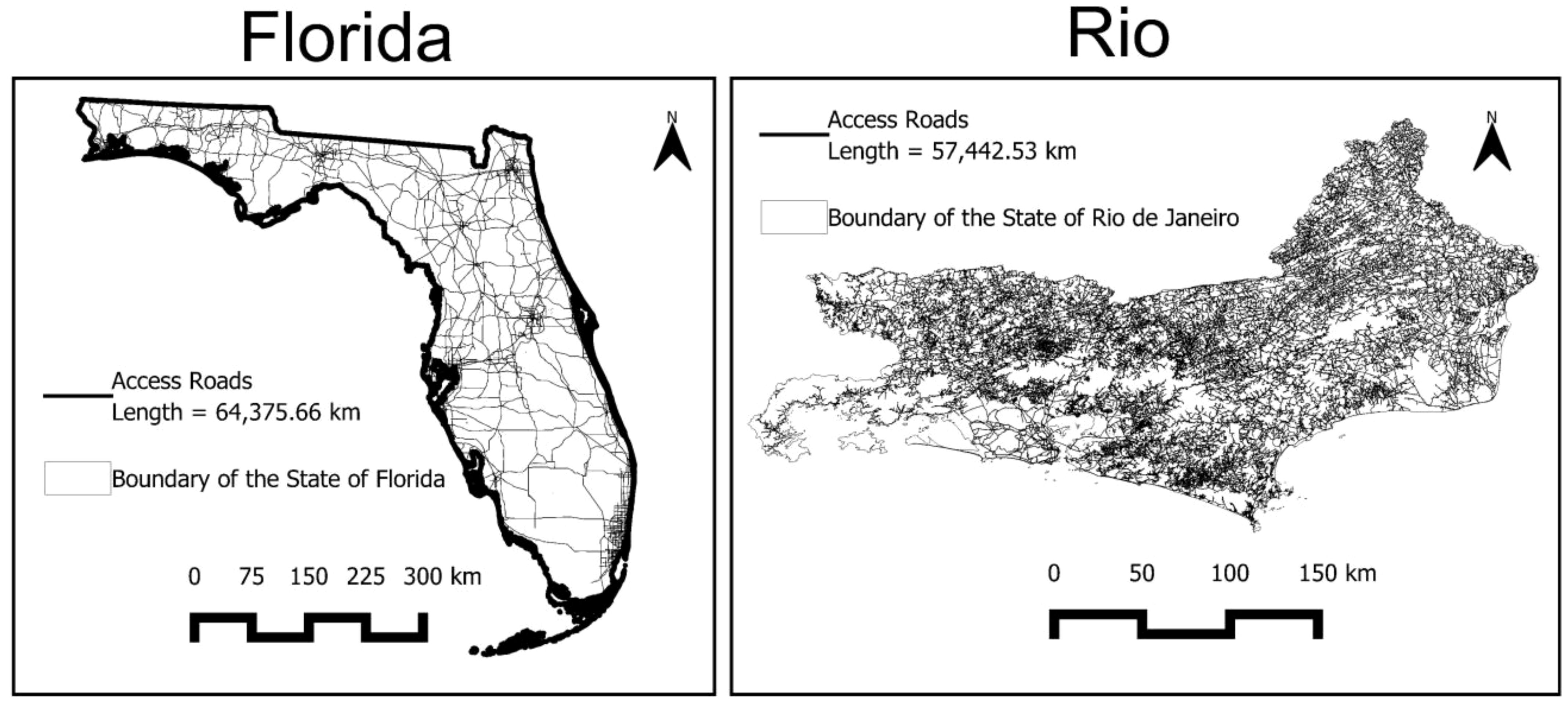
Figure 6. Main access roads for the states of Florida and Rio de Janeiro.

For the RAMs created from the dataset within each delineated RA from each combination of target area and block size, the shape of the roads was clipped using the respective RA extension as a mask to retain the roads inside it. The fuel cost was estimated at US $0.50 per kilometer traveled, with a maximum daily travel limit of 150 km. A Field Technician was considered to receive a salary of US $200 per day each.

3 Results and discussion

3.1 Gower’s dissimilarity index by block size

Results of the effect of varying block sizes on Gower dissimilarity index values were evaluated for Florida (USA) and Rio de Janeiro (Brazil). Different block sizes in the autoRA generate clipping masks from the covariate maps, influencing the aggregation of pixel values and the resulting Gower’s Dissimilarity values. As the block size value increases, spatial variability has a progressive aggregation and smoothing effect. This results in more generalized representations of Gower’s dissimilarity values. Smaller block sizes (e.g., 5, 10) retain detailed spatial variability, whereas larger block sizes (e.g., 100, 150) smooth out these variations, emphasizing broader spatial patterns. Consequently, higher block sizes obscure local-scale variability, presenting a more homogeneous view of dissimilarity across the study areas (Figure 7).

Figure 7

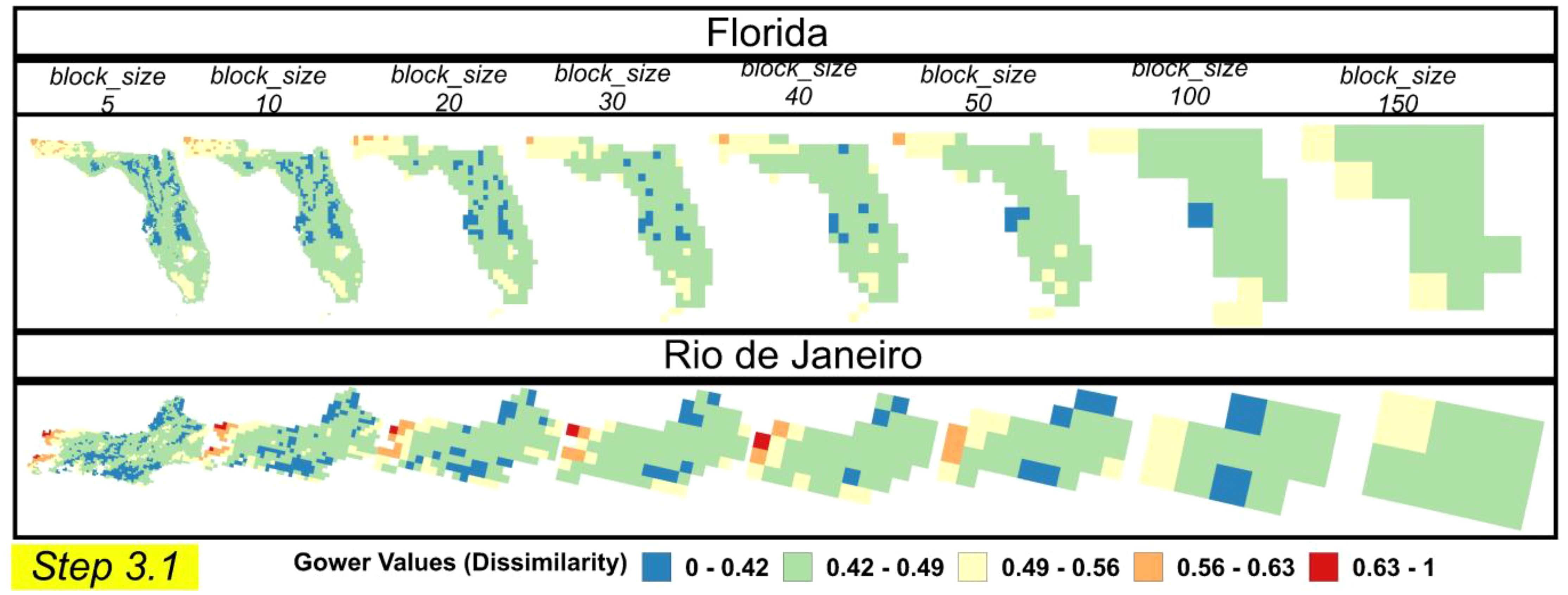
Figure 7. Gower’s dissimilarities index map for block sizes and two study areas (Florida and Rio de Janeiro). A range of 5 classes is applied.

The Gower’s Dissimilarity Index values across both regions range from 0.42 to > 0.63, with maps and a unified legend scale for direct comparison, as shown in Figure 7. In Florida, the highest Gower values (0.56–0.63) are primarily concentrated in the northwest region, mainly when smaller block sizes (5–30) are used. These areas become less distinct with larger block sizes (≥ 50) due to spatial smoothing.

In Rio de Janeiro, the city’s western region records the highest Gower’s Dissimilarity Index values, ranging between 0.56 and 0.63. This elevated dissimilarity coincides with Rio de Janeiro’s prominent mountainous landscape, notably including Agulhas Negras Peak, which soars to 2,800 meters and is located within the protected Itatiaia National Park. The western and mountainous areas on Rio de Janeiro were reported as the most dissimilar by Elias et al. (46) when they classified the state of Rio de Janeiro with dissimilar areas using a threshold of 0.34 of the Gower’s Dissimilarity Index.

3.2 Reference areas’ spatial distribution by block size and target values

Results from the implementation of STEP 3.2 delineating a variety of RAs within lower and upper bounds of block size and target area are shown in Figure 8. These findings offer a comprehensive perspective on how spatial resolution (block size) and coverage (target area) interact to influence RA delineation and sampling efficiency. For smaller target areas such as 5, 10, 20, and 30%, the delineation of the RA benefits from higher-resolution Gower’s Dissimilarity Index values, as evident in the first row of Figure 8 (Florida) and Figure 9 (Rio de Janeiro). In these scenarios, finer block sizes highlight subtle physiographic gradients, producing more intricately defined RA boundaries and enabling a more detailed, granular representation of environmental heterogeneity.

Figure 8

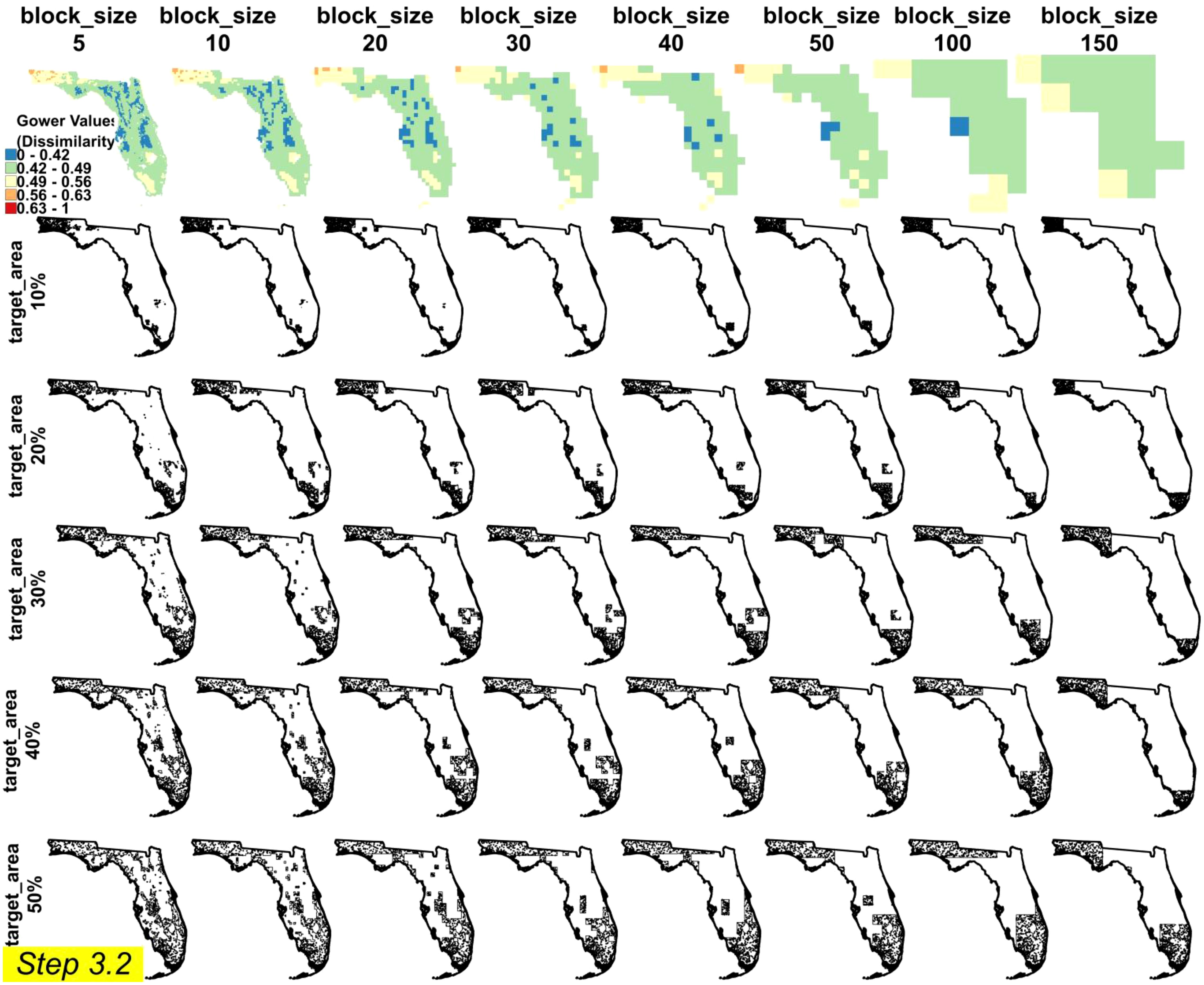
Figure 8. Delimitation of the reference areas (STEP 3.2) and placement of the training points within each reference area for Florida. Combinations of block size (rows) and target area (column) are shown. A range of 5 classes is applied.

Figure 9

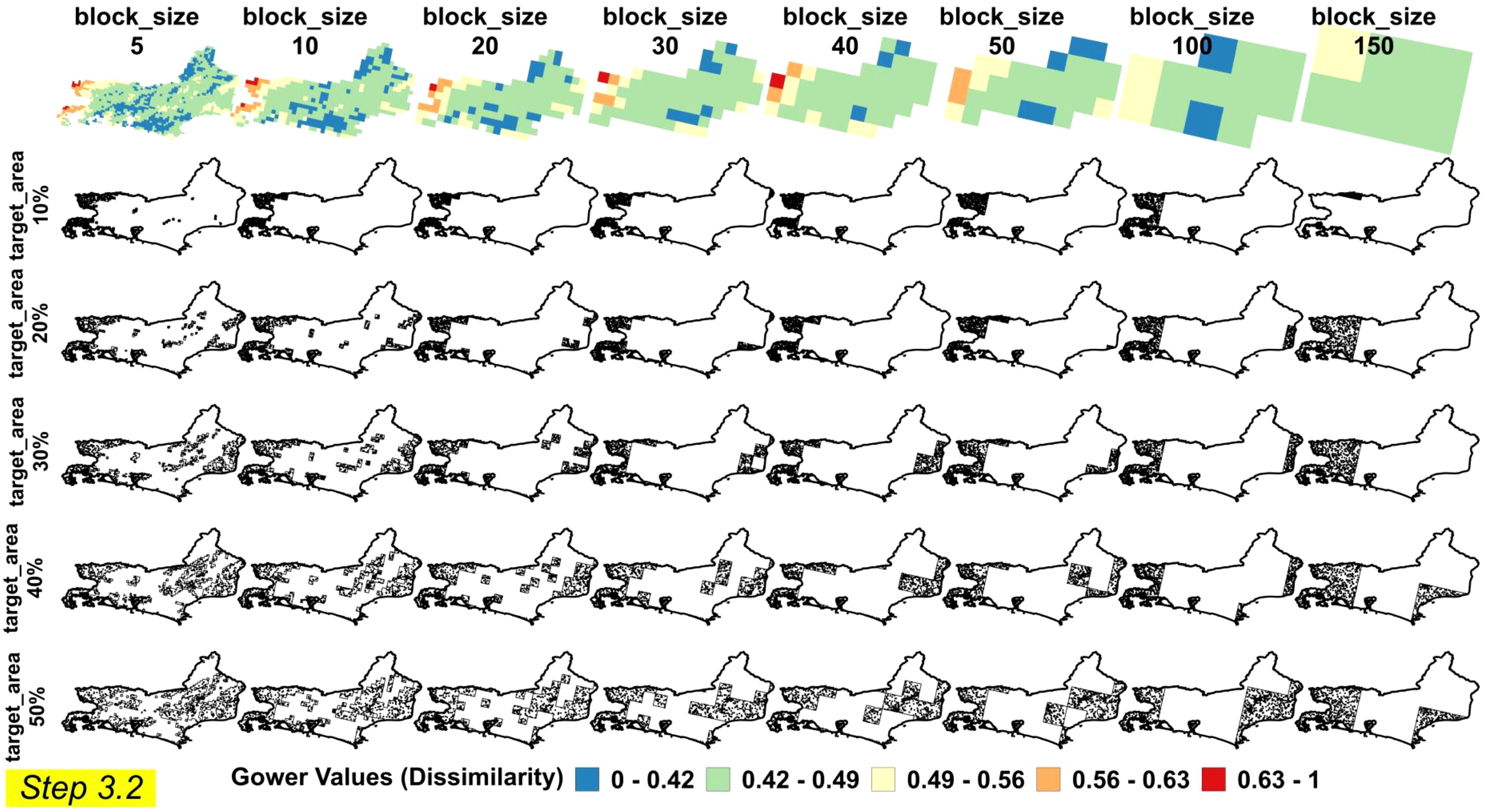
Figure 9. Delimitation of the reference areas (STEP 3.2) and placement of the training points within each reference area for Rio de Janeiro. Block size (rows) and target area (column) are combined. A range of 5 classes is applied.

As the target area increases to 40% and 50%, the delineated RAs encompass a broader range of physiographic information, effectively approaching the modal conditions of the entire region. The autoRA algorithm’s ability to scale from finer resolutions (yielding more detailed boundaries and subtle distinctions) to broader coverage (capturing widespread physiographic features) sets it apart from existing methods like CLAPAS and conditioned Latin Hypercube Sampling (cLHS). Unlike CLAPAS, which requires manual input of candidate RAs and lacks full automation, autoRA systematically evaluates environmental variability through Gower’s dissimilarity index, enabling a more holistic and flexible approach to RA delineation (14). Additionally, while cLHS ensures broad initial coverage, it does not dynamically adjust to the spatial heterogeneity of the landscape, potentially leading to redundant sampling or missed environmental gradients (2, 16).

As the RA encapsulates the more diverse soil-forming factor represented by the environmental variables used as input on the autoRA algorithm, the 500 training points within each RA are exhibited in Figures 8, 9 and are expected to perform the prediction of the STS by the RAM as well as the EPM. By doing so, autoRA enhances the scalability and efficiency of DSM workflows, particularly in diverse and challenging landscapes like those in Florida and Rio de Janeiro. This adaptability is essential for DSM practitioners seeking to optimize sampling designs in regions where traditional exhaustive sampling is neither feasible nor cost-effective (47, 48).

3.3 Reference area selection based on metrics and cost

Finding the optimized RA parameters was fundamental to ensuring the accuracy and efficiency of our RAM predictive models after testing several combinations of target areas and block sizes. This section presents a detailed analysis of various RA configurations based on key performance metrics – R², RMSE, and Bias – and incorporates the Euclidean Distance (ED) metric alongside cost simulations to guide the selection process. These configuration results are compared to EPMs, which served as our benchmark by sampling the entire study areas. It’s important to remember that all the R², RMSE, and Bias in Figure 10 are presented in a scale format (varying from 0 to 1) so they can be compared with the benchmark metric values.

Figure 10

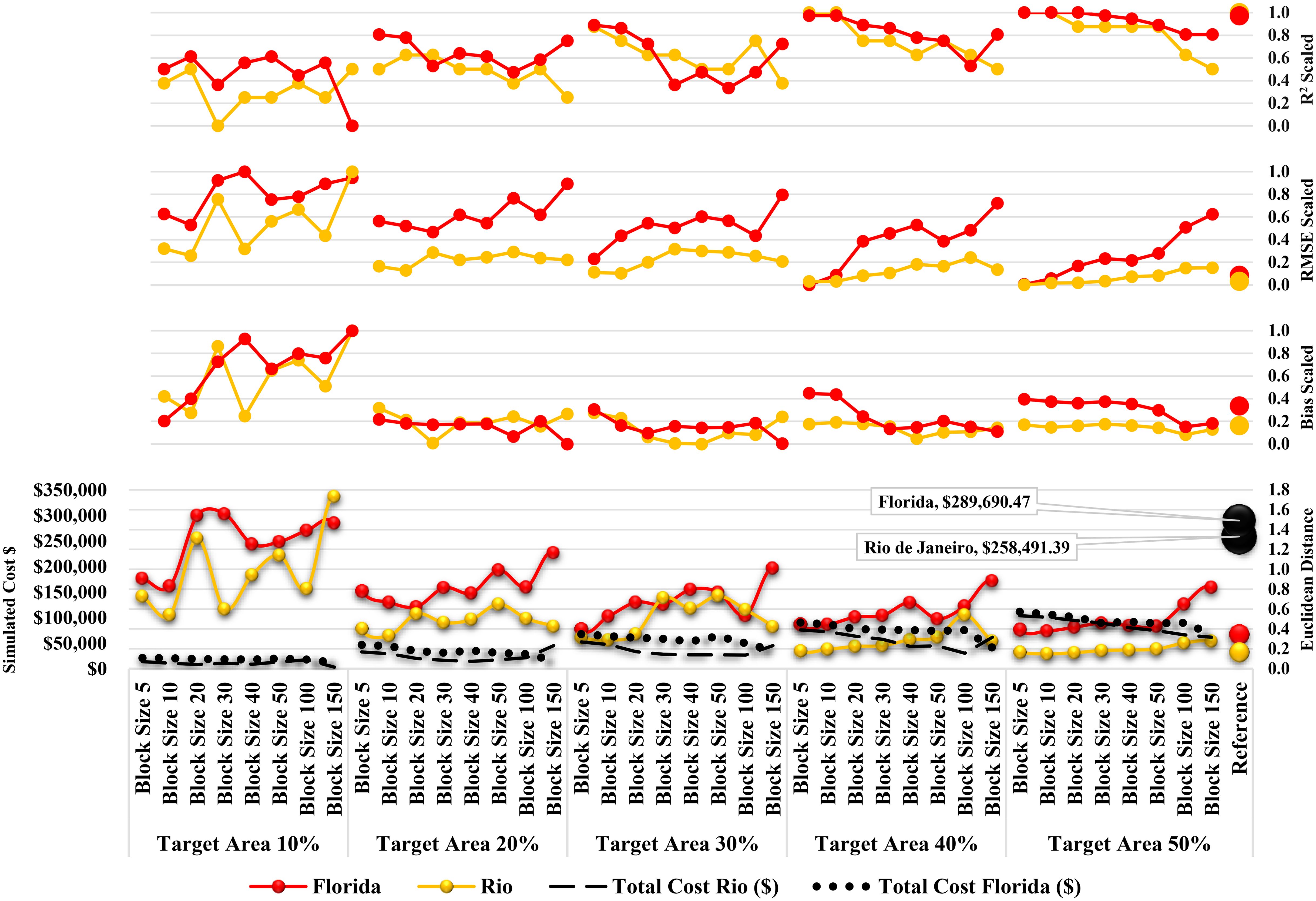
Figure 10. Metrics R², RMSE, Bias, ED, and simulated cost for each combination of the target area and block size for the autoRA’s configuration for Florida and Rio de Janeiro.

In Figure 10, larger target area sizes consistently exhibit higher R² values, demonstrating enhanced explanatory and model fit compared to smaller target area values. For instance, the RAM 50% target area size achieves the highest R², closely approaching the EPM benchmark model’s performance. The RMSE assesses the average magnitude of prediction errors, with lower values signifying more accurate predictions. Figure 10 shows a clear trend where larger target areas yield lower RMSE values, indicating improved prediction precision. The RAM 50% target area size records the lowest RMSE, suggesting that increasing the target area size significantly reduces prediction errors. The Bias measures systematic errors in predictions, reflecting whether the model overestimates or underestimates the observed values. A Bias value close to zero is desirable, as it indicates systematic minimal misprediction. The analysis reveals that larger target areas tend to have Bias values nearer to zero, highlighting their capability to provide more balanced and unbiased predictions. For example, the 40% and 50% target area sizes exhibit the smallest Bias values, underscoring their reliability for predicting accurately outside the RA-delineated boundaries.

The ED results (Figure 10) calculated for each RAM demonstrated a decreasing trend as the target area size increased. However, costs also rose because a larger target area encompassed more roads and required more time to drive to all recommended sampling points. The ED results using the RA approach were notably similar for Florida and Rio de Janeiro. The smallest ED values for RAM were 0.38 and 0.15, respectively, achieved with a target area of 50% and a block size of 10. The EPM benchmark model showed slightly lower ED values of 0.35 for Florida and 0.17 for Rio de Janeiro. The slightly higher metric of the ED compared to the Rio’s could be addressed by the randomization process of sampling the 500-training dataset for the EPM.

By limiting the sampling to 50% of the total study area for Florida and Rio de Janeiro, the RAM approach resulted in a total cost reduction of approximately $110,000 compared to the EPM approach. The traditional EPM strategy incurred costs of $258,491 for Rio de Janeiro and $289,690 for Florida. In this way, when the RAM provided by autoRA with a target area of 50% and a block size of 10 represents a cost reduction of approximately 57% for Rio de Janeiro and 62% for Florida, highlighting the financial efficiency of the RA approach supported by the autoRA automation.

Consequently, the following results and discussion on the paper will focus on the block size of 10 and the target area of 50%, as these parameters yield the lowest ED values. Figure 11 presents the final outlined RAs for Florida and Rio de Janeiro. The access roads and sampling points within the RA are also overlayed in Figure 11.

Figure 11

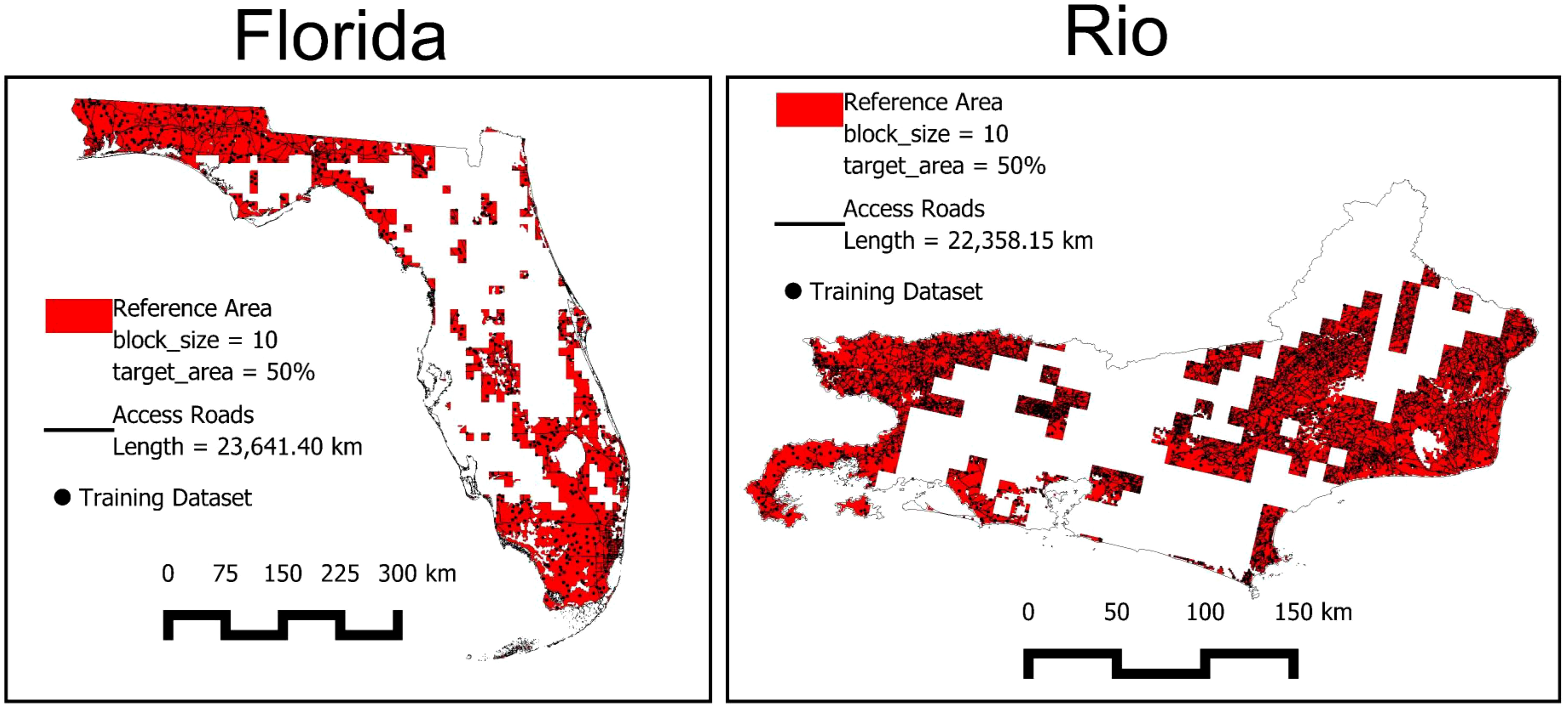
Figure 11. The Reference Area block size = 10 and target area 50% chosen for Florida and Rio, and the soil sampling placement of the training dataset (N: 500).

3.3.1 Florida reference area and predicted simulated theoretical surface analysis

Figure 12 displays the masked covariate maps for Florida’s delineated RAM, generated using the autoRA algorithm with a target area of 50% and a block size of 10. These maps illustrate how the autoRA algorithm retrieves the variability of key SCORPAN factors – parent material (Geol), soil type (Pedo), elevation (DEM), precipitation, and temperature – across the state.

Figure 12

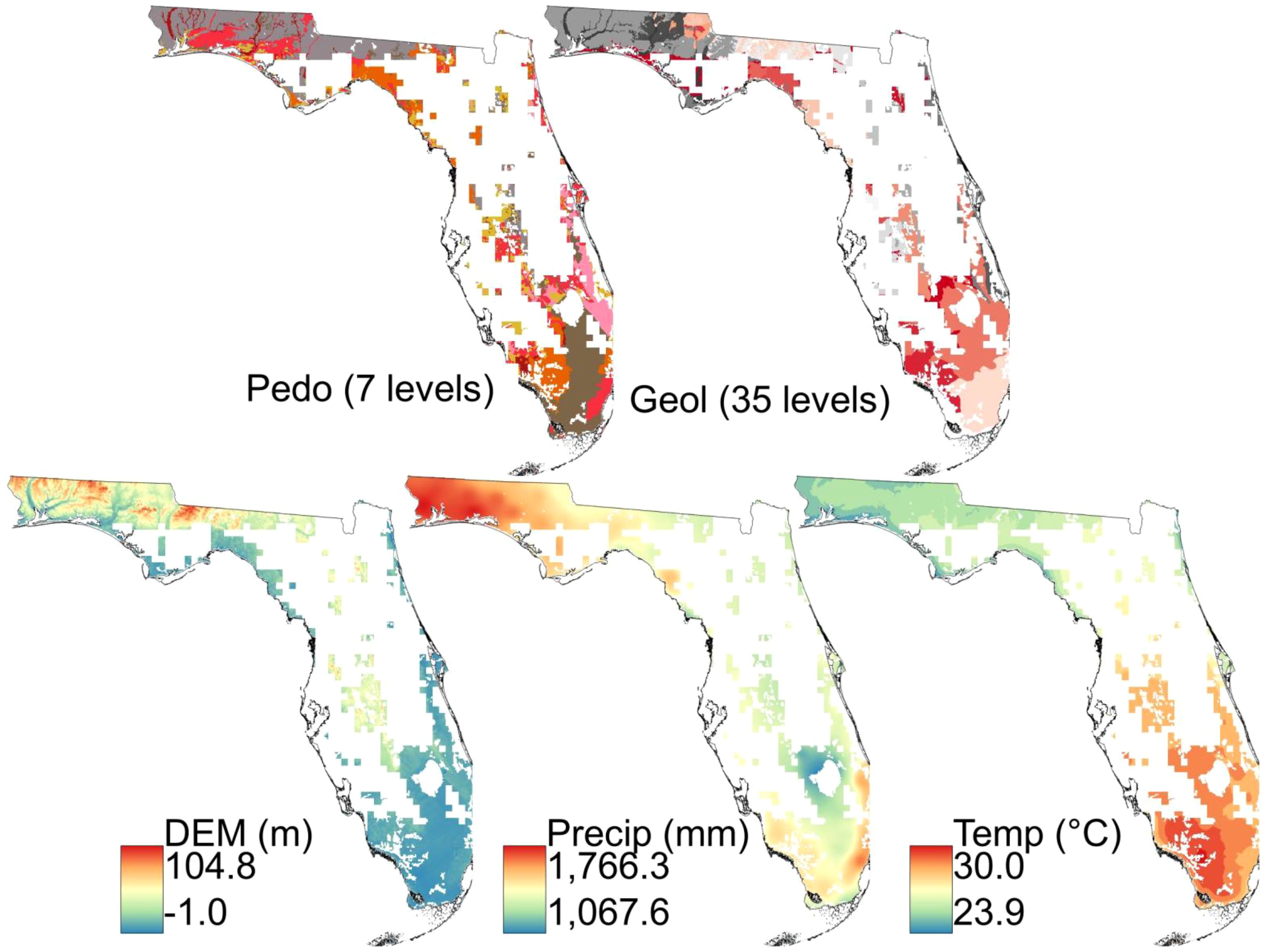
Figure 12. Covariables cropped for Florida’s reference area, with a block size of 10 and a target area of 50% delineated by the autoRA.

Regions dominated by sandy Entisols in well-drained uplands and coastal dunes, such as those captured in the Geol and Pedo maps, contrast sharply with the organic-rich Histosols in the poorly drained Everglades wetland soils in southern Florida. Similarly, the DEM map highlights low-relief areas associated with wetland hydrology and flatwood systems. In contrast, the precipitation and temperature maps emphasize climatic gradients that influence soil development across the state. These masked covariate maps demonstrate the algorithm’s ability to prioritize areas with diverse SCORPAN factor interactions while preserving spatial coherence.

Temperature variability in the RAM aligns closely with the EPM, with near-identical frequency distributions across the temperature range, ensuring that climatic gradients influencing soil formation are adequately captured (Figure 13). The precipitation distribution also reflects strong alignment, indicating that both drier and wetter regions are well-represented, which is crucial for capturing hydrologically driven soil patterns. Elevation variability is similarly preserved, with the RAM accurately reflecting the low-lying and upland areas characteristic of Florida’s topography, though minor underrepresentation is noted in the higher elevations. Figure 14 demonstrates the maps for the STS predicted for Florida using the RAM with the lowest ED metric from the combination target area of 50% and block size 10 and compares its spatial SPS distribution with the SPS map predicted by the sampling strategy of the EPM that worked as the benchmark map.

Figure 13

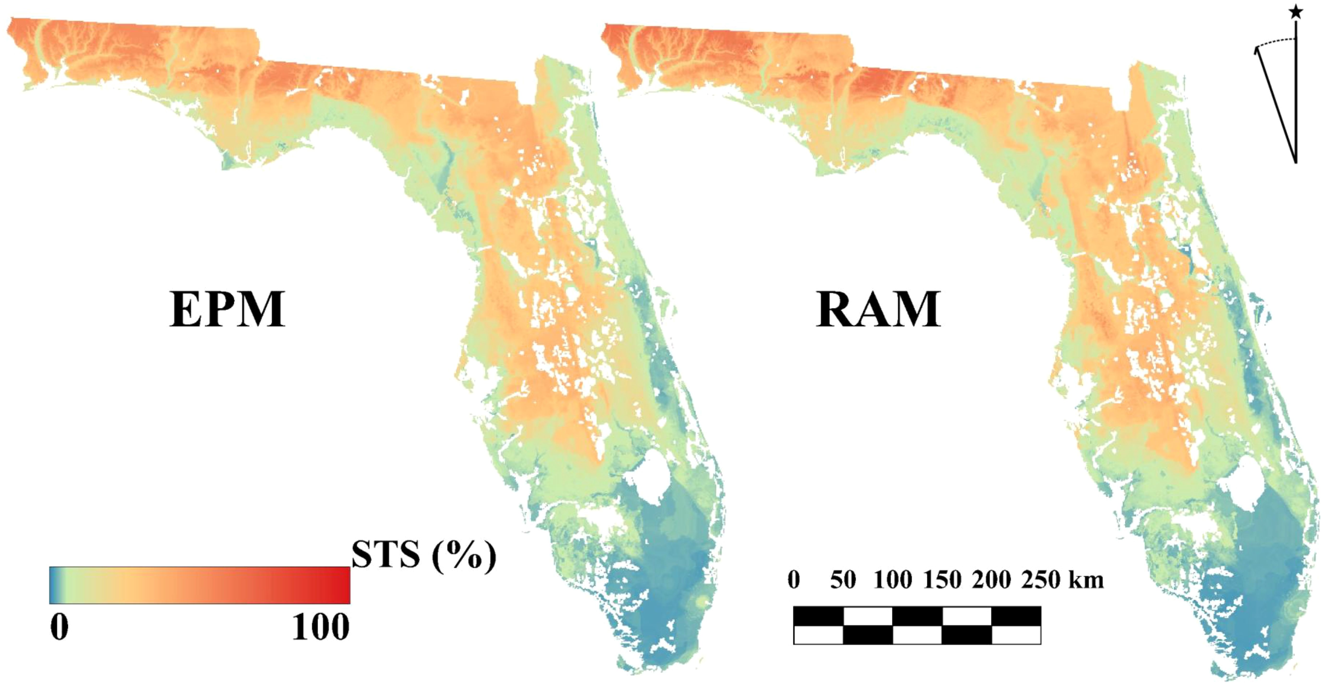
Figure 13. Comparison for the predicted Simulated Theoretical Surface (STS) maps via Exhaustive Prediction Model (EPM) using the whole area sampling strategy and Reference Area Model (RAM) using autoRA best Euclidean Distance metric for Florida.

Figure 14

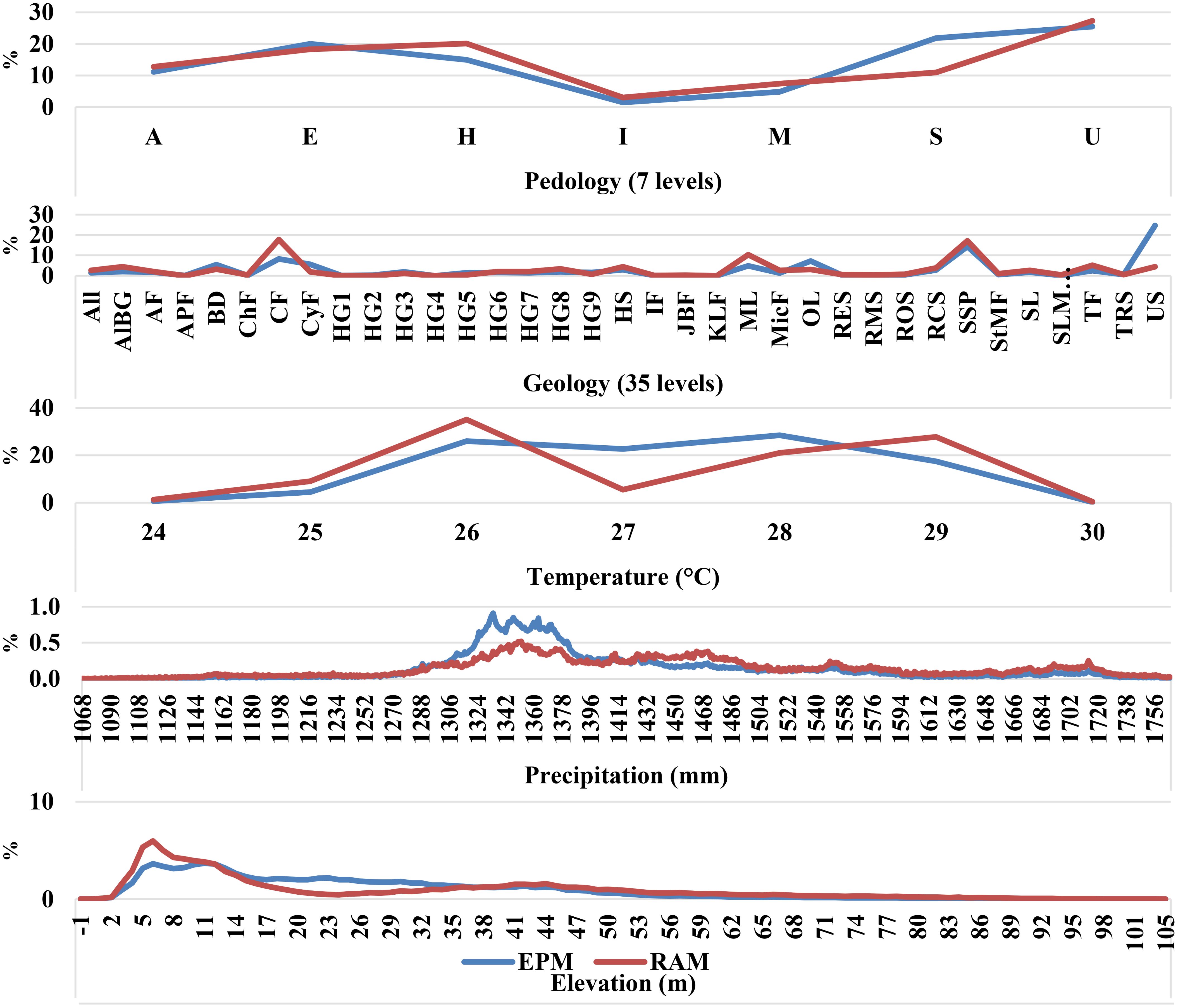
Figure 14. Frequency of pixel information for Exhaustive Prediction Model (EPM) and Reference Area Model (RAM). Pedology map: A, Alfisols; E, Entisols; H, Histosols; I, Inceptisols; M, Mollisols; S, Spodosols; U, Ultisols Geology map: All, Alluvium; AlBG, Alum Bluff Group; AF, Anastasia Formation; APF, Avon Park Formation; BD, Beach ridge and dune; ChF, Chattahoochee Formation; CF, Citronelle Formation; CyF, Cypresshead Formation; HG1, Hawthorn Group, Arcadia Formation; HG2, Hawthorn Group, Arcadia Formation, Tampa Member; HG3, Hawthorn Group, Coosawhatchie Formation; HG4, Hawthorn Group, Coosawhatchie Formation, Charlton Member; HG5, Hawthorn Group, Peace River Formation; HG6, Hawthorn Group, Peace River Formation, Bone Valley Member; HG7, Hawthorn Group, Statenville Formation; HG8, Hawthorn Group, Torreya Formation; HG9, Hawthorn Group, Undifferentiated; HS, Holocene sediments; IF, Intracoastal Formation; JBF, Jackson Bluff Formation; KLF, Key Largo Limestone; ML, Miami Limestone; MicF, Miccosukee Formation; OL Ocala Limestone; RES, Residuum on Eocene sediments; RMS, Residuum on Miocene sediments; ROS, Residuum on Oligocene sediments; RCS, Reworked Cypresshead sediments; SSP, Shelly sediments of Plio-Pleistocene age; StMF, St Marks Formation; SL, Suwannee Limestone; SLMLU, Suwannee Limestone-Marianna Limestone undifferentiated; TF, Tamiami Formation; TRS, Trail Ridge sands; US, Undifferentiated sediments.

Figure 14 demonstrates the percentage frequency of pixel values retrieved in the masked covariate maps, comparing the RAM-encapsulated pixels selected with the lowest ED (target area 50% and block size 10) to the EPM pixel for the whole study area of Florida. The results show that RAM effectively represents the variability of all covariates, ensuring that the selected RA encompasses the diversity observed in the entire dataset. For pedology, RAM preserves the distribution of dominant classes, such as Entisols and Spodosols, while also including less frequent classes, like Histosols, reflecting comprehensive soil variability. Similarly, geological variability is well-represented, with central lithological units such as Holocene sediments and residuum included, although minor deviations are observed for specific formations like the Hawthorn Group.

3.3.2 Rio de Janeiro reference area and predicted simulated theoretical surface analysis

The delineation of RA with the target area of 50% and block size 10 provided the lowest ED metric for Rio de Janeiro and its respective masked covariate maps are shown in Figure 15. The masked maps of pedology, geology, elevation, precipitation, and temperature illustrate how the RA prioritizes regions with distinct soil-forming factors.

Figure 15

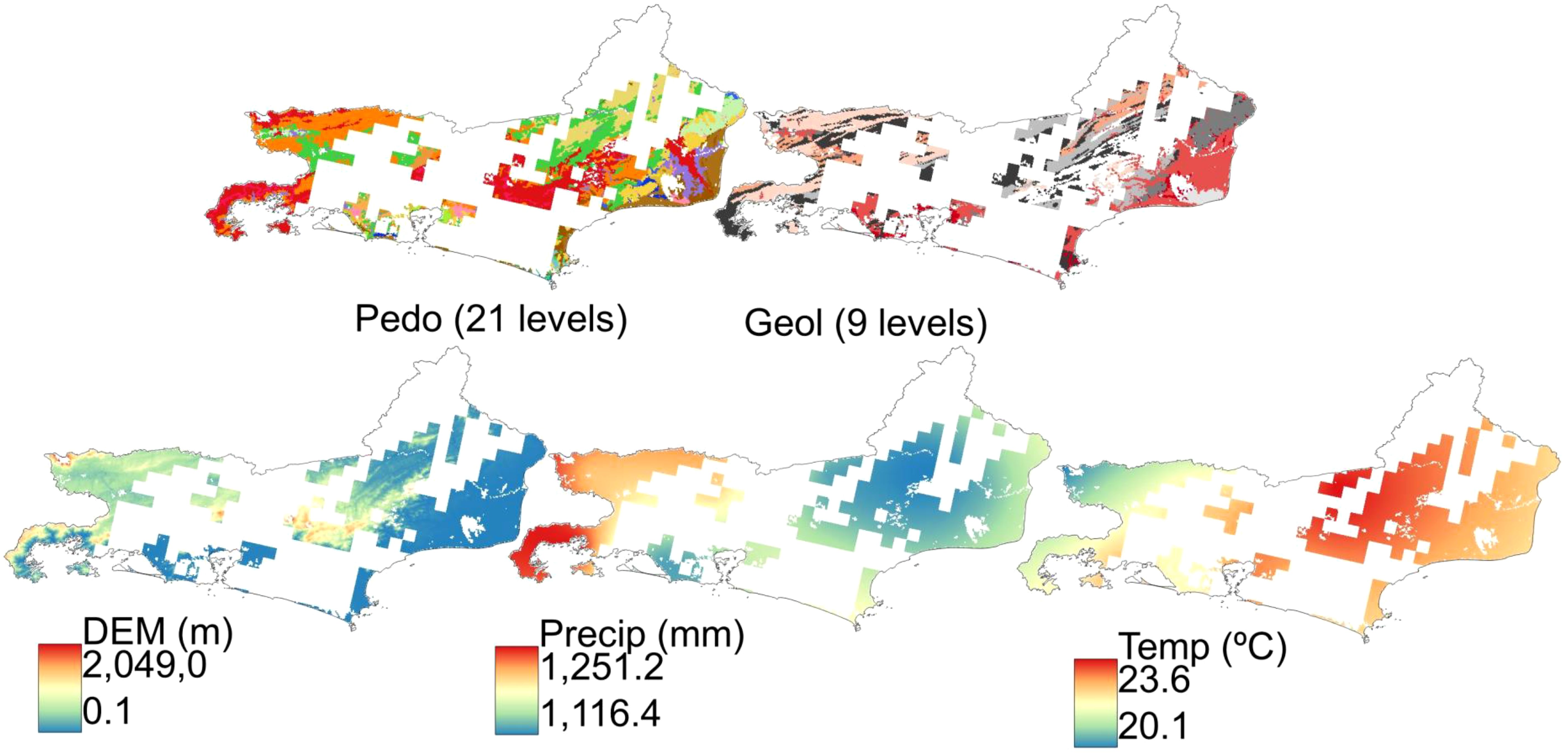
Figure 15. Covariables cropped for Rio de Janeiro’s reference area, with a block size of 10 and a target area of 50% delineated by the autoRA.

The temperature and precipitation gradients are driven by the state’s varied elevation and climatic patterns (49). Parent material, including crystalline rocks in the Serra do Mar and sedimentary deposits in the coastal plains, further drives the variability in soil mineralogy and texture, as highlighted in the geology map (50) (Figure 15, Geol). The pedology map (Figure 15, Pedo) underscores the diversity of soil types, from highly weathered Oxisols in upland regions to Quartzipsamments in the coastal plains, capturing the stark transitions driven by relief and parent material. Additionally, the elevation map reflects the role of topography in shaping soil formation, where steep slopes favor shallow soils like Entisols, while flatter areas support deeper, weathered soils (51, 52).

The frequency distributions of pixel values for the RA-masked covariates and the EPM in Rio de Janeiro are shown in Figure 16. It reveals that the pixels inside the RA chosen for Rio de Janeiro (RAM, target area 50% and block size 10) encapsulated the same variability in pixels in the whole extension of the Study Area (EPM). For pedology, the RAM represented all 21 soil classes, including dominant types such as Oxisols and Ultisols, as well as less prevalent ones like Entisols. This ensures that the RAM dataset encompasses the full range of soil variability, preserving critical transitions between highly weathered upland soils and poorly developed sandy soils in the coastal plains.

Figure 16

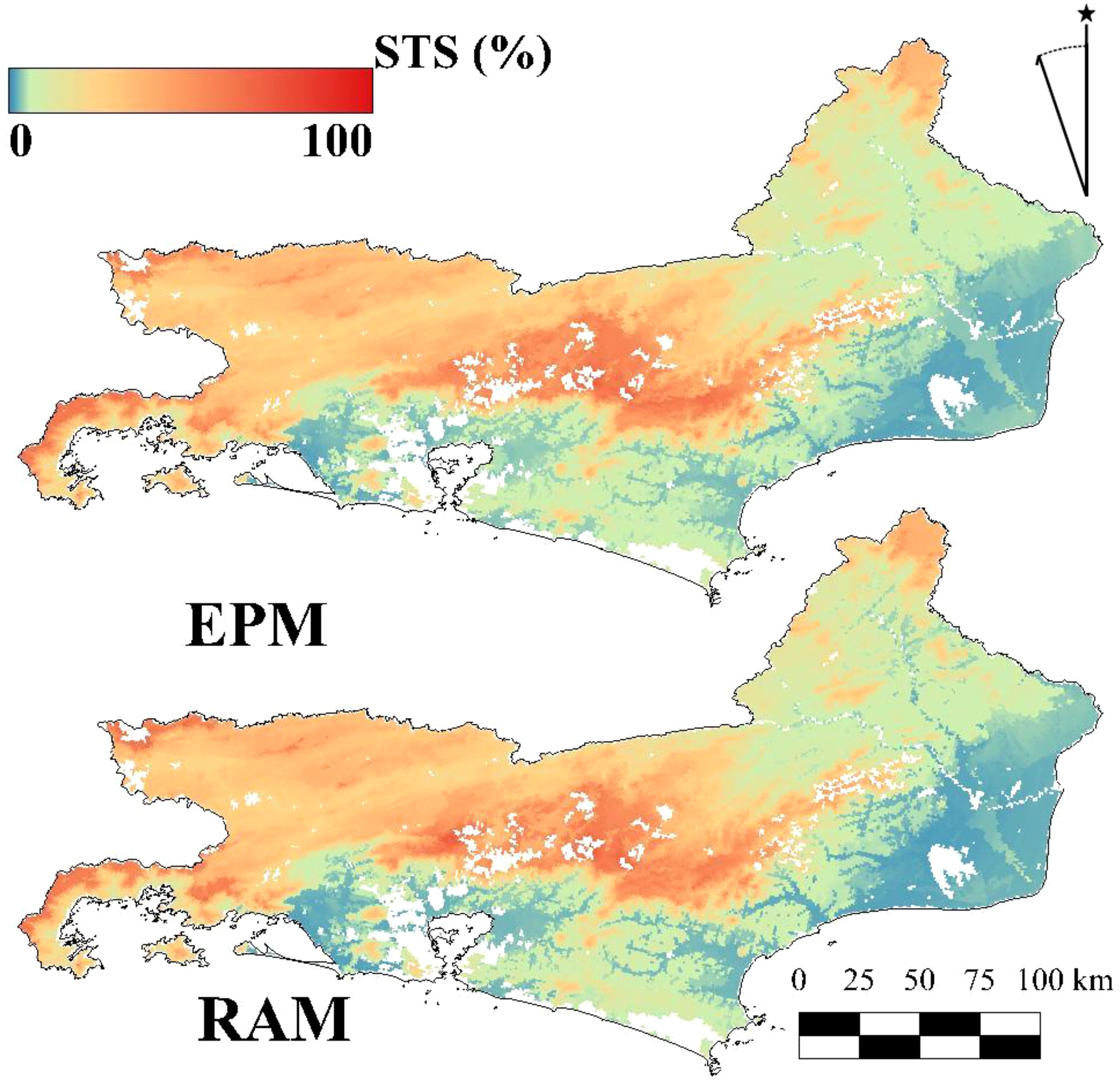
Figure 16. Comparison for the predicted Simulated Theoretical Surface (STS) maps via Exhaustive Prediction Model (EPM) using the whole area sampling strategy and Reference Area Model (RAM) using autoRA for Rio de Janeiro.

Similarly, the geology covariate, which includes nine lithological classes, is well-represented in RAM by capturing the central geological units, such as crystalline rocks and sedimentary deposits, strongly influencing soil mineralogy and texture across the landscape. The RAM effectively captures the full range of variability observed in the EPM for climatic variables, such as temperature and precipitation. Temperature gradients from 20°C to 24°C and precipitation values between 1,116 mm and 1,250 mm are consistently represented, ensuring that the climatic influences on soil formation, such as leaching and organic matter accumulation, are adequately accounted for (Figure 16).

The elevation covariate (Figure 16, DEM), which spans from sea level to 2,049 meters, is similarly preserved in RAM. The frequency distribution indicates a proportional representation of low-lying areas, mid-elevations, and higher terrains, reflecting the dynamic role of relief in shaping soil properties. Steep slopes associated with shallow, eroded soils (e.g., Entisols) and flatter regions where deep weathering occurs (e.g., Oxisols) are included in the RAM dataset, ensuring that topographically driven variability is maintained.

Figure 17 demonstrates that the RAM delineated by autoRA with a target area covering 50% of the total Study Area can effectively map the SPS for Rio de Janeiro. It produces results nearly identical to those of the EPM, significantly saving time and resources. Visual comparisons highlight the similarity between the two approaches, underscoring RAM’s potential for efficient and accurate environmental mapping and offering a cost-effective alternative to EPM without compromising quality.

Figure 17

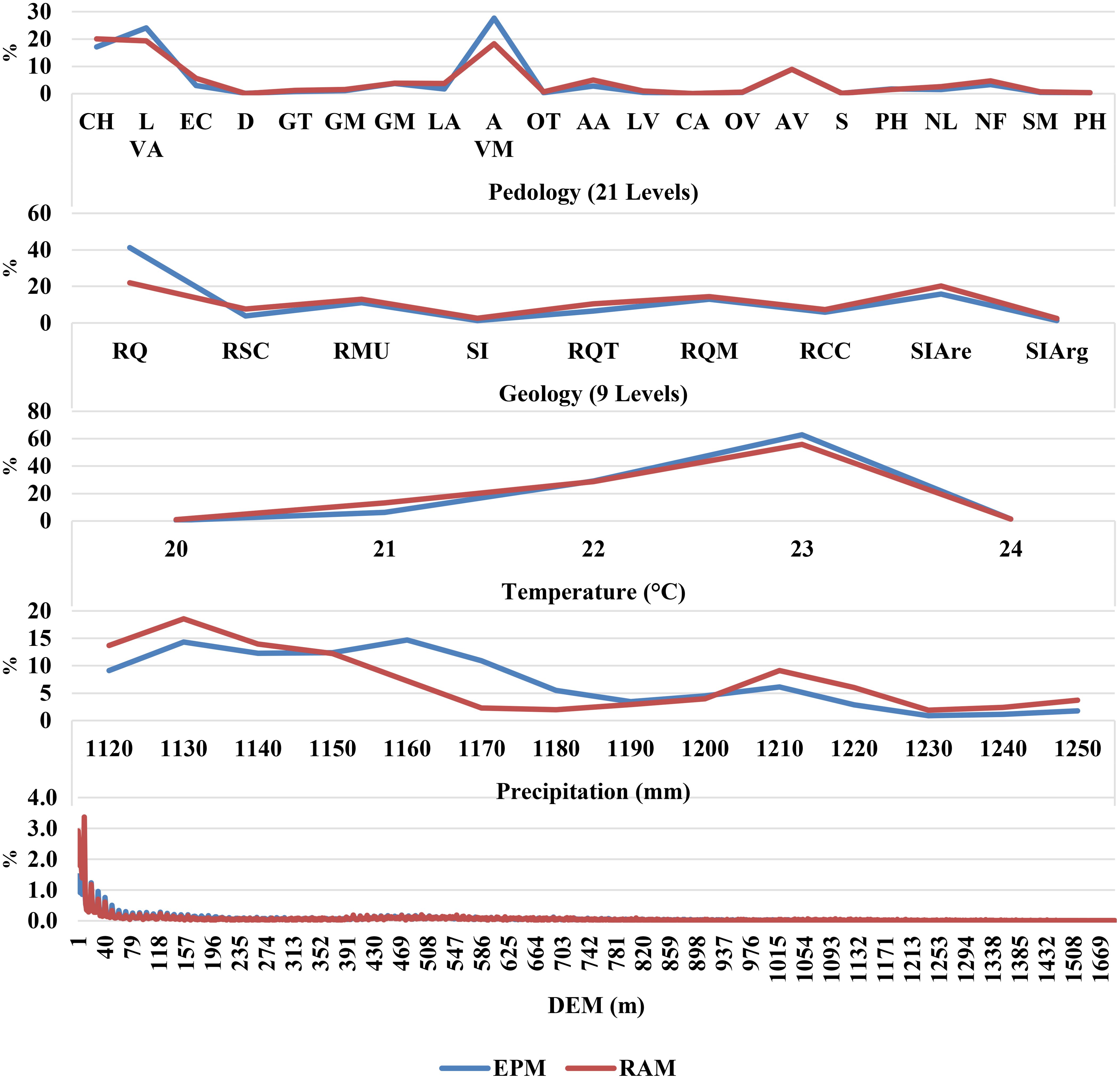
Figure 17. Frequency of pixel information for Exhaustive Prediction Model (EPM) and Reference Area Model (RAM). Pedology map: CH, Typic Dystrudept; LVA, Red-Yellow Oxisol; EC, Carbic Spodosol; D, Dunes; GT, Thionic Gleysol, e.g., Typic Sulfaquept; GM, Melanic Gleysol, GH, Haplic Gleysol, e.g., Typic Endoaquept; LA, Yellow Oxisol; AVM, Red-Yellow Ultisol; OT, Thionic Organosol, e.g., Typic Sulfosaprist; AA, Yellow Ultisol; LV, Red Oxisol; CA, Argiluvic Chernozem, e.g., Typic Haplustoll; OH, Haplic Organosol, e.g., Typic Haplosaprist; AV, Red Ultisol; S, Saline soils; PH, Hydromorphic Planosol, e.g., Typic Albaqualf; NL, Lithic Entisol; NF, Fluvent, SM, Mangrove soils; PH, Haplic Planosol, e.g., Typic Albaqualf. Geology map: RQ, Quartz-feldspathic rocks; RSC, Clastic sedimentary rocks; RMU, Mafic, and ultramafic rocks; SI, Unconsolidated sediments; RQT, Quartzose rocks; RQM, Micaeous quartz-feldspathic rocks; RCC, Carbonatic and calcium-silicate rocks; SIAre, Sandy unconsolidated sediments; SIArg, Clayey unconsolidated sediments.

3.4 Evaluating autoRA: contrasts and synergies with established sampling approaches in digital soil mapping

The autoRA represents a novel strategy within the broader field of DSM, which has seen numerous methodologies proposed to optimize sampling designs, balance cost efficiency, and maintain robust predictive performance. To better understand how autoRA aligns with or diverges from the current sampling approaches, this section contrasts autoRA’s methodology with four main lines of work: (i) conditioned Latin hypercube sampling (cLHS), (ii) Homosoils, (iii) sampling designs optimizing variance between population and sample sets (53), and (iv) divergence-based approaches for determining sample size (2, 54). Although each approach seeks to effectively capture environmental heterogeneity, it differs substantially in its theoretical underpinnings, implementation, and adaptability to varying soil-landscape contexts.

3.4.1 Contrasts with conditioned Latin hypercube sampling

Conditioned Latin hypercube sampling (cLHS) has long been recognized as a robust technique for generating a stratified random sample across relevant covariates (16). By projecting environmental variables into a multidimensional feature space, cLHS endeavors to sample each stratum equally, thereby ensuring coverage of the covariate distribution (55). However, cLHS presupposes a priori fixed number of samples, which can be problematic in large or heterogeneous regions. Once the number of samples is decided, cLHS does not inherently recalibrate or refine its sampling plan based on new information about soil variability (2). This limitation may lead to the oversampling of relatively uniform areas or failure to capture underrepresented yet pedologically significant zones if the initial stratification proves suboptimal.

In contrast, autoRA continuously gauges spatial heterogeneity via Gower’s Dissimilarity Index. By systematically delineating RAs and testing them against performance metrics such as R², RMSE, and Bias, combining them with a sensitivity analysis of different target areas and block sizes, autoRA iteratively refines its sampling scope before the fieldwork itself. Hence, while cLHS frontloads the sampling design process, autoRA incorporates feedback loops that dynamically adjust reference-area boundaries and sampling densities. This responsive mechanism is particularly beneficial in regions where heterogeneity is high, there is difficult to access the sampling locations, or is not evenly distributed, such as mountainous areas or wetlands (54). Additionally, cLHS and autoRA are not mutually exclusive; in principle, autoRA’s final delineated RAM could incorporate a cLHS-type scheme for spatial allocation of actual sample sites, if desired. Nonetheless, autoRA’s core advantage is its real-time adaptability, which mitigates reliance on static sampling targets and helps manage logistical constraints (e.g., limited field operability and safety concerns).

3.4.2 Contrasts with homosoils

Homosoils, as presented by Nenkam et al. (56, 57), similarly uses Gower’s dissimilarity index to cluster pedologically similar areas and direct sampling toward zones of maximum dissimilarity. In doing so, Homosoils aims to avoid oversampling landscapes that exhibit relative uniformity while focusing resources on capturing critical variability. This conceptual foundation parallels autoRA’s objective of capturing diverse soil formation factors by prioritizing environmental heterogeneity.

However, Homosoils typically pre-specifies a sampling density or cluster count without explicitly integrating metrics of predictive accuracy – such as R², RMSE, or Bias – into its final selection process. In contrast, autoRA explicitly uses a Random Forest model on a simulated theoretical surface (STS), running multiple sensitivity analyses (block sizes, target areas) and computing an Euclidean Distance (ED) aggregate of prediction metrics. AutoRA chooses the “optimal” RA arrangement only after running these iterations. Consequently, autoRA identifies the region(s) of highest dissimilarity and verifies that sampling these regions demonstrably leads to predictive gains, thereby establishing a direct link between sampling design and model performance. This systematic feedback mechanism differentiates autoRA from Homosoils, offering a more robust criterion for deciding the optimal coverage while leveraging the core principle that areas of high Gower’s Dissimilarity Index merit more careful sampling.

3.4.3 Contrasts with variance-based sampling designs

Stumpf et al. (53) addressed the challenge of defining an optimal sample size by comparing the variance of the covariate population to that of the sample set. Their methodology incrementally increased sample size, using box plots and density plots of relevant covariates to identify a threshold at which additional sampling yielded diminishing returns in capturing population variance (58). This approach offers a transparent and intuitive means of sampling: once the sample’s variance profile sufficiently approximates that of the population, the design is considered “good enough.”

While straightforward and conceptually appealing, variance-based sampling primarily hinges on matching statistical moments of the covariate distribution, which may not always capture deeper or more complex pedological relationships (2). For instance, variance equivalence does not necessarily account for underlying spatial patterns or the combined effect of covariates, which might be crucial in regions where soil properties are influenced by intricate interactions of climate, relief, and parent material (1). In contrast, autoRA’s reliance on Gower’s Dissimilarity Index (59) and comprehensive metrics (R², RMSE, Bias) ensures that the final RA delineation does more than match a univariate or bivariate variance profile; it also demonstrates robust predictive fidelity for the soil attributes of interest by offering a derivate Simulated Theoretical Surface that is mapped, and the accuracy is evaluated before the fieldwork starts. Another distinguishing factor lies in autoRA’s reliance on sensitivity analysis across multiple parameter settings rather than a single stepwise approach to sample size increments. This approach simultaneously refines both the size and shape of the RA, reducing the risk of focusing solely on variable variance while missing other dimensions of soil heterogeneity (53).

3.4.4 Contrasts with divergence-based approaches for determining sample size

Divergence-based approaches have gained attention for their potential in determining optimal sample size by comparing differences in probability distributions. Malone et al. (2) employed the Kullback-Leibler Divergence (DKL) statistic to evaluate how closely a sample’s empirical distribution function (EDF) approximates that of the larger population. By finding the point of “diminishing returns” in the DKL curve, one can infer an optimal sample size that balances coverage with practical resource limitations.

Building on this concept, Saurette et al. (54) introduced the Jensen-Shannon Divergence (DJS) and the related Jensen-Shannon Distance (Dist_JS) as more robust, symmetric metrics for appraising how well a given sample distribution matches the population distribution. These divergence metrics require binning the data into histograms or probability distribution functions (PDFs) and comparing how closely the sample’s PDF aligns with the entire domain. In principle, DKL, DJS, or Dist_JS can reveal the “breakpoint” beyond which additional sampling yields marginal improvements in distribution matching. Divergence-based methods thus offer a mathematically elegant solution to determining an “optimal” sample size that captures the principal features of the covariate space.

Yet, like variance-based techniques, divergence-based approaches often treat each covariate or histogram dimension independently (2, 54). While they are more holistic than a single variance measure, they still may not fully capture spatial autocorrelation patterns or complex covariate interactions that strongly influence soil genesis and variability. In contrast, autoRA applies a Random Forest framework to evaluate how well the delineated RAM can predict an STS, encapsulating multiple covariates simultaneously in a respective smaller region. The final selection of target area and block size is thus informed by direct modeling performance, not solely distribution matching. Consequently, autoRA can integrate the strengths of divergence-based analyses – identifying representativeness thresholds – while going further by ensuring that this representativeness translates into tangible predictive accuracy. Indeed, future versions of autoRA could incorporate DJS or Dist_JS as complementary indices alongside Gower’s dissimilarity, providing an even more refined synergy between statistical distribution matching and predictive modeling.

3.4.5 Synthesis and outlook

Taken together, these comparisons underscore the distinctiveness and adaptability of autoRA. Conditioned Latin hypercube sampling (cLHS) ensures an even distribution of samples across covariate space but does not dynamically adjust to local heterogeneity or feedback from model performance. Homosoils likewise leverage Gower’s Dissimilarity Index to detect uniform vs. highly variable areas but does not explicitly integrate predictive metrics into the sampling density decision neither shows the smaller area capable to be sampled and represent the interest study area. Variance-based sample size selection (53) provides a straightforward mechanism for aligning sample distributions with population variance but can overlook complex multidimensional relationships and also does not consider the hypothesis of searching and minimizing the investigation area based on the Reference Area approach. Divergence-based approaches (2, 54) offer mathematically rigorous methods for defining optimal sample sizes by comparing distribution functions, yet they may underserve spatial context or joint covariate interactions and also does not consider the hypothesis of minimizing the sampling area to produce a model for extrapolation.

By contrast, autoRA weaves together the strengths of spatial dissimilarity assessment (via Gower’s Dissimilarity Index), iterative modeling (via Random Forest) and Simulation Theoretical Surface, and sensitivity analyses (varying target areas and block sizes) into a single workflow. This ensures that representativeness, cost-effectiveness, and predictive reliability are simultaneously prioritized. Moreover, autoRA’s capacity to include other divergence metrics or sampling heuristics signals a pathway for future enhancements, making it a flexible platform for integrating new advances in DSM. As a result, autoRA stands out not merely as another sampling design tool but as a dynamic framework that combines data-driven delineation of RAs with tangible model performance evaluation – critical for robust and scalable soil mapping in the face of limited ground-truth data.

4 Conclusions

The autoRA algorithm demonstrated a robust, data-driven approach for delineating RAs representing critical soil-forming factors, enabling more efficient and accurate digital soil mapping workflows. By employing Gower’s Dissimilarity Index to capture environmental heterogeneity, autoRA systematically identified configurations of target area size and spatial resolution (block size) that balanced predictive performance and cost. The optimal RAM with a 50% target area and a block size of 10, autoRA achieved ED values (0.15 in Rio de Janeiro and 0.38 in Florida) closely approximating the benchmarks obtained using exhaustive sampling (0.17 and 0.35, respectively) while reducing total costs by approximately US$110,000. This translates to cost reductions of about 61% in Rio de Janeiro and 63% in Florida compared to the traditional reference approach.

Beyond this optimal setting, several other combinations offered even more significant cost savings, albeit with marginal trade-offs in accuracy. For instance, at a 30% target area and a 10x10 km² block size, the model in Rio de Janeiro produced an ED of around 0.33. In contrast, for the same target area value, the resolution of 5x5 km² for Florida produced an ED close to 0.40 – slightly higher than the optimal scenario – yet costs were cut by about 80%. Similarly, other parameter settings at smaller target areas (e.g., 20%) and moderate block sizes (e.g., 10 or 20 pixels) delivered substantial cost-efficiency while maintaining acceptable ED values. These findings highlight autoRA’s versatility, allowing practitioners to tailor the balance between accuracy and cost according to specific project constraints, logistical limitations, and data requirements.

By reducing subjective expert input and introducing a reproducible, quantitative framework for RA delineation, autoRA enables more strategic investments in soil sampling. Its capacity to preserve predictive quality while substantially lowering expenses makes it a valuable tool, particularly in regions where field sampling is logistically challenging or financially constrained. Ultimately, this approach strengthens DSM workflows, fosters broader coverage in data-scarce landscapes, and supports more informed decision-making in soil resource management.

Data availability statement

The raw data supporting the conclusions of this article will be made available by the authors, without undue reservation.

Author contributions

HR: Data curation, Formal Analysis, Investigation, Methodology, Software, Validation, Writing – original draft, Writing – review & editing. MC: Conceptualization, Data curation, Formal Analysis, Funding acquisition, Investigation, Methodology, Project administration, Resources, Supervision, Validation, Visualization, Writing – original draft, Writing – review & editing. GV: Conceptualization, Data curation, Formal Analysis, Investigation, Methodology, Supervision, Visualization, Writing – original draft, Writing – review & editing. SG: Conceptualization, Data curation, Formal Analysis, Funding acquisition, Investigation, Methodology, Project administration, Resources, Software, Supervision, Validation, Visualization, Writing – original draft, Writing – review & editing. EB: Methodology, Supervision, Validation, Visualization, Writing – review & editing.

Funding

The author(s) declare that financial support was received for the research and/or publication of this article. This research was funded by Coordenação de Aperfeiçoamento de Pessoal de Nível Superior (CAPES), with a Ph.D. scholarship for the author under the number 161334/2021-0.

Conflict of interest

The authors declare that the research was conducted in the absence of any commercial or financial relationships that could be construed as a potential conflict of interest.

The author(s) declared that they were an editorial board member of Frontiers, at the time of submission. This had no impact on the peer review process and the final decision.

Generative AI statement

The author(s) declare that Generative AI was used in the creation of this manuscript. Grammarly.

Publisher’s note

All claims expressed in this article are solely those of the authors and do not necessarily represent those of their affiliated organizations, or those of the publisher, the editors and the reviewers. Any product that may be evaluated in this article, or claim that may be made by its manufacturer, is not guaranteed or endorsed by the publisher.

Supplementary material

The Supplementary Material for this article can be found online at: https://www.frontiersin.org/articles/10.3389/fsoil.2025.1557566/full#supplementary-material

References

1. McBratney AB, Mendonça Santos ML, Minasny B. On digital soil mapping. Geoderma. (2003) 117:3–52. doi: 10.1016/S0016-7061(03)00223-4

Crossref Full Text | Google Scholar

2. Malone BP, Minasny B, Brungard C. Some methods to improve the utility of conditioned Latin hypercube sampling. PeerJ. (2019) 7:e6451. doi: 10.7717/peerj.6451

PubMed Abstract | Crossref Full Text | Google Scholar

3. Khaledian Y, Miller BA. Selecting appropriate machine learning methods for digital soil mapping. Appl Math Modelling. (2020) 81:401–18. doi: 10.1016/j.apm.2019.12.016

Crossref Full Text | Google Scholar

4. Chen L, Wang W, Wang C, Yan X, Zhang Y, Shen Z. From field soil sampling to watershed model: Upscaling by integrating information entropy and interpolation method. J Environ Management. (2024) 360:121119. doi: 10.1016/j.jenvman.2024.121119

PubMed Abstract | Crossref Full Text | Google Scholar

5. Malone BP, Styc Q, Minasny B, McBratney AB. Digital soil mapping of soil carbon at the farm scale: A spatial downscaling approach in consideration of measured and uncertain data. Geoderma. (2017) 290:91–9. doi: 10.1016/j.geoderma.2016.12.008

Crossref Full Text | Google Scholar

6. Hengl T, Jesus JM, MacMillan RA, Batjes NH, Heuvelink GBM, Ribeiro E, et al. SoilGrids1km — Global soil information based on automated mapping. PloS One. (2014) 9:e105992. doi: 10.1371/journal.pone.0105992

PubMed Abstract | Crossref Full Text | Google Scholar

7. Poggio L, de Sousa LM, Batjes NH, Heuvelink GBM, Kempen B, Ribeiro E, et al. SoilGrids 2.0: producing soil information for the globe with quantified spatial uncertainty. SOIL. (2021) 7:217–40. doi: 10.5194/soil-7-217-2021

Crossref Full Text | Google Scholar

8. Favrot JC. “Pour une approche raisoneé du drainage agricole en France. La Méthode Des Secteurs de Référence.” C.R. Académie d’Agriculture de France, Paris, France (1981) 67(8):716–23.

Google Scholar

9. Lagacherie P, Robbez-Masson JM, Nguyen-The N, Barthès JP. Mapping of reference area representativity using a mathematical soilscape distance. Geoderma. (2001) 101:105–18. doi: 10.1016/S0016-7061(00)00101-4

Crossref Full Text | Google Scholar

10. Lagacherie P, Legros JP, Burrough PA. A soil survey procedure using the knowledge of soil pattern established on a previously mapped reference area. Geoderma. (1995) 65:283–301. doi: 10.1016/0016-7061(94)00040-H

Crossref Full Text | Google Scholar

11. Ferreira AC, de S, Ceddia MB, Costa EM, Pinheiro ÉFM, Nascimento MM, et al. Use of airborne radar images and machine learning algorithms to map soil clay, silt, and sand contents in remote areas under the amazon rainforest. Remote Sensing. (2022) 14:5711. doi: 10.3390/rs14225711

Crossref Full Text | Google Scholar

12. Arruda GP, Demattê JAM, Chagas CdaS, Fiorio PR, Souza AB, Fongaro CT. Digital soil mapping using reference area and artificial neural networks. Scientia Agricola. (2016) 73:266–73. doi: 10.1590/0103-9016-2015-0131

Crossref Full Text | Google Scholar

13. Ferreira ACS, Pinheiro ÉFM, Costa EM, Ceddia MB. Predicting soil carbon stock in remote areas of the Central Amazon region using machine learning techniques. Geoderma Regional. (2023) 32:e00614. doi: 10.1016/j.geodrs.2023.e00614

Crossref Full Text | Google Scholar

14. Jean-Marc Robbez-Masson. Reconnaissance et délimitation de motifs d’organisation spatiale. Application à la cartographie des pédopaysages. Thesis. Montepellier: École Nationale Supérieure Agronomique de Montpellier (1994).

Google Scholar

15. ten Caten A, Dalmolin RSD, Pedron F, Santos M. Extrapolação das relações solo-paisagem a partir de uma área de referência. Ciec Rural. (2011) 41:812–6. doi: 10.1590/S0103-84782011000500012

Crossref Full Text | Google Scholar

16. Minasny B, McBratney AB. A conditioned Latin hypercube method for sampling in the presence of ancillary information. Comput Geosciences. (2006) 32:1378–88. doi: 10.1016/j.cageo.2005.12.009

Crossref Full Text | Google Scholar

17. Moura DMBD, Oliveira IJD, Nascimento DTF, Sousa FAD. Refinamento do mapa de solos da alta bacia hidrográfica do Ribeirão Santa Marta, estado de Goiás, Brasil. Caderno Geografia. (2020) 30:865. doi: 10.5752/P.2318-2962.2020v30n62p865

Crossref Full Text | Google Scholar

18. Canavesi V, Segoni S, Rosi A, Ting X, Nery T, Catani F, et al. Different approaches to use morphometric attributes in landslide susceptibility mapping based on meso-scale spatial units: A case study in rio de janeiro (Brazil). Remote Sensing. (2020) 12:1826. doi: 10.3390/rs12111826

Crossref Full Text | Google Scholar

19. Filippini-Alba JM, Flores C-A, Bernardi AC. Pedology in precision agriculture from a Brazilian context. Rev Ciências Agrícolas. (2023) 40:e3216. doi: 10.22267/rcia.20234003.216

Crossref Full Text | Google Scholar

20. Vasconcelos BNF, Bravo JVM, Cunha JEF, Fernandes-Filho EI. Mapping the soil frontiers with legacy soil data: an approach for covering the lack of updated reference maps of minas gerais, Brazil. Anuário do Instituto Geociências. (2023) 46:1–11. doi: 10.11137/1982-3908_2023_46_49327

Crossref Full Text | Google Scholar

21. Nauman TW, Kienast-Brown S, Roecker SM, Brungard C, White D, Philippe J, et al. Soil landscapes of the United States (SOLUS): Developing predictive soil property maps of the conterminous United States using hybrid training sets. Soil Sci Soc America J. (2024) 88:2046–65. doi: 10.1002/saj2.20769

Crossref Full Text | Google Scholar

22. Gower JC. A general coefficient of similarity and some of its properties. Biometrics. (1971) 27:857–71. doi: 10.2307/2528823

Crossref Full Text | Google Scholar

23. Gauld DB. Topological properties of manifolds. Am Math Monthly. (1974) 81:633–6. doi: 10.1080/00029890.1974.11993635

Crossref Full Text | Google Scholar

24. O'Searcóid M. Metric Spaces. Springer Undergraduate Mathematics Series. London: Springer London Springer e-books, 2007.

Google Scholar

25. Ferry S, Weinberger S. Quantitative algebraic topology and Lipschitz homotopy. Proc Natl Acad Sci. (2013) 110:19246–50. doi: 10.1073/pnas.1208041110

Crossref Full Text | Google Scholar

26. Falconer KJ, Marsh DT. On the Lipschitz equivalence of Cantor sets. Mathematika. (1992) 39:223–33. doi: 10.1112/S0025579300014959

Crossref Full Text | Google Scholar

27. Sellards EH. Geology of florida. J Geology. (1919) 27:286–302. doi: 10.1086/622662

Crossref Full Text | Google Scholar

28. LaPierre GDJ, Irizarry NDM, Andreu MG. Florida soil series and natural community associations: FOR384 FR455, 5 2022. EDIS. (2022) 2022:(3). doi: 10.32473/edis-fr455-2022

Crossref Full Text | Google Scholar

29. Watts FC, Collins ME. Formation of the soils in florida. In: Madison WI, editor. Soils of florida, 1st. American Society of Agronomy and Soil Science Society of America, USA (2008). p. 1–28. doi: 10.2136/2008.soilsofflorida.c1

Crossref Full Text | Google Scholar

30. Heilbron M, do Silva LGE, De Almeida JCH, Tupinambá M, Peixoto C, de Valeriano CM, et al. Proterozoic to Ordovician geology and tectonic evolution of Rio de Janeiro State, SE-Brazil: insights on the central Ribeira Orogen from the new 1:400,000 scale geologic map. Braz J Geology. (2020) 50:e20190099. doi: 10.1590/2317-4889202020190099

Crossref Full Text | Google Scholar

31. Junior PRPR, Nascimento FRD. Environment, geology-geomorphology and water availability in the Guandu river basin/Rio de Janeiro. William Morris Davis - Rev Geomorfologia. (2022) 3:1–20. doi: 10.48025/ISSN2675-6900.v3n1.2022.147

Crossref Full Text | Google Scholar

32. IBGE. “Mapeamento de Recurso Naturais do Brasil Escala 1:250.000” in Documentação Técnica Geral. Rio de Janeiro, Brazil: Diretoria de Geociências, Coordenação de Recursos Naturais e Estudos Ambientais (2018).

Google Scholar

33. Gelsleichter YA, Costa EM, Anjos LHCD, Marcondes RAT. Enhancing Soil Mapping with Hyperspectral Subsurface Images generated from soil lab Vis-SWIR spectra tested in southern Brazil. Geoderma Regional. (2023) 33:e00641. doi: 10.1016/j.geodrs.2023.e00641

Crossref Full Text | Google Scholar

34. Pereira MG, Anjos LHC. Formas extraíveis de ferro em solos do estado do Rio de Janeiro. Rev Bras Ciec do Solo. (1999) 23:371–82. doi: 10.1590/S0100-06831999000200020

Crossref Full Text | Google Scholar

35. Pereira MG, Anjos LHCD, Neto ECDS, Junior CRP. Solos do Rio de Janeiro - Gênese, classificação e limitações ao uso agrícola. 1st. Paraná, Brazil: Atena Editora (2023). doi: 10.22533/at.ed.273232510

Crossref Full Text | Google Scholar

36. Jenny H. Factors of soil formation: a system of quantitative pedology. In: Dover books on earth sciences. Foreword by ronald amundson. Dover Publications, New York, USA (1994). New York : McGraw-Hill, 1941. With new foreword. Includes bibliographical references and index.

Google Scholar

37. Soil Survey Staff, Natural Resources Conservation Service. Web soil survey (2016). Available online at: http://websoilsurvey.nrcs.usda.gov (Accessed 23 December 2024).

Google Scholar

38. Horton JD. The State Geologic Map Compilation (SGMC) geodatabase of the conterminous United States (ver. 1.1, August 2017): U.S. Geological Survey data release. (2017). doi: 10.5066/F7WH2N65

Crossref Full Text | Google Scholar

39. PRISM Climate Group. Oregon State University. (2012) https://prism.oregonstate.edu (Accessed Septemmber 17, 2024).

Google Scholar

40. Fick SE, Hijmans RJ. WorldClim 2: new 1-km spatial resolution climate surfaces for global land areas. Int J Climatology. (2017) 37:4302–15. doi: 10.1002/joc.5086

Crossref Full Text | Google Scholar

41. Meyer H, Pebesma E. Predicting into unknown space? Estimating the area of applicability of spatial prediction models. Methods Ecol Evolution. (2021) 12:1620–33. doi: 10.1111/2041-210X.13650

Crossref Full Text | Google Scholar

42. Liaw A, Wiener M. Classification and Regression by randomForest. In: R news (Austria: The R Foundation), vol. 2. (2002). p. 18–22. Available at: https://CRAN.R-project.org/doc/Rnews/ (Accessed November 11, 2024).

Google Scholar

43. R Core Team. R: A language and environment for statistical computing (2024). Available online at: https://www.R-project.org/ (Accessed November 11, 2024).

Google Scholar

44. Clingensmith CM, Grunwald S. Predicting soil properties and interpreting vis-NIR models from across continental United States. Sensors. (2022) 22:3187. doi: 10.3390/s22093187

PubMed Abstract | Crossref Full Text | Google Scholar

45. United States Census Bureau. 2022 TIGER/Line Shapefiles (machine readable data files). (2019) U.S. Department of Commerce. https://www.census.gov/cgi-bin/geo/shapefiles/index.php (Accessed 21 November 2024).

Google Scholar

46. Costa EM, Rodrigues HM, Ferreira Souza AC, Ceddia MB, Fernandes Corrêa DA. “Using Legacy Soil Data to Plan New Data Collection: Study Case of Rio de Janeiro State: Brazil.” In Pedometrics in Brazil. Junior Carvalho W, Pinheiro Koenow HS, Ceddia MB, Valladares GS. Cham: Springer Nature Switzerland (2024), 101–13. doi: 10.1007/978-3-031-64579-2_8

Crossref Full Text | Google Scholar

47. Brus DJ. Statistical sampling approaches for soil monitoring. Eur J Soil Science. (2014) 65:779–91. doi: 10.1111/ejss.12176

Crossref Full Text | Google Scholar

48. Heil K, Schmidhalter U. The application of EM38: determination of soil parameters, selection of soil sampling points and use in agriculture and archaeology. Sensors. (2017) 17:2540. doi: 10.3390/s17112540

PubMed Abstract | Crossref Full Text | Google Scholar

49. Neiva H, Da Silva M, Cardoso C. Analysis of climate behavior and land use in the city of rio de janeiro, RJ, Brazil. Climate. (2017) 5:52. doi: 10.3390/cli5030052

Crossref Full Text | Google Scholar

50. Pinheiro Junior CR, Pereira MG, Azevedo AC, de Van Huyssteen C, dos Anjos LHC, Fontana A, et al. Genesis and classification of carbonate soils in the State of Rio de Janeiro, Brazil. J South Am Earth Sci. (2021) 108:103183. doi: 10.1016/j.jsames.2021.103183

Crossref Full Text | Google Scholar

51. Gonçalves RVS, Cardoso JCF, Oliveira PE, Raymundo D, de Oliveira DC. The role of topography, climate, soil and the surrounding matrix in the distribution of Veredas wetlands in central Brazil. Wetlands Ecol Management. (2022) 30:1261–79. doi: 10.1007/s11273-022-09895-z

Crossref Full Text | Google Scholar

52. Fontana A, Chagas C, da S, Donagemma GK, Menezes AR, Calderano B. Soils developed on geomorphic surfaces in the mountain region of the state of rio de janeiro. Rev Bras Ciênc. Solo. (2017) 41:1–17. doi: 10.1590/18069657rbcs20160574

Crossref Full Text | Google Scholar

53. Stumpf F, Schmidt K, Behrens T, Schönbrodt-Stitt S, Buzzo G, Dumperth C, et al. Incorporating limited field operability and legacy soil samples in a hypercube sampling design for digital soil mapping. J Plant Nutr Soil Science. (2016) 179:499–509. doi: 10.1002/jpln.201500313

Crossref Full Text | Google Scholar

54. Saurette DD, Heck RJ, Gillespie AW, Berg AA, Biswas A. Divergence metrics for determining optimal training sample size in digital soil mapping. Geoderma. (2023) 436:116553. doi: 10.1016/j.geoderma.2023.116553

Crossref Full Text | Google Scholar

55. Sena NC, Veloso GV, Lopes AO, Francelino MR, Fernandes-Filho EI, Senra EO, et al. Soil sampling strategy in areas of difficult access using the cLHS method. Geoderma Regional. ((2021)) 24:e00354. doi: 10.1016/j.geodrs.2020.e00354

Crossref Full Text | Google Scholar

56. Nenkam AM, Wadoux AMJ, Minasny B, McBratney AB, Traore PCS, Falconnier GN, et al. Using homosoils for quantitative extrapolation of soil mapping models. Eur J Soil Science. (2022) 73:e13285. doi: 10.1111/ejss.13285

Crossref Full Text | Google Scholar

57. Nenkam AM, Wadoux AMJ-C, Minasny B, McBratney AB, Traore PCS, Whitbread AM. Using homosoils to enrich sparse soil data infrastructure: An example from Mali. CATENA. (2023) 223:106862. doi: 10.1016/j.catena.2022.106862

Crossref Full Text | Google Scholar

58. Adams RA, Fournier JJF. 4 - the sobolev imbedding theorem. In: Pure and applied mathematics. Sobolev spaces. Amsterdam, The Netherlands: Elsevier (2003). p. 79–134. doi: 10.1016/S0079-8169(03)80006-5

Crossref Full Text | Google Scholar

59. de Carvalho Junior W, Saraiva Koenow Pinheiro H, Bacis Ceddia M, Souza Valladares G. Pedometrics in Brazil. Cham, Switzerland: Springer (2024).

Google Scholar