Groundwater fluoride prediction modeling using physicochemical parameters in Punjab, India: a machine-learning approach

Introduction: Rising fluoride levels in groundwater resources have become a worldwide concern, presenting a significant challenge to the safe utilization of water resources and posing potential risks to human well-being. Elevated fluoride and its vast spatial variability have been documented across different districts of Punjab, India, and it is, therefore, imperative to predict the fluoride levels for efficient groundwater resources planning and management.

Methods: In this study, five different models, Support Vector Machine (SVM), Random Forest (RF), Extreme Gradient Boosting (Xgboost), Extreme Learning Machine (ELM), and Multilayer Perceptron (MLP), are proposed to predict groundwater fluoride using the physicochemical parameters and sampling depth as predictor variables. The performance of these five models was evaluated using the coefficient of determination (R²), mean absolute error (MAE), and root mean square error (RMSE).

Results and discussion: ELM outperformed the remaining four models, thus exhibiting a strong predictive power. The R², MAE, and RMSE values for ELM at the training and testing stages were 0.85, 0.46, 0.36 and, 0.95, 0.31, and 0.33, respectively, while other models yielded inferior results. Based on the relative importance scores, total dissolved solids (TDS), electrical conductivity (EC), sodium (Na⁺), chloride (Cl⁻), and calcium (Ca²⁺) contributed significantly to model performance. High variability in the target (fluoride) and predictor variables might have led to the poor performance of the models, implying the need for better data pre-processing techniques to improve data quality. Although ELM showed satisfactory results, it can be considered a promising model for predicting groundwater quality.

1 Introduction

Consumption of groundwater with fluoride (F⁻) levels between 0.5–1.5 mg/L is essential for proper bone and tooth development. However, concentrations exceeding the recommended safe limit of 1.5 mg/L (1) can cause dental fluorosis (1.5–4.0 mg/L), skeletal fluorosis (4.0–10.0 mg/L), and several other disorders, including hypertension, renal failure, and cancer (> 10 mg/L) (2, 3). Reportedly, elevated F⁻ levels have already affected over 200 million people in 29 nations, including India (4). In India, F⁻ prevalence has been identified in 20 out of 29 states with 66 million inhabitants, including 6 million children, under the grasp of fluorosis (5, 6), with the numbers still expected to rise (7). Fluoride-bearing minerals, like fluorite, amphibole, mica, apatite, and biotite associated with host rocks like granite, mica, gneisses, etc., are the primary natural sources. Groundwater chemical conditions such as elevated alkalinity, reduced calcium levels, and sodium bicarbonate water type favor dissolution and desorption of metal oxides, causing F⁻ enrichment. Additionally, arid and semi-arid climatic zones have also reported increased F⁻ concentrations (8, 9) due to enhanced cation exchange capacity, dissolution from F⁻-bearing minerals and longer groundwater residence times, thereby increasing the interaction between the rock-water interface (10, 11). Besides the natural factors, anthropogenic activities, including phosphate fertilizer application, sewage and sludge dumping, mining, coal combustion, and excess groundwater extraction, also contribute to high F⁻ levels (11, 12).

Innumerable studies across Punjab have provided an overall picture of the state’s groundwater contamination problem. Fluoride concentrations have been reported in all the districts, particularly in the shallow aquifers, with more pronounced levels in the south and southwestern districts. For instance, F⁻ concentration in this region ranged from 0.1–17.5 mg/L in Bathinda, 0.34–8.24 mg/L in Fazilka (13), 0.15–11.6 mg/L in Mansa (14), and 1.5–9.2 mg/L in Patiala (15). Thus, this region has emerged as a hotspot of F⁻-contaminated groundwater (16, 17). The abundance of F⁻-bearing minerals, along with agricultural activities and industrial operations in this region, further enhance the contaminant levels in the groundwater system. The region’s climate, surface, and sub-surface conditions are conducive to dissolving, mobilizing, and enriching this contaminant in the aquifers. Punjab experiences meagre precipitation, high temperatures, and high evaporation rates linked to high total dissolved solids (TDS)/salinity, particularly in shallow aquifers. The aquifers are oxic and alkaline due to high bicarbonate concentrations. Additionally, the nitrate levels are prominent in shallow waters, probably due to agricultural runoff (17). All of these hydrochemical factors have a direct influence on F⁻ concentrations and, therefore, tend to intensify the contamination problem in this region. Hence, it is imperative to develop methodologies by integrating the in-situ measured variables from field surveys with other advanced and efficient techniques to strategize sustainable groundwater management plans and establish robust monitoring systems (18). Field-based groundwater monitoring is labor-intensive and expensive (19), in addition to the lab-based analytical procedures, which are tedious, complicated, and add a cost burden (20). In this context, various numerical and physical models, along with geospatial modeling, are often applied to comprehend the groundwater contamination process and the contributing factors (21, 22). However, these methods require huge datasets and an adequate hydrogeochemical understanding, which are mostly lacking in underdeveloped regions, leading to poor model performance (18, 23). Furthermore, the difficulty in interpreting the outputs of classical models and poor user-friendliness widen the gap between model creators and users. To bridge this gap, state-of-the-art machine-learning (ML) techniques are now being widely used to predict groundwater contamination.

Machine-learning models have been adopted extensively in the past several years to forecast a variety of contaminants in the groundwater due to their strong algorithms, flexible constraints, and reliable and accurate prediction performance (24). These techniques can also handle the non-linear relationships between the input and target variables efficiently, proving to be more robust than the conventional methods (25). Random Forest (RF) classification algorithm is widely used to forecast groundwater-F⁻ hazard areas globally (26), regionally (10), and locally (27) with an accuracy of 0.89, 0.91, and 0.93, respectively. All of these studies used continuous variables such as climate, soil, geology, and topography for prediction modeling. Contrarily, limited studies have considered water quality parameters for predicting F⁻ concentrations. The regression-based modeling for groundwater fluoride prediction using hydrogeochemical variables obtained superior accuracy for RF (> 0.89) over logistic regression (LR) and artificial neural network (ANN) (28). Groundwater fluoride was also estimated using LR, ANN, Support Vector Machine (SVM), and K-Nearest Neighbor (KNN), where KNN and SVM performed better than the other models (29). Gupta and Maiti (30) compared six ML models, gaussian process (GP), long short term memory (LSTM), Extreme Learning Machine (ELM), Multilayer Perceptron (MLP), RF, and SVM. All the models achieved an overall accuracy of > 0.85, implying satisfactory prediction capability. In another study, ELM outperformed MLP and SVM in predicting F⁻ concentration (31). Furthermore, Nafouanti et al. (32) compared the prediction performance of RF, Extreme Gradient Boosting (Xgboost), Light Gradient Boosting (LightGBM), and Hybrid Random Forest Linear Model (HRFLM) estimating the F⁻ levels in the Datong basin, China. They achieved an overall accuracy of > 0.88 for all the models. These outcomes indicate that different ML models may give distinctive predicted outcomes when tested for the same dataset (30). Moreover, predictive modeling will aid in the early detection of the contamination, further help undertake remedial steps and allocate resources to prevent pollution efficiently. In this regard, the present study compares the performance of five different ML models, including the commonly used RF model, to predict groundwater F⁻ contamination using the water quality parameters as potential predictor variables.

Groundwater F⁻ contamination is a typical phenomenon in arid and semi-arid zones like Punjab. However, the lack of monitoring programs for F⁻ estimation in this region poses a possible health risk for humans from drinking contaminated water. In addition, the study area opted for this work lacks ML-based prediction studies for groundwater F⁻ estimation. Therefore, with this in view, five ML models with distinct algorithms were chosen to predict F⁻ levels in the groundwater. Several researchers have thoroughly tested the selected models, and we attempted to replicate them using our results for our study region. The objective of the current work is to determine the most suitable predictive model that can be applied to predict F⁻ concentration in groundwater of the Punjab, India. Henceforth, the performance evaluation and comparison of RF, SVM, Xgboost, ELM, and MLP was performed using hydrogeochemical variables commonly estimated from the study area. The influence of different predictor variables on the model performance was also assessed to identify the most significant water quality parameters responsible for groundwater F⁻ contamination in Punjab. Based on these parameters, the best-performing model can aid in optimizing data collection, transmission, and analysis time, resulting in a rapid resolution to the contamination problem. This effort will be beneficial in determining the possible F⁻ levels with the help of physicochemical parameters in locations lacking regular groundwater quality monitoring. This information will provide new research directions and help develop management plans to boost the availability of safe drinking water in the region.

2 Study area description

The north-western state of India, Punjab, is 200 meters above mean sea level and comprises an area of 50,362 km². It stretches between latitudes 29° 32′–32° 28′ N and longitudes 73° 50′–77° 00’ E, sharing boundaries with Pakistan on the west, Jammu and Kashmir on the north, Himachal Pradesh on the northeast, Haryana and Rajasthan on the south. Punjab is further subdivided into the Malwa region, consisting of 11 districts of the south and southwest, the northern sub-mountainous region of Majha, and the semi-arid central plains of Doaba (33). The state has three major rivers, Sutlej, Beas, and Ravi, and an extensive irrigation canal system widely used for crop irrigation. Approximately 86% of the state comprises agricultural land (Figure 1A) (37), with paddy and cotton as principal Kharif crops and wheat as the major rabi crop cultivated in the region. The climate varies from semi-humid to semi-arid type in the north, while arid conditions are prominent in the southern and southwestern districts. The rest of the state experiences semi-arid conditions (Figure 1B). The overall temperature in this region ranges from 5–50 degrees Celsius with hot summers starting from mid-April and cold winter months from December to February. Punjab lies on a flat alluvial plain of the Indo-Gangetic basin (IGB) surrounded by Quaternary sediments deposited by the Indus River and its tributaries. These sediments constitute a continuous groundwater system forming the north-western portion of the IGB aquifers. The aquifers in the central districts experience the maximum hydraulic conductivity (approximately 10–90 m/day) and the minimum in the southwestern region (4–8 m/day). The soil is primarily loose, consisting of sand and calcareous materials, gravel, silt, and clay. Kankar, a nodular structure of impure calcium carbonate, is often found 60–200 cm underneath the surface and sporadically at the surface of some agricultural lands (38). The groundwater is found in partially confined/confined deeper aquifers and unconfined shallow aquifers fed by rainfall and canal water (16, 39, 40), with north and central districts having fresh groundwater and the southwestern region dominated by saline groundwater. The elevated mountains and hill regions in the northern and northeastern Punjab are responsible for groundwater recharge from where the water flows towards the lower elevation areas in southwest regions (Figure 1C). Therefore, southwestern districts such as Bathinda, Muktsar, Fazilka, and Ferozepur have shallow groundwater and often experience water-logging and highly saline soil conditions, resulting from evaporation of canal water and continual movement of water from canals and distributaries (16). Punjab receives most precipitation from July to September from the southwest monsoon, which ultimately aids in the replenishment of the groundwater table (16). The rainfall varies from 800–1,200 mm in the north and 400–800 mm in the central plains, with the lowest of < 400 mm in the southwestern region (Figure 1D).

Figure 1

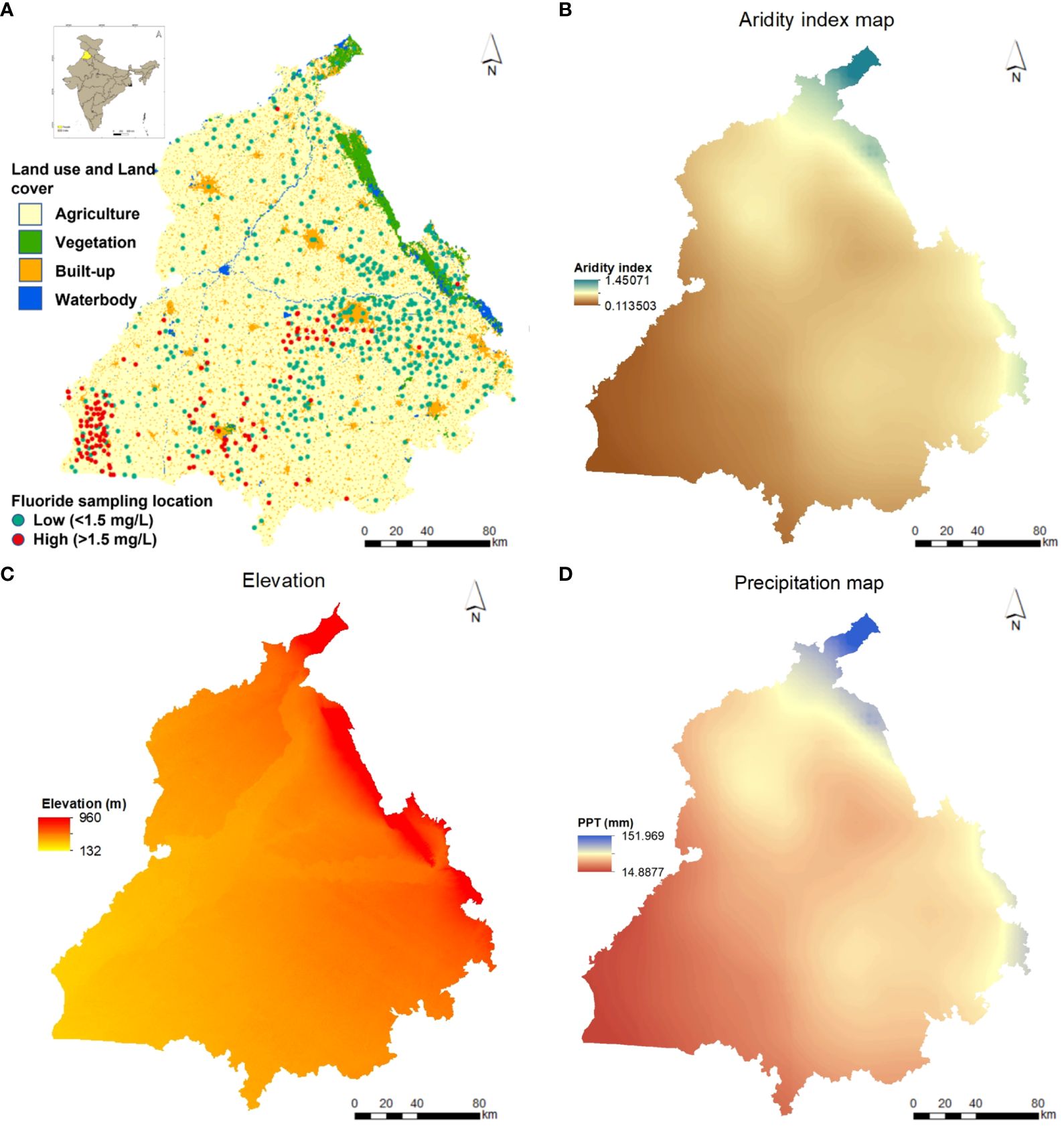
Figure 1 (A) Location map of Punjab showing the land-use and land cover distribution in 2021 (34) along with the fluoride data points at high and low concentrations; (B) aridity (2002); (C) elevation (35); (D) rainfall map of Punjab (36).

3 Materials and methodology

3.1 Data collection, database creation, and processing

Groundwater quality analyses from across the entire state of Punjab were retrieved from various published reports and research articles. We collected a total of 17,317 F⁻ observations: 1,705 data points from Central Groundwater Board (CGWB), 433 observations from Central University of Punjab (CUPB), 745 observations from Duggal and Sharma (41), 11,226 from Khattak et al. (8), 59 observations from Sharma et al. (42), 38 observations from British Geological Survey (BGS) (43), and 3,111 from Department of water supply and sanitation, Punjab government. Besides F⁻, the availability of groundwater physicochemical parameters such as pH, Electrical Conductivity (EC), Total Dissolved Solids (TDS), Chloride (Cl⁻), Nitrate (NO₃⁻), Sulphate (SO₄²⁻), Phosphate (PO₄³⁻), Bicarbonate (HCO₃⁻), Sodium (Na⁺), Potassium (K⁺), Calcium (Ca²⁺), and Magnesium (Mg²⁺) is essential for model development. In conjunction with the groundwater quality determinants, the depth of the collected samples was also considered an important parameter for this study. These variables were selected based on their established or suspected association with the discharge and accumulation of F⁻ in groundwater and were further used to screen the data.

Although these attributes are often measured during groundwater monitoring assessments, some were missing from the datasets collected from different sources. Data collected from research papers (8, 41, 42) did not contain all of this information and, hence, was not included in the final database. In comparison, almost all variables were present in data collected from BGS, CUPB, and CGWB. Although CGWB data was collected from 2013–2015 and 2018–2020 (44–49), only the recent data of the year 2020 was used for prediction modeling. Also, the observations from locations monitored in the previous years but not in 2020 were considered for prediction modeling. This resulted in a total of 298 observations from CGWB. Furthermore, CUPB data consisted of some samples collected from canals and other surface water sources, which were excluded, resulting in a total of 420 data points. Besides the water quality variables and sampling depth, information on the geographical coordinates of the sampling locations was also considered as an essential screening criterion. For sampling points lacking the georeferenced location, Google Earth Pro was used to determine the same by using the name of the sampling location. Therefore, the final database that was finally used for creating a suitable prediction model for groundwater F⁻ concentration contained a total of 756 data points from CGWB, CUPB, and BGS (Figure 1A, Table 1). The final data was also classified into two classes as per the depth at which the samples were collected (optimum depth was considered to be 60 m) (52, 53).

Table 1

Table 1 Detailed information of the groundwater fluoride dataset compiled from different sources.

The values of some of the abovementioned variables were missing in the final dataset, which was estimated with the help of standard formulas. One such missing parameter was TDS in CGWB data that was determined using the following formula (Equations 1, 2) (54):

$\begin{array}{ll}\begin{array}{l}TDS\left(\frac{mg}{L}orppm\right)\hfill \\ =EC\left(\frac{dS}{m}\right)\times 640\left(whenECrangesfrom0.1-5\frac{dS}{m}\right)\hfill \end{array}& (1)\end{array}$

$\begin{array}{ll}\begin{array}{l}TDS\left(\frac{mg}{L}orppm\right)\hfill \\ =EC\left(\frac{dS}{m}\right)\times 800\left(whenECisgreaterthan5\frac{dS}{m}\right)\hfill \end{array}& (2)\end{array}$

Similarly, a few other parameters were reported below their respective detection limit (BDL). These values were then replaced by dividing the BDL value by two. Furthermore, the values of all the parameters were converted to their respective similar unit to ensure uniformity in the dataset. All the anions, cations and TDS were represented in mg/L, EC in µS/cm, and depth in meters, while pH is unitless. Of the final 756 F⁻ measurements, 609 (~81%) were under the permissible limit of 1.5 mg/L, 100 (~13%) ranged from 1.5–3 mg/L, and the remaining 47 (~6%) were greater than 3 mg/L.

3.2 Groundwater hydrochemical characterization and depth distribution

To understand the nature of the distribution of groundwater F⁻ levels and their corresponding physicochemical parameters at different depths, graphical and statistical inference methods were adopted. The compiled dataset was characterized by enumerating its descriptive statistics (minimum, maximum, mean, median, coefficient of variation, first and third quantiles, and percentage of samples exceeding the respective permissible limits). The normality for all the variables was tested using Kolmogorov–Smirnov test. Testing whether the data is normally distributed is necessary, especially for geochemical and other environmental data, because they are generally skewed, consisting of outliers and originating from varied sources (55). Normality testing further aided in selecting the appropriate statistical treatments for the data. Since most parameters are not normally distributed, Spearman’s rank correlation coefficient was enumerated to identify the potential associations of the F⁻ concentrations with the concurrently evaluated physicochemical attributes and sampling depth. All the statistical analyses and graphical plotting were performed in the R software version 4.3.2.

3.3 Model description and development

Machine learning algorithms were further applied to uncover the hidden patterns between the compiled F⁻ concentrations and the physicochemical variables and well depth and develop an optimized model for predicting F⁻ concentration in the study domain. In this study, F⁻ is the output or target (y) variable that will be determined using the input or predictor (x) variables, i.e., the abovementioned physicochemical attributes and the sampling well depth. Five different machine learning models, i.e., Extreme Gradient Boosting (Xgboost), Random Forest (RF), Support Vector Machine (SVM), Extreme Learning Machine (ELM), and Multilayer Perceptron (MLP), were implemented and tested on the final dataset. All of these models have been frequently used in the literature for groundwater-based investigations and, hence, considered for groundwater F⁻ prediction modeling. R software version 4.3.2 was used to develop these proposed models. Before the implementation of these models, a pre-processing step was involved in which data standardization was performed using the Z-score method with the following formula (Equation 3) (56):

$\begin{array}{ll}\acute{x_i}=\frac{x_i-\mu }{\sigma }& (3)\end{array}$

where $\acute{x_i}$ denotes the standardized i^th variable, $x_i$ is the i^th variable, $\sigma$ denotes standard deviation, and $\mu$ is the mean. Following standardization, the entire dataset was randomly shuffled, and a cross-validation technique was employed to further split the data for training and testing the model. 80% of the data was used for training the model, and the remaining 20% was used for validation.

3.3.1 Random Forest

Random Forest is one of the widely recognized and extensively implemented ensemble machine learning methods that has successfully solved real-world issues (56). RF algorithm generates numerous decision trees (hence called a ‘forest’), each of which is built from a random subsample of the data used to train the model (and therefore, the name ‘random’). The algorithm uses the bootstrapping method to select samples randomly, thereby using different combinations of the information in the training dataset. This aids in reducing the semblance among the trees, ultimately making the model more robust. The remaining samples of the input sub-sample set used to train the model are referred to as ‘out of bag’ samples or OOB samples that are utilized for internal cross-validation of the trained model (57). Furthermore, the model opts for a random subset of independent or predictor variables in order to split the data at each node for growing an unbiased tree. The creation of several trees and considering the average number of decisions made for these trees minimizes the problem of overfitting, which is an issue when considering a single decision tree. This aggregation of decisions from different trees enhances the generalization capacity of the Random Forest model (58). To develop an effective RF model, optimization of two hyperparameters, i.e., the total number of trees and the least number of leaf sizes, is required. For this work, four physicochemical parameters as predictor variables were used at each node split. These predictor variables were split by applying a curvature test to grow an unbiased tree. The decision trees count ranged from 1 to 500, and the random search approach was employed for determining the minimum number of leaf sizes.

3.3.2 Support Vector Machine

Support Vector Machine is a structural risk minimization-based statistical learning method that was first proposed by V. N. Vapnik (59). In contrast to the neural network (NN) technique, which may have overfitting and generalization issues, the upper limit of extended risk is reduced in SVM, which enhances its generalization capability (60). Instead of considering a two-dimensional plane, SVM employs hyper-planes to specify decision boundaries between the data observations of distinct classes by using a kernel method (61). An in-depth explanation of the SVM model is given by Ceryan et al. (62). In this study, several kernel functions, such as polynomial, linear, and radial basis kernel functions, were tested, and the best-performing kernel was further selected for prediction. In our study, epsilon value, gamma, and cost were the hyperparameters selected for this model. The epsilon value influences the number of support vectors, which lowers the chances of the model overfitting. In this study, the hyperparameters were optimized by the Bayesian optimization technique, where the Epsilon value was searched in the range of (10⁻³, 10²) and box constraints in the range of (10⁻³, 10³).

3.3.3 Extreme Gradient Boosting

Chen et al. (63) developed the Xgboost model, which is an advanced and improved version of the gradient-boosting machine (GBM). As compared to GBM, Xgboost has a faster learning speed and higher accuracy. It can be employed for both classification and regression problems. It is an ensemble method composed of numerous decision trees where the data splits according to the features. The prediction errors of previous trees are rectified by the addition of new trees for model fitting. Based on the values of the input parameters, each sample is allocated to a set of leaves in a tree that each have a certain numerical weight. The model’s projected output for a particular sample is calculated by adding the sum of the leaves allocated to that sample for each regression tree (64). Step-wise information about Xgboost is provided by Osman et al. (65). In order to achieve better modeling performance and prediction efficiency, it is essential to calculate the optimization parameters. For this study, four hyperparameter algorithms were applied such as Grid Search, Adaptive Random Search, Genetic Algorithm, and Bayesian Optimization, for optimizing the model parameters (nround, eta, lambda, and alpha).

3.3.4 Extreme Learning Machine

ELM is one of the most commonly used ML models due to its incredibly quick learning speed and ability to achieve the minimum training error with the smallest weight norm (66). It is being frequently utilized in various scientific domains such as picture recognition, text classification, biomedicine, environmental forecasting, and others (67–69). ELM is a feedforward neural network that has a single hidden layer between an input layer and an output layer with a strong generalization capacity. Interconnected networks or neurons link the input and hidden layers and also the hidden and output layers. The input weights and biases are generated randomly during the training stage, while the least-square method determines the output weights. Consequently, output weights are established analytically, and therefore, the model is generalized efficiently (66). The performance of this model can be enhanced by optimizing the number of neurons of the intermediate hidden layer and the activation function. In this study, the optimized count of hidden layer neurons was determined by increasing from 1 until the best model was obtained (70). In this study, the activation functions such as rectified linear unit, sigmoid, hard-limit, triangular basis, radial-basis, satlins, and tansig were explored, and the function performing optimally was selected to build the ELM model.

3.3.5 Multilayer Perceptron

Multilayer Perceptron or MLP model is among the most popular neural network models that mimic the human brain for decision-making and problem-solving (71). A comprehensive explanation of the entire model is described by Haykin (64). However, in a nutshell, this model’s structure is composed of an input and output layer with one or more intermediate layers known as hidden layers. The input layer consists of source nodes or neurons that transfer input information to the subsequent hidden layer. Similarly, the hidden layer(s) computes the information provided by the units in the input layer and distributes it further to the output layer. All the input signals are processed by the neurons of hidden and output layers by assigning weights to them. Also, an extra unit known as a bias node is attached to each layer, which primarily generates a signal as an output to the neurons of the current layer. Weights are applied to each input node, which is further integrated and processed by a transfer function that regulates the signal strength discharged through the output nodes (72). Among the various activation functions in MLP architecture, the most frequently used, i.e., the sigmoid activation function, was considered in this study (73). MLP was developed based on a back-propagation technique of the Levenberg–Marquardt (LM) algorithm, which, on further training, acquired the bias and optimal weight (74). The random search method was applied to tune the learning rate of the LM algorithm, which ranged from 0.1–0.9. In this study, a single hidden layer was used to build the MLP model. Also, since the hidden neurons’ count is considered a significant factor in MLP architecture, it was also optimized to prevent the model from overfitting. The number of neurons was tuned by increasing from unity until the model was optimized (70).

3.3.6 Model performance evaluation

The performance of ML models adopted for groundwater F⁻ prediction was assessed using three measures: coefficient of determination (R²), root mean square error (RMSE), and mean absolute error (MAE) (31, 75). R² shows the degree of correlation between two linearly related variables. If the value is close to 1, it indicates a good correlation between the predicted and observed values. Contrarily, RMSE and MAE values close to zero would indicate an excellent fit between the predicted and observed values. The equations for all the three statistical performance measures are provided as follows (Equations 4–6) (76, 77):

$\begin{array}{ll}{R}^2={[{\displaystyle {\sum }_{i=1}^N(P_i-\overline{P})(O_i-\overline{O})}]}^2{[{\displaystyle {\sum }_{i=1}^N{(P_i-\overline{P})}^2{(O_i-\overline{O})}^2}]}^{-1}& (4)\end{array}$

$\begin{array}{ll}RMSE={[N^{-1}{\displaystyle {\sum }_{i=1}^N{(P_i-O_i)}^2}]}^{0.5}& (5)\end{array}$

$\begin{array}{ll}MAE=\frac{1}{N}{\displaystyle {\sum }_{i=1}^N\left|P_i-O_i\right|}& (6)\end{array}$

where N is the total number of observed data, predicted and observed values are denoted by $P_i$ and $O_i$, respectively, and the average of the predicted and observed values are given as $\overline{P}$ and $\overline{O}$, respectively. The entire methodology has been summarized in Figure 2.

Figure 2

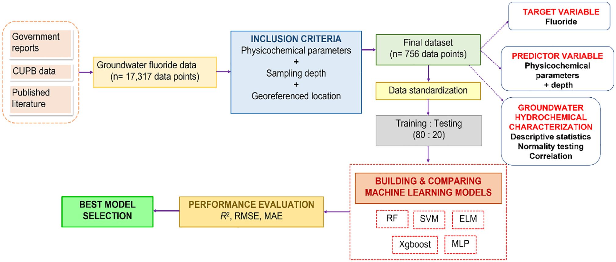
Figure 2 Flow diagram demonstrating the methodology applied for groundwater fluoride database creation and the comparison of different machine-learning models to predict fluoride concentration.

3.3.7 Determination of variable importance

The influence of different explanatory variables on the model’s performance was determined using the ‘varImp’ function of the ‘caret’ package in the R environment. This commonly used function helps rank all the input variables with a standardized measure of importance ranging from 0–100%.

4 Results

4.1 Hydrochemical characterization

Knowledge of the hydrochemical conditions of groundwater is indispensable for identifying potential contaminants to safeguard human health. The descriptive statistics for summarizing the hydrochemical characteristics of the groundwater samples compiled from different sources for this study are presented in Table 2. The pH value for the entire dataset ranged from 6.0 to 9.1 (Table 2), with median values of 8.05 and 7.33 at depths within and exceeding 60 meters (Figure 3), respectively, indicating the predominance of alkaline conditions in the aquifers of this region. Likewise, EC and TDS ranged from 41–16,760 μS cm⁻¹ and 29–13,408 mg/L (Table 2), respectively, with median values higher in shallow (809 μS cm⁻¹ and 531.6 mg L⁻¹, respectively) than in deeper (601 μS cm⁻¹ and 419.2 mg L⁻¹, respectively) waters (Figure 3). According to Freeze and Cherry’s groundwater classification (78), shallow groundwaters in Punjab can be majorly considered as brackish (1000 < TDS < 10000 mg L⁻¹), while deeper waters are classified as freshwater (TDS <1000 mg L⁻¹). Furthermore, the results also show the occurrence of both cations and anions in excess, particularly in shallow depths. Dominant cations in shallow groundwater include Ca²⁺, Mg²⁺, Na⁺, and K⁺, and anions such as Cl⁻, NO₃⁻, SO₄²⁻, F⁻, and HCO₃⁻, whereas, in deeper waters were Mg²⁺, Na⁺, Cl⁻, and HCO₃⁻. Based on overall median concentrations, the cations and anions were arranged in the following order: Na⁺ > Mg²⁺ > Ca²⁺ > K⁺ and HCO₃⁻ > Cl⁻ > SO₄²⁻ > NO₃⁻ > F⁻ > PO₄³⁻, respectively. Furthermore, it was also observed that the median concentrations of Cl⁻, NO₃⁻, SO₄²⁻, Mg²⁺, Na⁺, Ca²⁺, and K⁺ were also elevated in shallow waters compared to deeper waters. The median values of Mg²⁺ and F⁻ were slightly higher in deeper waters than in shallow aquifers (Mg²⁺: 35 and 34.39 mg L⁻¹, respectively; F⁻: 0.71 and 0.57 mg L⁻¹, respectively). Similarly, the median concentration of HCO₃⁻ was much higher in deeper waters than in shallow waters. Therefore, it is evident that the majority of the ions, along with other water quality parameters, are in excess in the shallow aquifers than the deeper groundwater (Figure 3).

Table 2

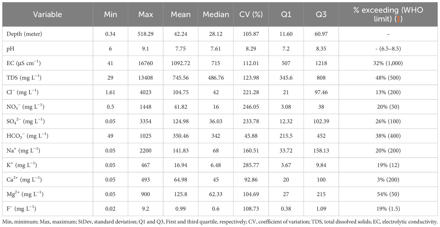
Table 2 Descriptive statistics for characterization of fluoride (F⁻) and concurrently measured physicochemical variables in the alluvial aquifer of Punjab.

Figure 3

Figure 3 Box plots showing the variations in groundwater physicochemical parameters and F⁻ concentration in shallow (< 60 meters) and deeper (> 60 meters) aquifers.

All the hydrochemical parameters except pH displayed a greater degree of coefficient of variation [CV (%)] (Table 2), as well. This clearly implies a wide range of variability within each of the water quality parameters in the study region, arising from various natural sub-surface and surface phenomena and anthropogenic influences. In addition to this, the physicochemical attributes of most of the groundwater samples, particularly sampled from the shallow aquifers, exceeded the recommended safe limit by the World Health Organization (1) (Table 2). The overall percentage of samples exceeding their respective permissible limit for each parameter is as follows (total % exceeding/% exceeding in shallow groundwater samples): EC: 32%/29%; TDS: 48%/40%; Cl⁻: 13%/12%; NO₃⁻: 20%/18%; SO₄²⁻: 26%/24%; HCO₃⁻: 38%/24%; Na⁺: 20%/18%; K⁺: 19%/17%; Ca²⁺: 3%/2.6%; Mg²⁺: 54%/34%; F⁻: 19%/15%.

Furthermore, the Kolmogorov–Smirnov test verified that all the groundwater quality variables did not follow a normal distribution. In shallow waters, F⁻ had a weak to moderate positive correlation with almost all the variables except Ca²⁺. The Spearman’s rank correlation coefficients of F⁻ with all the variables are: Depth = 0.14 (p<0.01); pH = -0.23 (p<0.01); EC = 0.41 (p<0.01); TDS = 0.44 (p<0.01); Cl⁻ = 0.31 (p<0.01); NO₃⁻ = 0.14 (p<0.01); SO₄²⁻ = 0.35 (p<0.01); HCO₃⁻ = 0.34 (p<0.01); Na⁺ = 0.30 (p<0.01); K⁺ = 0.22 (p<0.01); Mg²⁺ = 0.31 (p<0.01); Ca²⁺ = 0.05 (p>0.01). EC and TDS had the highest influence on F⁻ concentration, thus indicating an increase in its concentration with an increase of these parameters.

4.2 Predictive performance evaluation of models

The utilization of groundwater physicochemical parameters as predictor variables for forecasting F⁻ contamination levels through ML approaches has been well established (31). In this study, five different models with diverse architectures, such as RF, SVM, Xgboost, ELM, and MLP, were employed for predicting the groundwater fluoride concentration in the aquifers of Punjab. The model performance was evaluated based on the R², RMSE, and MAE values. These are some of the commonly used metrics for determining the predictive ability of ML models. In the case of the Xgboost model, the Adaptive random search function among the other functions had the highest R² value and the lowest RMSE and MAE values in the testing stage (Table 3). This implies that the Adaptive random search function is the best activation function for Xgboost in the current study, which was further considered for comparing the prediction performance with all the proposed models. For SVM, the radial basis kernel function (RBF) performed better than polynomial, sigmoid, and linear kernel functions as it can handle non-linear datasets (31) and, therefore, selected for prediction purposes in our study. This superior performance of RBF over other kernel functions was also confirmed by Rajasekaran et al. (79), Wu and Wang (80), Amirmojahedi et al. (81). Also, among the various activation functions in the ELM model, the ‘tansig’ function had the most satisfactory output and, therefore, was selected for further prediction-performance comparison between the selected models.

Table 3

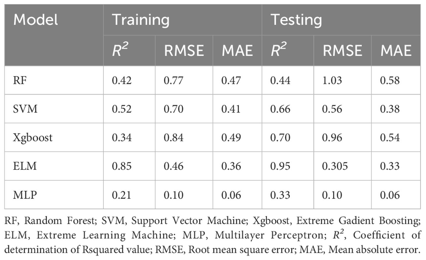
Table 3 Performance measures in the testing and training stages of proposed models.

The overall statistical evaluation criteria for all the models yielded poor to satisfactory results, implying that a few models outperformed others in predicting the F⁻ levels. Based on the 80% of the total dataset used for training purpose, the R² achieved for different models are 0.42 (RF), 0.52 (SVM), 0.34 (Xgboost), 0.85 (ELM), and 0.21 (MLP) (Table 3). Ideally, R² close to unity display greater proximity between the observed and simulated values. Although R² provides an indication of how well the model fits the data, with values close to 1 implying a better fit, it does not provide information about the magnitude of the errors between the actual and predicted values. Hence, RMSE and MAE values were computed along with R² to assess the performance of the different ML models. The RMSE values were 0.77 (RF), 0.70 (SVM), 0.84 (Xgboost), 0.46 (ELM), and 0.10 (ML), and MAE was 0.47 (RF), 0.41 (SVM), 0.49 (Xgboost), 0.36 (ELM), and 0.06 (MLP). Both RMSE and MAE values closer to 0 suggest little error between the actual and predicted values. Based on these values in the testing stage, MLP had the least amount of error followed by ELM, SVM, RF, and Xgboost. Despite the lowest RMSE and MAE values, MLP had the lowest R², suggesting unreliable performance for F⁻ determination in this study. Furthermore, RF also trained very poorly, which is evident from the low R² and significantly greater RMSE and MAE. In addition to MLP and RF, SVM and Xgboost were also trained unsatisfactorily as per the R², RMSE, and MAE values. On the contrary, relatively lower MAE and RMSE values and greater R² value of the ELM model indicates superior training ability relative to the other four models.

After model training, the remaining 20% of the dataset was utilized for testing the model, and the same evaluation metrics were applied to analyze each model’s predictability. The trend of the performance evaluation criteria for all the models was almost similar. The order of the proposed models in terms of the R² values was ELM (0.95) > Xgboost (0.70) > SVM (0.66) > RF (0.44) > MLP (0.33) (Table 3). Satisfactory R² values were observed for ELM, Xgboost, and SVM. Furthermore, error metrics RMSE and MAE for MLP were 0.10 and 0.06, respectively, which were the least among all the models. However, the lowest R² value for MLP obtained from the trained data implies poor model performance and proved unreliable for groundwater fluoride prediction in this region. After MLP, the RMSE (0.31) and MAE (0.33) values for ELM in the testing phase were minimal among the remaining models, emphasizing good prediction ability. From comparing the statistical performance metrics of the training and testing stages of different models, it is evident that only ELM had the optimum values and can be considered for modeling F⁻ concentrations in Punjab. It is noteworthy that MLP and ELM have relatively less complex topology and training algorithms than the remaining three models (30). Nevertheless, their performance varied greatly in predicting the groundwater fluoride concentration in the study domain.

In order to better comprehend the accuracy of model prediction, the observed F⁻ concentrations and their corresponding predicted values after model training were plotted in a scatter diagram (Figure 4). From Figure 4, it is quite evident that the distribution of predicted F⁻ values in relation to the observed F⁻ concentrations is quite closely placed to the best fitting line as opposed to other models, which validates the robustness of the ELM model. Besides ELM, the predicted values of SVM, Xgboost, RF, and MLP did not closely match the actual values, which is substantiated by poor R² values (Figure 4).

Figure 4

Figure 4 Observed versus predicted fluoride (F⁻) concentrations in groundwater for the test data of ELM, SVM, Xgboost, RF, and MLP models. (ELM: Extreme Learning Machine; SVM: Support Vector Machine; Xgboost: Extreme Gradient Boosting; RF: Random Forest; MLP: Multilayer Perceptron).

Spatial distribution maps were prepared to better visualize the actual and predicted F⁻ concentration values for all five models (Figure 5). The predicted values of ELM, Xgboost, SVM, RF, and MLP were compared with the original F⁻ concentrations, and a significant difference between the model outcomes was noted. The south and southwestern regions of Punjab have elevated F⁻ levels (> 1.5 mg/L) in its groundwater system (Figure 5A), whereas the remaining areas exhibited relatively lower concentrations. A significantly similar F⁻ distribution pattern of the ELM predicted values (Figure 5B) with the original F⁻ concentrations was observed, implying a substantial prediction accuracy. Central Punjab had concentrations ranging between 0.5–1.0 mg/L, with parts of northwestern districts having groundwater fluoride surpassing 1.5 mg/L, identical to the original F⁻ distribution and ELM predicted map. Furthermore, based on the concentration values predicted by the remaining four models, excess F⁻ levels were evident across the entire Punjab state. Although central and northern regions had relatively safe groundwater fluoride levels (< 1.5 mg/L) (Figure 5A), contradictory F⁻ distribution as per the predicted values of Xgboost, SVM, RF, and MLP was observed (Figures 5C–F), implying poor model performance. Also, the regions falling in the south and southwest had a greater magnitude of F⁻ content than the original F⁻ levels, indicating an overestimation of excess contaminant levels. These spatial distribution maps of the proposed ML models, in comparison to the original F⁻ distribution, are evidently in accordance with the performance evaluation metrics, i.e., R², RMSE, and MAE (Table 3, Figure 4). Consequently, it can be stated that ELM outperformed the remaining four models in groundwater fluoride levels in the study region.

Figure 5

Figure 5 Spatial comparison of observed F⁻ concentration values with the model predicted F⁻ concentration values. (A) Observed F⁻ concentration; (B) ELM predicted F⁻ concentration; (C) Xgboost predicted F⁻ concentration; (D) SVM predicted F⁻ concentration; (E) RF predicted F⁻ concentration; (F) MLP predicted F⁻ concentration.

4.3 Variable importance by ML models

The predictor (input) variables govern the robustness and stability of the prediction models (82, 83), and therefore, the relative importance ranking of these variables aid in determining the significant variables or factors influencing the contamination. The ranking of the variables was found to be consistent in ELM and SVM (Figure 6), while other models displayed certain variations. In both ELM and SVM, the variables contributing the most to model prediction were TDS, EC, Cl⁻, Na⁺, and Ca²⁺, each with relative importance greater than 15% (Figure 6). These variables also displayed a significant correlation with F⁻. Based on the relative importance scores, TDS, EC, and Na⁺ were the top three variables in these two models in the order TDS > EC > Na⁺, indicating their potential role in mobilizing and enhancing F⁻ in the groundwater of the study domain, particularly in the shallow aquifers. The variable importance of the abovementioned factors was also observed to be significant in the remaining three models; however, it was not in the same order as ELM and SVM. Based on the relative importance scores, the order of the variables was EC > TDS > Na⁺ in Xgboost, TDS > Na⁺ > EC in RF, whereas EC > Ca²⁺ > Na⁺ > TDS in MLP was observed. The relative importance of Cl⁻ and Ca²⁺ ranked 4^th and 5^th in ELM, SVM, and RF, while Xgboost (Ca²⁺ and Cl⁻ ranking 4^th and 5^th, respectively) and MLP (Ca²⁺ and Cl⁻ ranking 2^nd and 5^th, respectively) displayed slight variation. The variable SO₄²⁻ attained the least importance in ELM (0.5), SVM (0.2), Xgboost (1.1), RF (0.3), and MLP (0.3) (Figure 6). The ranking discrepancies between these variables in all the five models could have resulted due to the differences in model algorithms (24).

Figure 6

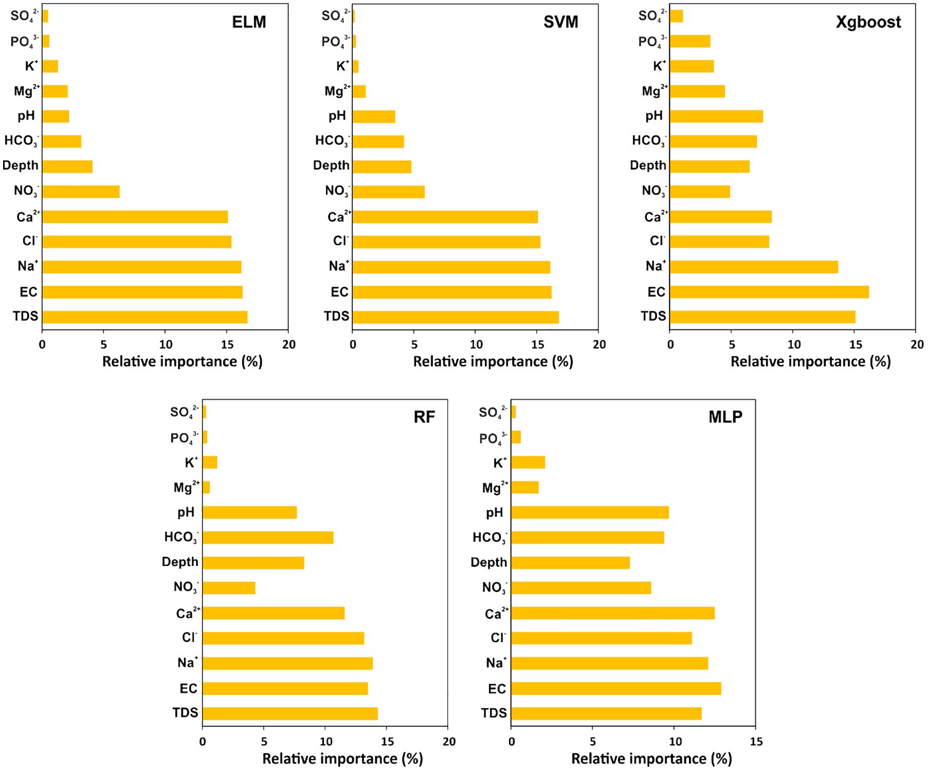
Figure 6 Relative importance ranking of hydrochemical parameters for ELM, SVM, Xgboost, RF, and MLP models. (ELM: Extreme Learning Machine; SVM: Support Vector Machine; Xgboost: Extreme Gradient Boosting; RF: Random Forest; MLP: Multilayer Perceptron).

5 Discussion

5.1 Groundwater fluoride and other physicochemical characteristics

The occurrence of elevated F⁻ concentrations in the groundwater of the Punjab basin is attributed mainly to geogenic origin (84), which results from the interplay of multiple complex interdependent hydrogeochemical processes (85). Naturally occurring F⁻ in minerals and rocks are nearly insoluble in water. However, favorable conditions facilitate the dissolution of these minerals, further releasing F⁻ into the groundwater (86). Dissolution of fluoride-bearing minerals, in particular fluorite, under suitable conditions, such as alkaline pH with excess EC and TDS, as observed in the aquifers of Punjab, favors F⁻ enrichment. The alkaline nature of the groundwater could be attributed to the presence of sediments containing abundant carbonate minerals (85). Elevated EC and TDS could be a consequence of the rapid and greater degree of rock and mineral weathering, waterlogging, and dissolution of salts (17, 56). Furthermore, anthropogenic inputs from agricultural and industrial practices and groundwater recharge through shallow aquifers also contribute to high EC and TDS (87). An increase in EC and TDS elevates the water’s ionic strength and major ion concentration. This results in a greater competitive effect between ions and F⁻ from soil exchange sites and mineral surfaces through the ion exchange process, thus reducing the adsorption potential of F⁻ and enhancing their mobilization (84, 88). Sodium and chloride ions, responsible for TDS/EC, also significantly correlated with F⁻. Calcite precipitation (decrease in Ca²⁺) enriches F⁻ in the groundwaters, hence the negative correlation between the two. Also, F⁻ and all other hydrochemical parameters in shallow aquifers surpassed their respective permissible limits compared to the deeper water samples. Shallow waters are easily accessible for human consumption and other activities, and therefore, raises concern over affecting human well-being.

Besides the groundwater hydrogeochemical conditions, the prevailing arid and semi-arid climate in the study region increases evaporation rates relative to humid areas. High rainfall inputs and subsequent dilution effect in humid climatic zones result in lower groundwater fluoride levels compared to drier environments. Also, the groundwater movement in arid/semi-arid regions is generally slow, thereby increasing the contact time between the water and rock, which further causes F⁻ enrichment in water (85, 89).

5.2 Model output and performance

Excess groundwater fluoride incidence in arid and semi-arid regions is a common phenomenon (90, 91), as observed in the aquifers of Punjab. Furthermore, due to its geogenic origin, the concentration of F⁻ depends directly on the hydrogeochemical conditions. Also, relatively limited studies have forecast F⁻ levels in arid and semi-arid locations using hydrochemical characteristics. Therefore, developing a predictive model for determining F⁻ levels using water quality variables in locations lacking monitoring assessments is essential. This study proposed five different ML models (RF, MLP, SVM, ELM, and Xgboost) and determined the best-performing model based on the evaluation metrics (R², RMSE, and MAE). Out of all the models, MLP trained extremely poorly for the dataset and is, therefore, unsuitable for making reliable predictions of groundwater fluoride concentration in our study area. This finding is contrary to Nafouanti et al. (28) and Gupta and Maiti (30), where MLP performed accurately in predicting F⁻ concentrations in the Datong basin (China) and Maharashtra (India), respectively. The poor performance of MLP in our study could be due to its incapability to extrapolate beyond the data used for training, which further leads to overfitting issues during the training phase (92, 93). The worst prediction performing model in both the training and testing stages was MLP, which contradicts Bui et al. (94). The MLP is based on neural network architecture that can generate more accurate results on a badly structured dataset than on tree-based models such as RF (94). On the contrary, the RF model overcomes overfitting issues by combining many trees, thereby free from bias, resulting in enhanced prediction performance (32). Regardless, RF performed poorly in the training phase as well. Both MLP and RF generated values that deviated greatly from the original values, implying unsatisfactory performance. MLP tends to overfit from the training data, interfering with its ability to infer the remaining data (test/cross-validation dataset) (28). Gupta and Maiti (30), in their work, also stated that MLP, RF, and SVM are less effective in uncovering the intricate non-linear association between the target and predictor variables. Unsatisfactory training values of MLP, RF, SVM, and Xgboost could have resulted from a very wide variability in the range of both the target (output) and predictor (input) variables within the compiled dataset. This adds a limitation to model fitting in our study, resulting in inaccurate prediction results. Data pre-treatment involving outlier suppression and logarithmic transformation can be a possible solution to further improve the prediction accuracies (30). However, these pre-processing steps on the raw dataset and their influence on the model performance need further evaluation. Gupta and Maiti (30) also emphasized on the limited prediction efficiency of the ELM model due to its design and direct inverse in estimating the bias and weights. Irrespective of this fact, the ELM model with relatively higher R² value and low RMSE and MAE values in the training phase in comparison to the remaining models implies good generalization capability for our dataset without undergoing much pre-processing, unlike other models tested in this study.

Classification-based ML models have been commonly used in groundwater fluoride level prediction (10, 26, 27, 95, 96), with very few studies on regression-based prediction modeling of the same (30, 31). The complexity and accuracy of the datasets, diverse algorithm architectures, and type and number of input parameters significantly influence the performance of the models, and therefore, there is no universal agreement on which ML model performs the best for all prediction-related studies (94). For instance, groundwater fluoride concentration in the Datong basin, China, was modelled using RF, Linear regression (LR), and MLP-based Artificial neural network (ANN), where RF proved to be the best prediction model (28). Similarly, the RF model displayed higher prediction accuracy for other contaminants, such as nitrate, than the enhanced regression tree, classified regression tree, and multiple linear regression (97). Khosravi et al. (98), instead, reported that the M5P model had the highest predictive power than Instance Based Learner (IBK), KStar, Locally Weighted Learning (LWL), and Regression by discretization (RBD) that were tested for predicting F⁻ in the aquifers of Maku plain in Iran. Similarly, F⁻ levels in the groundwater of Sindhudurg district in Maharashtra, India, were predicted using six different models, out of which ELM yielded the most unsatisfactory results (30). On the contrary, Barzegar et al. (31) compared the performance of three different models and determined ELM to be the best for forecasting F⁻ in the Maku Valley of Iran, which is in accordance with the findings of the current study. Therefore, it is advisable to test diverse algorithms with the same dataset and assess their performance in terms of prediction before selecting the best.

The ELM model has a simple architecture and an uncomplicated training process and is generally known for its efficient computational power, requiring fewer hyperparameters for model tuning and training. The parameters of the hidden layer in this model do not require manual adjustments and are also independent of the input data. It only determines the weights of the output analytically and thus has rapid learning speed and lower computation complexity (99) than the other models proposed in this work. Additionally, ELM also has good generalization capability for high dimensional datasets by initialization of weights and biases stochastically to avoid overfitting problems and thus making the model more robust (100). The superior predictive performance of ELM over other models was also confirmed in other works (69, 101–104).

It is worth nothing that most of the studies conducted in the Indian subcontinent have reported RF and MLP to be the best models for predicting F⁻ concentrations in groundwater. However, these models did not take into consideration the groundwater-physicochemical parameters and used only continuous variables such as climate, soil, geological, and topological parameters as predictors (10, 27, 96). Machine learning algorithms are designed to perform both classification and regression-related tasks. Classification-based ML models have been commonly applied for studies in India that facilitated in forecasting the contamination-risk prone areas (105–107). Nevertheless, it is equally essential to develop models for predicting the concentration of the contaminants based on the driving factors that directly influence its enhancement and mobility. In this context, regression-based modeling will prove to be much more beneficial than classification models. This study attempted to achieve this goal; therefore, such contrasting results could be due to these reasons.

5.3 Hydrochemical drivers affecting the model performance

The different variables influencing groundwater fluoride contamination in any region are complex and require an in-depth understanding to identify the potential parameters for proper groundwater resource management. The variable importance ranking in the present work highlighted that TDS, EC, Na⁺, Cl⁻, and Ca²⁺ were the most crucial factors and were highly correlated with F⁻ content in the study region. The increase in TDS and EC results in increased ionic strength and higher concentration of major ions dissolved in water. These factors enhance competition between ions and F⁻ from mineral surfaces and soil exchange sites through the ion-exchange process, which further minimizes the adsorption of F⁻ and makes them more mobile (84, 88). Sodium, one of the important parameters responsible for EC and TDS, forms compounds with F⁻, such as NaF, which further dissolves in water and becomes more mobile (108). Other factors, such as Cl⁻ and Ca²⁺, contributed significantly to the model performance at varying degrees. The primary source of F⁻ in this region is fluorite mineral (CaF₂), which undergoes dissolution further releasing F⁻ and Ca²⁺ and the latter precipitates in the presence of excess bicarbonate (HCO₃⁻), thereby resulting in free F⁻ ions (109). On the contrary, the chloride ion undergoes ionic exchange with F⁻ from the aquifer substrate, bringing about the discharge of F⁻ ions from these surfaces. Furthermore, the significant contributions of the top 5 variables, i.e., TDS, EC, Na⁺, Cl⁻, and Ca²⁺, in all the five models, irrespective of their prediction accuracies, indicate their potential in determining F⁻ levels in regions lacking groundwater quality monitoring practices. However, the variability in the accuracy post-tuning of the different models might have impacted the outcomes. In other words, data quality, input parameters, hyperparameter tuning process, and varying algorithm architecture play a significant role in the prediction of the target variable. Moreover, the top contributors and their influence on groundwater F⁻ concentration are clearly highlighted from their relative importance scores in all the models, particularly in the ELM model (Figure 6). In addition to this, the maximum prediction accuracy of ELM relative to other proposed models (Table 3, Figures 4, 5) makes it an acceptable method for groundwater quality assessment investigations.

6 Limitations and future research directions

The study compiled a huge amount of data from different sources, introducing varying degrees of discrepancies within the complete dataset. Diverse analytical techniques and procedures might have been adopted in determining F⁻ and the other water quality parameters among the different data sources, affecting the consistency within the final dataset. In addition to this, the seasonal factor, which plays a key role in the contaminant levels in the aquifers, was not considered as a screening criterion in our study. A small proportion of values of certain variables were missing in the complete dataset, which was estimated based on established formulae reported in the literature. All of these factors might have introduced some inconsistencies within the data, which were ultimately used for prediction modeling. Furthermore, the number of samples within each district of the state of Punjab varied greatly, providing an incomplete picture of the study region. Also, the outlier impact post data treatment was also still quite significant. Therefore, the predictive performance of the models might have been affected by all of these factors. The resulting uncertainty among the different models might have originated from the amount of data and noise within the data and variables. The number of variables might have affected the performance of the models. Yet, the results obtained offer satisfactory results regarding a reliable F⁻ prediction model, i.e., ELM. This model accurately captures the role of the different hydrochemical parameters and delivers precise concentration values, proving to be reliable for groundwater fluoride estimation in the region.

This study highlights the significant role of outliers in impacting the prediction model performance. This implies the further need for data pre-processing for environmental datasets that often exhibit non-normal distribution. De-noising and efficient data transformation methods should be explored to enhance the data quality and predictive performance. Furthermore, more advanced and hybrid models can be applied to this kind of dataset to build a more robust contamination prediction system. The prediction performance of the models based on the varying number of potential input variables should also be assessed to enhance its applicability. These same models can also be tested for other groundwater contaminants and compared to determine the best predictive model. As mentioned earlier, classification-based ML modeling for groundwater contaminants, including F⁻, is commonly applied with very limited work on regression-based contaminant concentration modeling. Therefore, this issue should be addressed more, particularly in the Indian sub-continent, where various locations exist without any monitoring assessments.

7 Conclusion

In this work, a comparative performance ability of five different models for predicting F⁻ concentrations in the alluvial aquifers of Punjab was assessed. Models including ELM, SVM, MLP, RF, and Xgboost models were developed, and performance was evaluated using R², RMSE, and MAE. Except for ELM, the remaining four models performed very poorly both during the training and testing phases. Excess variability within the target and predictor variables post data normalization might have impacted the model performance. Although ELM performed satisfactorily, it can be improved with the further pre-treatment of the dataset. Hybrid models can also produce superior prediction accuracy for such complicated environmental problems that need to be explored. Furthermore, similar regression-based modeling studies should be conducted to thoroughly understand the groundwater fluoride problem. Input variables such as TDS, EC, Na⁺, Cl⁻, and Ca²⁺ contributed significantly to the model performance. Evidently, the dynamics of groundwater chemistry are highly complex and vary from location to location. The groundwater fluoride prediction based on the corresponding water quality parameters is crucial for sustainable groundwater management, planning, and further safeguarding human health. Therefore, it is essential to build robust non-linear models to resolve this problem efficiently.

Data availability statement

The original contributions presented in the study are included in the article/supplementary material. Further inquiries can be directed to the corresponding author/s.

Author contributions

AK: Data curation, Formal analysis, Methodology, Software, Visualization, Writing – original draft. PKS: Methodology, Supervision, Writing – review & editing. HSK: Methodology, Software, Supervision, Writing – review & editing.

Funding

The author(s) declare financial support was received for the research, authorship, and/or publication of this article. AK would like to thank the University Grant Commission (UGC: 3810/(NET-JULY2018)), Government of India, for providing financial support in terms of the research fellowship. PKS sincerely acknowledges DST SERB New Delhi (Government of India) for providing support to this work through core research grant (CRG/2021/002567). We would also like to thank the DST-FIST lab at the Department of Environmental Science and Technology, Central University of Punjab for technical support. HSK also acknowledges the DST FIST (SR/FST/MS-I/2021/104) for supporting this work.

Conflict of interest

The authors declare that the research was conducted in the absence of any commercial or financial relationships that could be construed as a potential conflict of interest.

The author(s) declared that they were an editorial board member of Frontiers, at the time of submission. This had no impact on the peer review process and the final decision.

Publisher’s note

All claims expressed in this article are solely those of the authors and do not necessarily represent those of their affiliated organizations, or those of the publisher, the editors and the reviewers. Any product that may be evaluated in this article, or claim that may be made by its manufacturer, is not guaranteed or endorsed by the publisher.

References

1. WHO. Guidelines for drinking water quality Vol. 1. Geneva, Switzerland: World Health Organization (2011).

Google Scholar

2. Neisi A, Mirzabeygi M, Zeyduni G, Hamzezadeh A, Jalili D, Abbasnia A, et al. Data on fluoride concentration levels in cold and warm season in City area of Sistan and Baluchistan Province, Iran. Data Brief. (2018) 18:713–8. doi: 10.1016/j.dib.2018.03.060

PubMed Abstract | CrossRef Full Text | Google Scholar

3. Ashrafi SD, Jaafari J, Sattari L, Esmaeilzadeh N, Safari GH. Monitoring and health risk assessment of fluoride in drinking water of East Azerbaijan Province, Iran. Int J Environ Anal Chem. (2020) 103:1–15. doi: 10.1080/03067319.2020.1849662

CrossRef Full Text | Google Scholar

4. Ayoob S, Gupta AK. Fluoride in drinking water: A review on the status and stress effects. Crit Rev Environ Sci Technol. (2006) 36:433–87. doi: 10.1080/10643380600678112

CrossRef Full Text | Google Scholar

5. Mukherjee I, Singh UK. Groundwater fluoride contamination, probable release, and containment mechanisms: a review on Indian context. Environ Geochem Health. (2018) 40:2259–301. doi: 10.1007/s10653-018-0096-x

PubMed Abstract | CrossRef Full Text | Google Scholar

6. Chakraborti D, Rahman MM, Chatterjee A, Das D, Das B, Nayak B, et al. Fate of over 480 million inhabitants living in arsenic and fluoride endemic Indian districts: Magnitude, health, socio-economic effects and mitigation approaches. J Trace Elem Med Biol. (2016) 38:33–45. doi: 10.1016/j.jtemb.2016.05.001

PubMed Abstract | CrossRef Full Text | Google Scholar

7. Chakraborti D, Das B, Murrill MT. Examining India’s groundwater quality management. Environ Sci Technol. (2011) 45:27–33. doi: 10.1021/es101695d

PubMed Abstract | CrossRef Full Text | Google Scholar

8. Khattak JA, Farooqi A, Hussain I, Kumar A, Singh CK, Mailloux BJ, et al. Groundwater fluoride across the Punjab plains of Pakistan and India: Distribution and underlying mechanisms. Sci Total Environ. (2022) 806:151353. doi: 10.1016/j.scitotenv.2021.151353

PubMed Abstract | CrossRef Full Text | Google Scholar

9. Rasool A, Farooqi A, Xiao T, Ali W, Noor S, Abiola O, et al. A review of global outlook on fluoride contamination in groundwater with prominence on the Pakistan current situation. Environ Geochem Health (2018) 40:1265–81. doi: 10.1007/s10653-017-0054-z

PubMed Abstract | CrossRef Full Text | Google Scholar

10. Podgorski JE, Labhasetwar P, Saha D, Berg M. Prediction modeling and mapping of groundwater fluoride contamination throughout India. Environ Sci Technol. (2018) 52:9889–98. doi: 10.1021/acs.est.8b01679

PubMed Abstract | CrossRef Full Text | Google Scholar

11. Ali W, Aslam MW, Junaid M, Ali K, Guo Y, Rasool A, et al. Elucidating various geochemical mechanisms drive fluoride contamination in unconfined aquifers along the major rivers in Sindh and Punjab, Pakistan. Environ Pollut. (2019) 249:535–49. doi: 10.1016/j.envpol.2019.03.043

PubMed Abstract | CrossRef Full Text | Google Scholar

12. Kumar M, Goswami R, Patel AK, Srivastava M, Das N. Scenario, perspectives and mechanism of arsenic and fluoride Co-occurrence in the groundwater: A review. Chemosphere. (2020) 249:126126. doi: 10.1016/j.chemosphere.2020.126126

PubMed Abstract | CrossRef Full Text | Google Scholar

13. Jaswal V, Kumar R, Sahoo PK, Mittal S, Kumar A, Sahoo SK, et al. Multi-parametric groundwater quality and human health risk assessment vis-à-vis hydrogeochemical process in an Agri-intensive region of Indus basin, Punjab, India. Toxin Rev. (2022) 41:768–84. doi: 10.1080/15569543.2021.1929324

CrossRef Full Text | Google Scholar

14. Rishi MS, Keesari T, Sharma DA, Pant D, Sinha UK. Spatial trends in uranium distribution in groundwaters of Southwest Punjab, India-A hydrochemical perspective. J Radioanalytical Nucl Chem (2017) 311:1937–45. doi: 10.1007/s10967-017-5178-1

CrossRef Full Text | Google Scholar

15. Nizam S, Virk HS, Sen IS. High levels of fluoride in groundwater from Northern parts of Indo-Gangetic plains reveals detrimental fluorosis health risks. Environ Adv (2022) 8:100200. doi: 10.1016/j.envadv.2022.100200

CrossRef Full Text | Google Scholar

16. Krishan G, Kumar B, Sudarsan N, Rao MS, Ghosh NC, Taloor AK, et al. Isotopes (δ18O, δD and 3H) variations in groundwater with emphasis on salinization in the state of Punjab, India. Sci Total Environ. (2021) 789:148051. doi: 10.1016/j.scitotenv.2021.148051

PubMed Abstract | CrossRef Full Text | Google Scholar

17. Sahoo PK, Virk HS, Powell MA, Kumar R, Pattanaik JK, Salomão GN, et al. Meta-analysis of uranium contamination in groundwater of the alluvial plains of Punjab, northwest India: Status, health risk, and hydrogeochemical processes. Sci Total Environ. (2022) 807:151753. doi: 10.1016/j.scitotenv.2021.151753

PubMed Abstract | CrossRef Full Text | Google Scholar

18. Alagha JS, Said MAM, Mogheir Y. Modeling of nitrate concentration in groundwater using artificial intelligence approach-a case study of Gaza coastal aquifer. Environ Monit Assess. (2014) 186:35–45. doi: 10.1007/s10661-013-3353-6

PubMed Abstract | CrossRef Full Text | Google Scholar

19. Saboe D, Ghasemi H, Gao MM, Samardzic M, Hristovski KD, Boscovic D, et al. Real-time monitoring and prediction of water quality parameters and algae concentrations using microbial potentiometric sensor signals and machine learning tools. Sci Total Environ. (2021) 764:142876. doi: 10.1016/j.scitotenv.2020.142876

PubMed Abstract | CrossRef Full Text | Google Scholar

20. Huynh TMT, Ni CF, Su YS, Nguyen VCN, Lee IH, Lin CP, et al. Predicting heavy metal concentrations in shallow aquifer systems based on low-cost physiochemical parameters using machine learning techniques. Int J Environ Res Public Health. (2022) 19:12180. doi: 10.3390/ijerph191912180

PubMed Abstract | CrossRef Full Text | Google Scholar

21. Javadi AA, AL-Najjar MM. Finite element modeling of contaminant transport in soils including the effect of chemical reactions. J Hazard Mater. (2007) 143:690–701. doi: 10.1016/j.jhazmat.2007.01.016

PubMed Abstract | CrossRef Full Text | Google Scholar

22. Ghosh D, Donselaar ME. Predictive geospatial model for arsenic accumulation in Holocene aquifers based on interactions of oxbow-lake biogeochemistry and alluvial geomorphology. Sci Total Environ. (2023) 856:158952. doi: 10.1016/j.scitotenv.2022.158952

PubMed Abstract | CrossRef Full Text | Google Scholar

23. Coppola EA, Rana AJ, Poulton MM, Szidarovszky F, Uhl VW. A neural network model for predicting aquifer water level elevations. Ground Water. (2005) 43:231–41. doi: 10.1111/j.1745-6584.2005.0003.x

PubMed Abstract | CrossRef Full Text | Google Scholar

24. Yang H, Wang P, Chen A, Ye Y, Chen Q, Cui R, et al. Prediction of phosphorus concentrations in shallow groundwater in intensive agricultural regions based on machine learning. Chemosphere. (2023) 313:137623. doi: 10.1016/j.chemosphere.2022.137623

PubMed Abstract | CrossRef Full Text | Google Scholar

25. Cui L, Wang S. Mapping the daily nitrous acid (HONO) concentrations across China during 2006–2017 through ensemble machine-learning algorithm. Sci Total Environ. (2021) 785:147325. doi: 10.1016/j.scitotenv.2021.147325

PubMed Abstract | CrossRef Full Text | Google Scholar

26. Podgorski J, Berg M. Global analysis and prediction of fluoride in groundwater. Nat Commun. (2022) 13:4232. doi: 10.1038/s41467-022-31940-x

PubMed Abstract | CrossRef Full Text | Google Scholar

27. Aind DA, Malakar P, Sarkar S, Mukherjee A. Controls on groundwater fluoride contamination in eastern parts of India: insights from unsaturated zone fluoride profiles and AI-based modeling. Water (Switzerland). (2022) 14:3220. doi: 10.3390/w14203220

CrossRef Full Text | Google Scholar

28. Nafouanti MB, Li J, Mustapha NA, Uwamungu P, AL-Alimi D. Prediction on the fluoride contamination in groundwater at the Datong Basin, Northern China: Comparison of random forest, logistic regression and artificial neural network. Appl Geochem. (2021) 132:105054. doi: 10.1016/j.apgeochem.2021.105054

CrossRef Full Text | Google Scholar

29. Ataş M, Yeşilnacar Mİ, Demir Yetiş A. Novel machine learning techniques based hybrid models (LR-KNN-ANN and SVM) in prediction of dental fluorosis in groundwater. Environ Geochem Health. (2022) 44:3891–905. doi: 10.1007/s10653-021-01148-x

PubMed Abstract | CrossRef Full Text | Google Scholar

30. Gupta PK, Maiti S. Enhancing data-driven modeling of fluoride concentration using new data mining algorithms. Environ Earth Sci. (2022) 81:89. doi: 10.1007/s12665-022-10216-z

CrossRef Full Text | Google Scholar

31. Barzegar R, Asghari Moghaddam A, Adamowski J, Fijani E. Comparison of machine learning models for predicting fluoride contamination in groundwater. Stochastic Environ Res Risk Assess. (2017) 31:2705–18. doi: 10.1007/s00477-016-1338-z

CrossRef Full Text | Google Scholar

32. Nafouanti MB, Li J, Nyakilla EE, Mwakipunda GC, Mulashani A. A novel hybrid random forest linear model approach for forecasting groundwater fluoride contamination. Environ Sci pollut Res. (2023) 30:50661–74. doi: 10.1007/s11356-023-25886-w

CrossRef Full Text | Google Scholar

33. Hundal HS, Kumar R, Singh K, Singh D. Occurrence and geochemistry of arsenic in groundwater of Punjab, northwest India. Commun Soil Sci Plant Anal. (2007) 38:2257–77. doi: 10.1080/00103620701588312

CrossRef Full Text | Google Scholar

34. Esri Microsoft IO. Sentinel-2 10m land Use/Land cover timeseries downloader (Mature support) (2022). Available at: https://www.arcgis.com/home/item.html?id=fc92d38533d440078f17678ebc20e8e2 (Accessed 4th June, 2022).

Google Scholar

35. U.S. Geological Survey. 3D elevation program 1-meter resolution digital elevation model (published 20220439).

Google Scholar

36. Abatzoglou JT, Dobrowski SZ, Parks SA, Hegewisch KC. TerraClimate, a high-resolution global dataset of monthly climate and climatic water balance from 1958-2015. Sci Data. (2018) 5. doi: 10.1038/sdata.2017.191

PubMed Abstract | CrossRef Full Text | Google Scholar

37. Roy PS, Meiyappan P, Joshi PK, Kale MP, Srivastav VK, Srivasatava SK, et al. Decadal land use and land cover classifications across India 1985, 1995, 2005. Ornl Daac. (2016) 7:1–9. doi: 10.3334/ORNLDAAC/1336

CrossRef Full Text | Google Scholar

38. CGWB. Ground Water Year Book Punjab and Chandigarh (UT). (2021) (India: Central Groundwater Board).

Google Scholar

39. CGWB. Concept Note On GEOGENIC CONTAMINATION OF GROUND WATER IN INDIA. India: Central Ground Water Board Ministry of Water Resources Govt. of India (2014) p. 1–99.

Google Scholar

40. CGWB. Uranium occurance in shallow aquifers in India (2020). Available online at: http://cgwb.gov.in/WQ/URANIUM_REPORT_2020.pdf.

Google Scholar

41. Duggal V, Sharma S. Fluoride contamination in drinking water and associated health risk assessment in the Malwa Belt of Punjab, India. Environ Adv. (2022) 8:100242. doi: 10.1016/j.envadv.2022.100242

CrossRef Full Text | Google Scholar

42. Sharma T, Litoria PK, Bajwa BS, Kaur I. Appraisal of groundwater quality and associated risks in Mansa district (Punjab, India). Environ Monit Assess. (2021) 193:159. doi: 10.1007/s10661-021-08892-8

PubMed Abstract | CrossRef Full Text | Google Scholar

43. Lapworth DJ, Krishan G, MacDonald AM, Rao MS. Groundwater quality in the alluvial aquifer system of northwest India: New evidence of the extent of anthropogenic and geogenic contamination. Sci Total Environ. (2017) 599–600:1433–44. doi: 10.1016/j.scitotenv.2017.04.223

PubMed Abstract | CrossRef Full Text | Google Scholar

44. CGWB. Annual Report 2014–15; Central Ground Water Board: Faridabad. India: Government of India (2014).

Google Scholar

45. CGWB. Annual Report 2015–16; Central Ground Water Board: Faridabad. India: Government of India (2015).

Google Scholar

46. CGWB. Annual Report 2018–19; Central Ground Water Board: Faridabad. India: Government of India (2018).

Google Scholar

47. CGWB. Annual Report 2019–20; Central Ground Water Board: Faridabad. India: Government of India (2019).

Google Scholar

48. CGWB. Annual Report 2020–21; Central Ground Water Board: Faridabad. India: Government of India (2020).

Google Scholar

49. CGWB. Annual Report 2013–14; Central Ground Water Board: Faridabad. India: Government of India (2013).

Google Scholar

50. Mittal S, Sahoo PK, Sahoo SK, Kumar R, Tiwari RP. Hydrochemical characteristics and human health risk assessment of groundwater in the Shivalik region of Sutlej basin, Punjab, India. Arab J Geosci. (2021) 14:847. doi: 10.1007/s12517-021-07043-0

CrossRef Full Text | Google Scholar

51. Kumar R, Mittal S, Peechat S, Sahoo PK, Sahoo SK. Quantification of groundwater–agricultural soil quality and associated health risks in the agri-intensive Sutlej River Basin of Punjab, India. Environ Geochem Health. (2020) 42:4245–68. doi: 10.1007/s10653-020-00636-w

PubMed Abstract | CrossRef Full Text | Google Scholar

52. Chopra RPS, Krishan G. Analysis of aquifer characteristics and groundwater quality in southwest punjab, india. J Earth Sci Eng. (2014) 4(10):597–604. doi: 10.17265/2159-581X/2014.10.002

CrossRef Full Text | Google Scholar

53. Bala R, Karanveer, Das D. Occurrence and behaviour of uranium in the groundwater and potential health risk associated in semi-arid region of punjab, india. Groundw Sustain Dev (2022) 17:100731. doi: 10.1016/j.gsd.2022.100731

CrossRef Full Text | Google Scholar

54. Grattan SR. Irrigation Water Salinity and Crop Production. In: Irrigation Water Salinity and Crop Production (2002) (California: ANR Publication). doi: 10.3733/ucanr.8066

CrossRef Full Text | Google Scholar

55. Filzmoser P, Reimann C. Normal and lognormal data distribution in geochemistry : death of a myth. Consequences for the statistical treatment of geochemical and environmental data. Environ Geol. (1999) 39:1001–14. doi: 10.1007/s002549900081

CrossRef Full Text | Google Scholar

56. Singh G, Rishi MS, Herojeet R, Kaur L, Priyanka, Sharma K. Multivariate analysis and geochemical signatures of groundwater in the agricultural dominated taluks of Jalandhar district, Punjab, India. J Geochem Explor. (2020) 208:106395. doi: 10.1016/j.gexplo.2019.106395

CrossRef Full Text | Google Scholar

57. Breiman L. Random forests. Random Forests. (2001) 45:5–32. doi: 10.4324/9781003109396-5

CrossRef Full Text | Google Scholar

58. Prasad AM, Iverson LR, Liaw A. Newer classification and regression tree techniques: Bagging and random forests for ecological prediction. Ecosystems. (2006) 9:181–99. doi: 10.1007/s10021-005-0054-1

CrossRef Full Text | Google Scholar

59. Vapnik VN. The nature of statistical learning theory. New York: Springer (1995). doi: 10.1007/978-1-4757-2440-0

CrossRef Full Text | Google Scholar

60. Gunn S. Support Vector Machines for classification and regression. In: ISIS Technical Report, vol. 14. (1998) (Southampton. U.K.: Image Speech and Intelligent Systems Group). doi: 10.1039/b918972f

CrossRef Full Text | Google Scholar

61. Kecman V. Support Vector Machines: Theory and Applications. In: Springer Science & Business Media, vol. 177. (2005) (Berlin: Springer). Available at: https://books.google.com/books?hl=en&lr=&id=uTzMPJjVjsMC&oi=fnd&pg=PA1&dq=support+vector+machines&ots=GFAK9w2Hfb&sig=4AddZM1BrpsopEIiErlIzeys6zI.

Google Scholar

62. Ceryan N, Ozkat EC, Korkmaz Can N, Ceryan S. Machine learning models to estimate the elastic modulus of weathered magmatic rocks. Environ Earth Sci. (2021) 80:448. doi: 10.1007/s12665-021-09738-9

CrossRef Full Text | Google Scholar

63. Chen T, He T, Benesty M. XGBoost : eXtreme gradient boosting. R Package version 0.71-2. (2018). doi: 10.1145/2939672.2939785

CrossRef Full Text | Google Scholar

64. Haykin S. Neural networks: a comprehensive foundation. United States: Prentice-Hall (1999).

Google Scholar

65. Osman AIA, Ahmed AN, Chow MF, Huang YF, El-Shafie A. Extreme gradient boosting (Xgboost) model to predict the groundwater levels in Selangor Malaysia. Ain Shams Eng J. (2021) 12:1545–56. doi: 10.1016/j.asej.2020.11.011

CrossRef Full Text | Google Scholar

66. Huang G, Zhu QY, Siew CK. Extreme learning machine: Theory and applications. Neurocomputing. (2006) 70:489–501. doi: 10.1016/j.neucom.2005.12.126

CrossRef Full Text | Google Scholar

67. Ali S, Li J, Pei Y, Aslam MS, Shaukat Z, Azeem M. An effective and improved cnn-elm classifier for handwritten digits recognition and classification. Symmetry. (2020) 12:1–15. doi: 10.3390/sym12101742

CrossRef Full Text | Google Scholar

68. Huang X, Luo M, Jin H. Application of improved ELM algorithm in the prediction of earthquake casualties. PloS One. (2020) 15:e0235236. doi: 10.1371/journal.pone.0235236

PubMed Abstract | CrossRef Full Text | Google Scholar

69. Govindarajan S, Swaminathan R. Extreme Learning Machine based Differentiation of Pulmonary Tuberculosis in Chest Radiographs using Integrated Local Feature Descriptors. Comput Methods Progr Biomed. (2021) 204:106058. doi: 10.1016/j.cmpb.2021.106058

CrossRef Full Text | Google Scholar

70. Meshram SG, Singh VP, Kisi O, Karimi V, Meshram C. Application of artificial neural networks, support vector machine and multiple model-ANN to sediment yield prediction. Water Resour Manage. (2020) 34:4561–75. doi: 10.1007/s11269-020-02672-8

CrossRef Full Text | Google Scholar

71. Cherkassky V, Krasnopolsky V, Solomatine DP, Valdes J. Computational intelligence in earth sciences and environmental applications: Issues and challenges. Neural Networks. (2006) 19:113–21. doi: 10.1016/j.neunet.2006.01.001

PubMed Abstract | CrossRef Full Text | Google Scholar

72. Malekmohamadi I, Bazargan-Lari MR, Kerachian R, Nikoo MR, Fallahnia M. Evaluating the efficacy of SVMs, BNs, ANNs and ANFIS in wave height prediction. Ocean Eng. (2011) 38:487–97. doi: 10.1016/j.oceaneng.2010.11.020

CrossRef Full Text | Google Scholar

73. Maiti S, Erram VC, Gupta G, Tiwari RK, Kulkarni UD, Sangpal RR. Assessment of groundwater quality: A fusion of geochemical and geophysical information via Bayesian neural networks. Environ Monit Assess. (2013) 185:3445–65. doi: 10.1007/s10661-012-2802-y

PubMed Abstract | CrossRef Full Text | Google Scholar

74. Kisi O, Tombul M, Kermani MZ. Modeling soil temperatures at different depths by using three different neural computing techniques. Theor Appl Climatol. (2015) 121:377–87. doi: 10.1007/s00704-014-1232-x

CrossRef Full Text | Google Scholar

75. Maiti S, Gupta G, Erram VC, Tiwari RK. Inversion of schlumberger resistivity sounding data from the critically dynamic Koyna region using the hybrid Monte Carlo-based neural network approach. Nonlinear Processes Geophys. (2011) 18:179–92. doi: 10.5194/npg-18-179-2011

CrossRef Full Text | Google Scholar

76. Draper NR. The box-wetz criterion versus R2. J R Stat Soc. (1984) 147:100–3. doi: 10.2307/2981740

CrossRef Full Text | Google Scholar

77. Sammut C, Webb G. Mean Absolute Error. In: Encyclopedia of Machine Learning, vol. 652. (2010) (Boston, MA: Springer). doi: 10.1007/978-1-4899-7687-1_953

CrossRef Full Text | Google Scholar

78. Freeze RA, Cherry JA. Groundwater. (1979). Available at: https://www.un-igrac.org/sites/default/files/resources/files/Groundwater%25%0A20book%2520-%2520English.pdf.

Google Scholar

79. Rajasekaran S, Gayathri S, Lee TL. Support vector regression methodology for storm surge predictions. Ocean Eng. (2008) 35:1578–87. doi: 10.1016/j.oceaneng.2008.08.004

CrossRef Full Text | Google Scholar

80. Wu KP, Wang SD. Choosing the kernel parameters for support vector machines by the inter-cluster distance in the feature space. Pattern Recogn. (2009) 42:710–7. doi: 10.1016/j.patcog.2008.08.030

CrossRef Full Text | Google Scholar

81. Amirmojahedi M, Mohammadi K, Shamshirband S, Seyed Danesh A, Mostafaeipour A, Kamsin A. A hybrid computational intelligence method for predicting dew point temperature. Environ Earth Sci. (2016) 75:1–12. doi: 10.1007/s12665-015-5135-7

CrossRef Full Text | Google Scholar

82. Beyene J, Atenafu EG, Hamid JS, To T, Sung L. Determining relative importance of variables in developing and validating predictive models. BMC Med Res Method. (2009) 9:64. doi: 10.1186/1471-2288-9-64

CrossRef Full Text | Google Scholar

83. Gültekin B, Sakar BE. (2018). Variable importance analysis in default prediction using machine learning techniques, in: DATA 2018 - Proceedings of the 7th International Conference on Data Science, Technology and Applications, Portugal. pp. 56–62. doi: 10.5220/0006872400560062

CrossRef Full Text | Google Scholar

84. Paikaray S, Chander S. Geochemical variations in uranium and fluoride enriched saline groundwater around a semi-arid region of SW Punjab, India. Appl Geochem. (2022) 136:105167. doi: 10.1016/j.apgeochem.2021.105167

CrossRef Full Text | Google Scholar

85. Sharma C, Mahajan A, Kumar Garg U. Fluoride and nitrate in groundwater of south-western Punjab, India—occurrence, distribution and statistical analysis. Desalin Water Treat. (2016) 57:3928–39. doi: 10.1080/19443994.2014.989415

CrossRef Full Text | Google Scholar

86. Mohapatra M, Anand S, Mishra BK, Giles DE, Singh P. Review of fluoride removal from drinking water. J Environ Manage. (2009) 91:67–77. doi: 10.1016/j.jenvman.2009.08.015

PubMed Abstract | CrossRef Full Text | Google Scholar

87. Sharma DA, Rishi MS, Keesari T. Evaluation of groundwater quality and suitability for irrigation and drinking purposes in southwest Punjab, India using hydrochemical approach. Appl Water Sci. (2017) 7:3137–50. doi: 10.1007/s13201-016-0456-6

CrossRef Full Text | Google Scholar

88. Chander S, Paikaray S, Bansal S, Sharma K, Dhiman D, Deshpande RD. δ18O and δ2H isotopes, trace metals and major ions in groundwater around uranium and fluoride contaminated Indus valley Quaternary alluvial plain, SW Punjab, India: Implications on hydrogeochemical processes, irrigation use and source. Appl Geochem. (2023) 152:105652. doi: 10.1016/j.apgeochem.2023.105652

CrossRef Full Text | Google Scholar

89. Frencken JE. Endemic Fluorosis in Developing Countries: Causes, Effects, and Possible Solutions. (1992) (Netherlands: NIPG-TNO). pp. 1–50.

Google Scholar

90. Aullón Alcaine A, Schulz C, Bundschuh J, Jacks G, Thunvik R, Gustafsson JP, et al. Hydrogeochemical controls on the mobility of arsenic, fluoride and other geogenic co-contaminants in the shallow aquifers of northeastern La Pampa Province in Argentina. Sci Total Environ. (2020) 715:136671. doi: 10.1016/j.scitotenv.2020.136671

PubMed Abstract | CrossRef Full Text | Google Scholar

91. Kom KP, Gurugnanam B, Bairavi S, Chidambaram S. Sources and geochemistry of high fluoride groundwater in hard rock aquifer of the semi-arid region. A special focus on human health risk assessment. Total Environ Res Themes. (2023) 5:100026. doi: 10.1016/j.totert.2023.100026

CrossRef Full Text | Google Scholar

92. Minns AW, Hall MJ. Artificial neural networks as rainfall-runoff models. Hydrol Sci J. (1996) 41:399–417. doi: 10.1080/02626669609491511

CrossRef Full Text | Google Scholar

93. Al-Mukhtar M. Random forest, support vector machine, and neural networks to modelling suspended sediment in Tigris River-Baghdad. Environ Monit Assess. (2019) 191:673. doi: 10.1007/s10661-019-7821-5

PubMed Abstract | CrossRef Full Text | Google Scholar

94. Bui DT, Tsangaratos P, Nguyen VT, Van Liem N, Trinh PT. Comparing the prediction performance of a Deep Learning Neural Network model with conventional machine learning models in landslide susceptibility assessment. Catena. (2020) 188:104426. doi: 10.1016/j.catena.2019.104426

CrossRef Full Text | Google Scholar

95. Ling Y, Podgorski J, Sadiq M, Rasheed H, Eqani SAMAS, Berg M. Monitoring and prediction of high fluoride concentrations in groundwater in Pakistan. Sci Total Environ. (2022) 839:156058. doi: 10.1016/j.scitotenv.2022.156058

PubMed Abstract | CrossRef Full Text | Google Scholar

96. Sarkar S, Mukherjee A, Chakraborty M, Quamar MT, Duttagupta S, Bhattacharya A. Prediction of elevated groundwater fluoride across India using multi-model approach: insights on the influence of geologic and environmental factors. Environ Sci Pollut Res. (2022) 30:31998–2013. doi: 10.1007/s11356-022-24328-3

CrossRef Full Text | Google Scholar

97. Knoll L, Breuer L, Bach M. Large scale prediction of groundwater nitrate concentrations from spatial data using machine learning. Sci Total Environ. (2019) 668:1317–27. doi: 10.1016/j.scitotenv.2019.03.045

PubMed Abstract | CrossRef Full Text | Google Scholar

98. Khosravi K, Barzegar R, Miraki S, Adamowski J, Daggupati P, Alizadeh MR, et al. Stochastic modeling of groundwater fluoride contamination: introducing lazy learners. Groundwater. (2020) 58:723–34. doi: 10.1111/gwat.12963

CrossRef Full Text | Google Scholar

99. Wang B, Tang L, Yang J, Zhao B, Wang S. Visual tracking based on extreme learning machine and sparse representation. Sensors (Switzerland). (2015) 15:26877–905. doi: 10.3390/s151026877

CrossRef Full Text | Google Scholar

100. Wang J, Lu S, Wang SH, Zhang YD. A review on extreme learning machine. Multimed Tools Appl. (2022) 81:41611–60. doi: 10.1007/s11042-021-11007-7

CrossRef Full Text | Google Scholar

101. Heddam S, Kisi O. Extreme learning machines: a new approach for modeling dissolved oxygen (DO) concentration with and without water quality variables as predictors. Environ Sci Pollut Res. (2017) 24:16702–24. doi: 10.1007/s11356-017-9283-z

CrossRef Full Text | Google Scholar

102. Alizadeh MJ, Kavianpour MR, Danesh M, Adolf J, Shamshirband S, Chau KW. Effect of river flow on the quality of estuarine and coastal waters using machine learning models. Eng Appl Comput Fluid Mech. (2018) 12:810–23. doi: 10.1080/19942060.2018.1528480

CrossRef Full Text | Google Scholar

103. Sekhar Roy S, Roy R, Balas VE. Estimating heating load in buildings using multivariate adaptive regression splines, extreme learning machine, a hybrid model of MARS and ELM. Renewable Sustain Energy Rev. (2018) 82:4256–68. doi: 10.1016/j.rser.2017.05.249

CrossRef Full Text | Google Scholar

104. Kang J, Yu Z, Wu S, Zhang Y, Gao P. Feasibility analysis of extreme learning machine for predicting thermal conductivity of rocks. Environ Earth Sci. (2021) 80:455. doi: 10.1007/s12665-021-09745-w

CrossRef Full Text | Google Scholar

105. Chakraborty M, Sarkar S, Mukherjee A, Shamsudduha M, Ahmed KM, Bhattacharya A, et al. Modeling regional-scale groundwater arsenic hazard in the transboundary Ganges River Delta, India and Bangladesh: Infusing physically-based model with machine learning. Sci Total Environ. (2020) 748:141107. doi: 10.1016/j.scitotenv.2020.141107

PubMed Abstract | CrossRef Full Text | Google Scholar

106. Podgorski J, Wu R, Chakravorty B, Polya DA. Groundwater arsenic distribution in India by machine learning geospatial modeling. Int J Environ Res Public Health. (2020) 17:1–17. doi: 10.3390/ijerph17197119

CrossRef Full Text | Google Scholar

107. Mukherjee A, Sarkar S, Chakraborty M, Duttagupta S, Bhattacharya A, Saha D, et al. Occurrence, predictors and hazards of elevated groundwater arsenic across India through field observations and regional-scale AI-based modeling. Sci Total Environ. (2021) 759:143511. doi: 10.1016/j.scitotenv.2020.143511

PubMed Abstract | CrossRef Full Text | Google Scholar

108. Mondal D, Gupta S, Reddy DV, Nagabhushanam P. Geochemical controls on fluoride concentrations in groundwater from alluvial aquifers of the Birbhum district, West Bengal, India. J Geochem Explor. (2014) 145:190–206. doi: 10.1016/j.gexplo.2014.06.005

CrossRef Full Text | Google Scholar

109. Alarcón-Herrera MT, Bundschuh J, Nath B, Nicolli HB, Gutierrez M, Reyes-Gomez VM, et al. Co-occurrence of arsenic and fluoride in groundwater of semi-arid regions in Latin America: Genesis, mobility and remediation. J Hazard Mater. (2013) 262:960–9. doi: 10.1016/j.jhazmat.2012.08.005

PubMed Abstract | CrossRef Full Text | Google Scholar