Temporal and operation-induced instability of apparent soil electrical conductivity measurements

Measuring apparent soil electrical conductivity (EC_a), using galvanic contact resistivity (GCR) and electromagnetic induction (EMI) techniques, is frequently conducted to reveal spatial soil heterogeneity. Various studies have demonstrated the possibilities for significant changes in the measured quantities over time with relatively stable spatial structure representations. The objective of this study was to quantify the effects of temporal drift and operational noise for three popular EC_a mapping instruments. They were placed in stationary positions approximately 8 m apart in an area with relatively low EC_a. Temporal drift was assessed using a series of 4.5-h data logs recorded under different weather conditions (from extremely hot to near freezing temperatures). The two EMI instruments were also used to quantify the effect of minor changes in the height, pitch and roll of the sensor with respect to the ground. These operational noise tests were replicated over several days. Our results reveal the GCR measurements of EC_a, along with perpendicular coplanar EMI measurements, have shown relatively strong stability over time. Each operational effect introduced measurement uncertainties comparable to the impact of a change in temperature and soil water content.

1 Introduction

Site-specific crop management has been implemented to increase profitability and reduce the negative environmental impact of modern farming. The application of proximal soil sensing facilitates the understanding of spatial variability of crop growing conditions. Thus, maps of apparent soil electrical conductivity (EC_a) reveal soil heterogeneity as it relates to various physical characteristics affecting the ability of the soil to conduct an electrical charge. Soil EC_a has been related to salinity (1–4), texture (5–7), soil water content (8–13) and cation exchange capacity (14).

The most popular methods for measuring soil EC_a on-the-go are based on galvanic contact resistivity (GCR) and electromagnetic induction (EMI) techniques. Both involve at least one element causing an electrical current in soil and at least one element sensing resistance/conductance of soil media (15). For GCR, a set of contact electrodes (typically rolling discs) is used both to introduce the electrical current and to sense a change in potential at a fixed distance. These electrodes were configured using array configurations such as those of Schlumberger, Wenner, Dipole-dipole, and others (16, 17). Alternatively, EMI offers a non-invasive method. An alternating current in the transmitter coil generates a primary electromagnetic field causing an eddy current within the soil matrix. The eddy current, in turn, generates a secondary electromagnetic field within the receiving coil. The relationship between currents created from both the primary and the secondary electromagnetic fields allows for the detection of the conducting characteristics of the soil.

Previous studies have reported on different levels of soil EC_a observed using the same instrumentation (18–24). Although a few studies reported relatively stable spatial patterns, these research activities did not focus on the instruments’ sensitivity to temporal and operational noise. According to Robinson et al. (25), differences in ambient and soil conditions may cause the signal to change over time (drift). For example, heat builds up in an instrument that is directly exposed to sunlight and this reduces the measured soil EC_a (18, 23, 25). In contrast, cold weather may significantly reduce measured soil EC_a due to a reduction in electrolyte mobility in the soil (26). Taylor and Holladay (27) found 1 mS/m offset due to the temporal drift on the DUALEM–21S sensor due to environmental noise, suspected mainly due to the gradient of the ambient temperature. Likewise, soil EC_a may vary annually due to the temporal dynamics of the top soil layer (28, 29). Thus, the relationship between soil EC_aand other soil properties remains uncertain.

Operational drift marks the effect of the typical soil EC_a mapping exercise. The drift of soil EC_a measurements could be affected by the internal, thermal drift of the instrument (19). The inductive heat is caused by the nature of the eddy current produced by EMI devices. In addition, EC_a measurements were shown to be altered due to small changes in instrument height above the ground (22, 30), distance between the transmitting and receiving elements (17, 31), or as a result of the roll and pitch of the measuring instrument (32). The vegetative cover on the ground could potentially increase soil EC_a due to the moisture content in the plant cells (33), and minor effects from annual crop residues (34). In general, different operational factors govern the signal propagation and when it differs from the normal position during soil EC_a surveys, EC_a measurements almost certaintly be altered by something as simple as using different electrode spacing (35).

Since service providers have to consider a combination of factors causing temporal and operational noise when mapping agricultural fields, the objective of this study was to quantify the deviation of stationary EC_a measurements produced using different instruments over time (both, short and long term), and due to different artificially imposed operational uncertainties (height, roll and pitch).

2 Materials and methods

2.1 Instruments

Three different instruments were used to simultaneously measure soil EC_a (mS/m) within the same area. These included a GCR sensor Veris Quad EC 1000 (Veris Technologies, Inc., Salina, Kansas, USA; VERIS-EC) shown in Figure 1 and two EMI instruments: DUALEM-21S (Dualem, Inc., Milton, Ontario, Canada) and EM-38 (Geonics Limited, Mississauga, Ontario, Canada) shown in Figure 2. Table 1 summarizes the main parameters of these instruments.

FIGURE 1

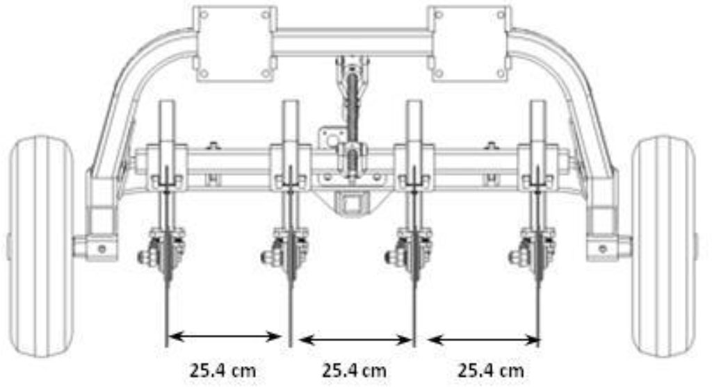
Figure 1 GCR sensor Veris Quad EC 1000 (VERIS-EC; 36).

FIGURE 2

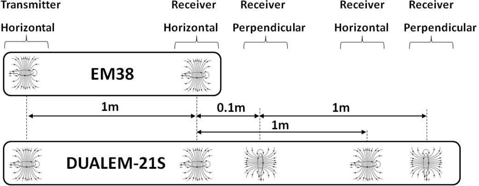
Figure 2 EMI sensors at normal position: EM-38 and DUALEM-21S, modified from Simpson et al. (22).

TABLE 1

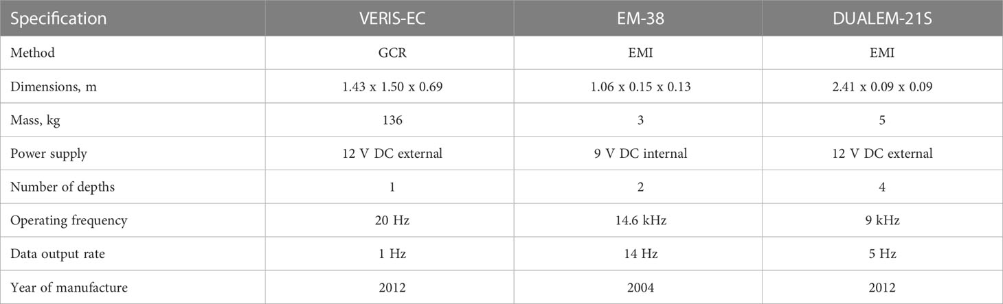
Table 1 Instrument specifications.

The VERIS-EC used in this study consisted of four rolling coulters and provided output related to shallow (0-30 cm) soil EC_a. The DUALEM-21S consisted of a 2.41 m long tube and had one transmitter coil and four receiving coils. Two of these four coils form a horizontal coplanar (HCP) array at 1 m (DUALEM_HCP-1) and 2 m (DUALEM_HCP-2) distances whereas the other two form a perpendicular coplanar (PRP) array at 1.1 m (DUALEM_PRP-1.1) and 2.1 m (DUALEM_PRP-2.1) distances. The sensing depths for all configurations can be found in Table 2. Finally, the EM-38 had only one pair of coplanar coils 1 m apart. The unit can be positioned in a horizontal dipole or a vertical dipole mode producing EC_a measurements related to 0.75 and 1.55 m deep soil profiles, respectively. This unit was calibrated before each use according to the manufacturer’s recommendations. Since the vertical dipole is the same as HCP, EM–38_HCP-1 and DUALEM_HCP-1 measurements are comparable (21), the EM-38 instrument was tested only in the vertical dipole configuration. All instruments went through the warming up period for about 5 minutes before each test event.

TABLE 2

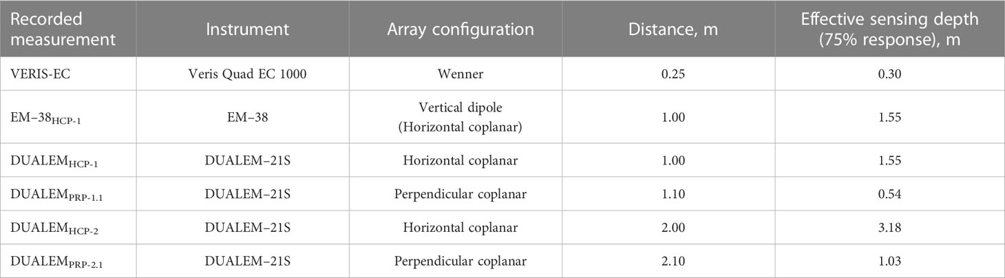
Table 2 List of recorded measurements.

A LabView (National Instruments, Corp., Austin, Texas, USA) application has been developed to automatically log data from the three sensors at individual data rates. A Watch Dog 2700 weather station (Spectrum Technologies, Inc., Aurora, Illinois, USA) was used to record ambient conditions that might affect instrument performances. Monitored ambient parameters were logged with a 5-min interval and included: air temperature and humidity, wind speed and direction, and rainfall. The same station was used to monitor soil temperature and water content 30 cm below the surface using an installed SMEC 300 (Spectrum Technologies, Inc., Aurora, Illinois, USA) stationary probe.

2.2 Experimental procedure

The instruments were placed in stationary positions approximately 8 m apart and about 6 m away from the data logging station, as shown in Figure 3. The setup distance was used to prevent signal distortion and interference with sensor readings. The test area at Macdonald Farm of McGill University, Quebec, Canada, was a regularly cut lawn approximately 2 m from the edge of a corn field. The soil type at the test location was identified as Chicot series, sandy loam with moderate water holding capacity, and moderate to poor drainage (37) and had relatively low soil EC_a.

FIGURE 3

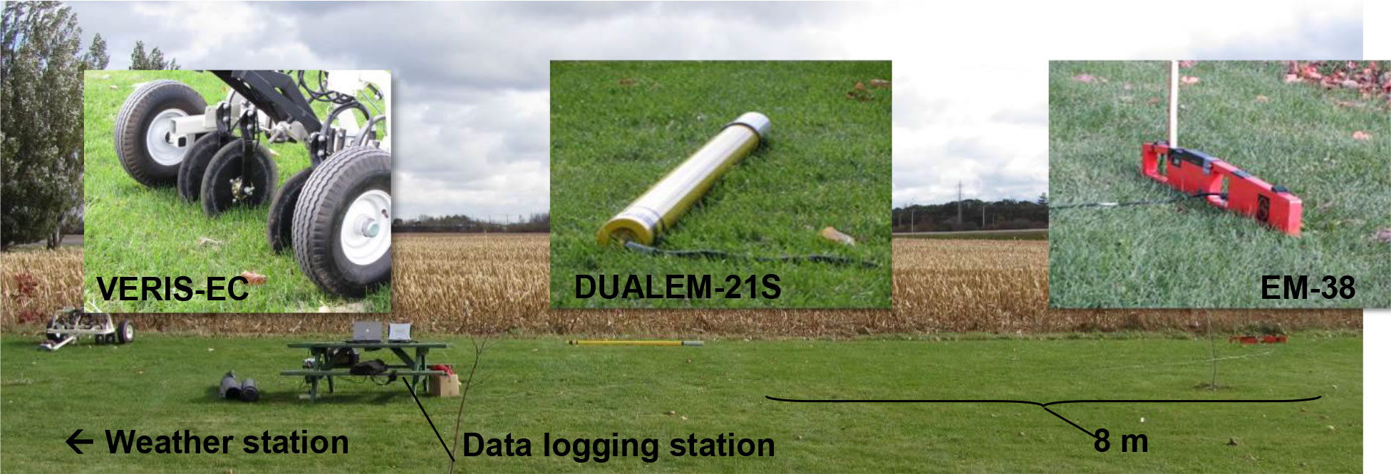
Figure 3 Experimental setup of CGR and EMI sensors (24-Oct).

A series of five 4.5-h data recordings were conducted from August to October. Each time, the instruments were placed in the same marked locations. The GCR coulter disks were pushed down gently (about 5 – 10 cm deep) to ensure good contact with the soil. At the same time, the EMI instruments were placed on the flat ground with the roll and pitch of the instruments as close to 0° (normal position) as possible. Another set of 5-min data recordings was conducted over several days from September to November with artificially introduced operational noise. Evaluated factors included: a) 10 cm height above the ground simulating an inconsistent distance between the instrument and soil surface, b) +10° and -10° pitch simulating potential raising of one end of the instrument, and c) +10° and -10° roll simulating deviation of the instrument from its vertical orientation (Figure 4) during a typical mapping exercise. The 0 cm height with 0° roll or pitch represents the typical normal position of the EMI sensors when placed on the ground during the mapping operation. The Table 3 summarizes all data acquisition events that allowed five replicates of temporal and three replicates of operational tests for every instrument.

FIGURE 4

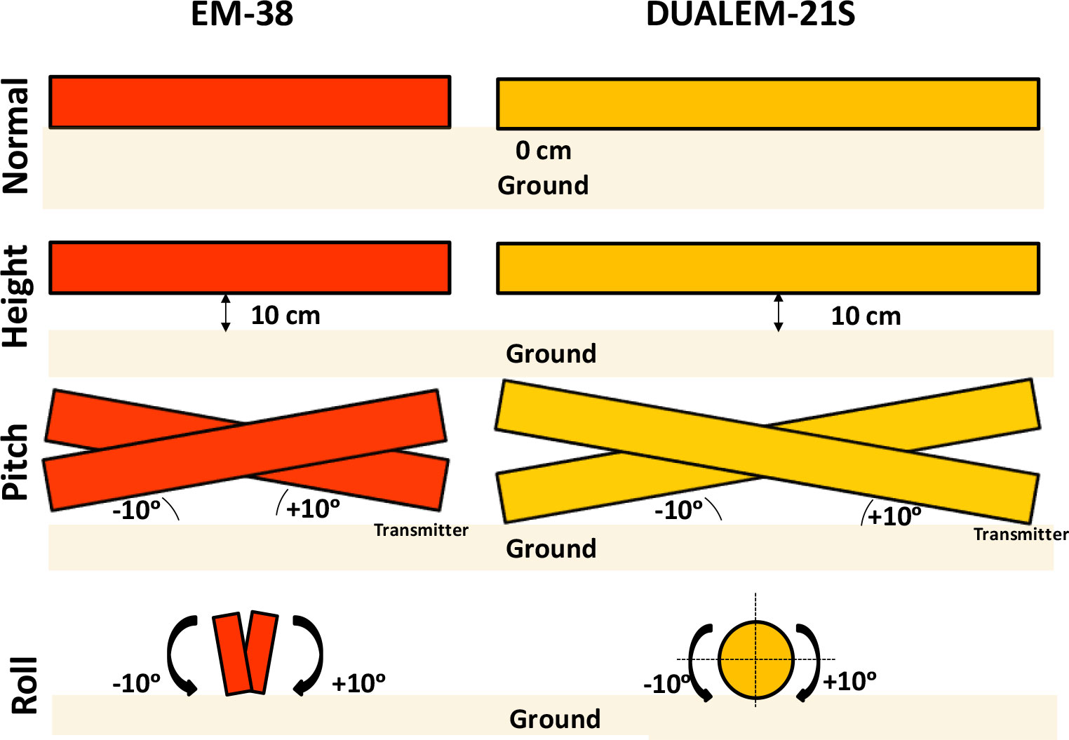
Figure 4 Operational tests for EMI instruments.

TABLE 3

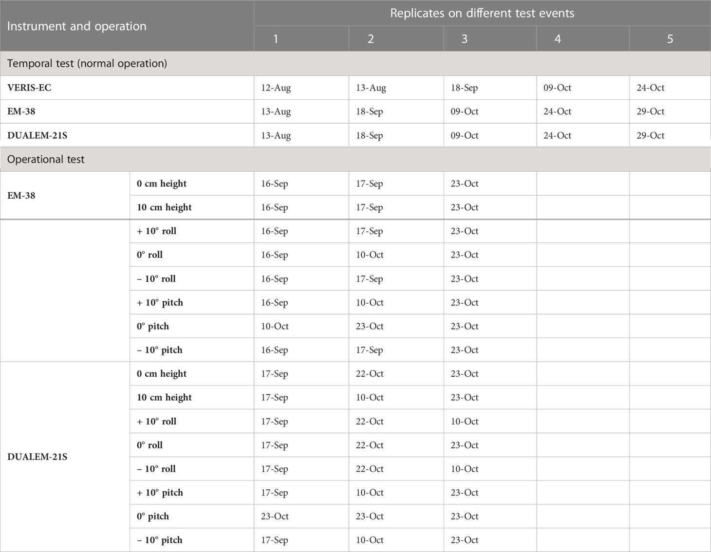
Table 3 Experimental timeline of CGR and EMI sensors for temporal and operational induced tests.

2.3 Data analysis

Data analysis was based on a comparison of 1-s data obtained at the highest possible rate without any filtering. While the temporal tests quantify the potential data drift from the beginning to the end of a single mapping exercise, the operational tests reveal the influence of typical uncertainties of the position of the instrument with respect to the ground. In addition, the test replicates show the influence of ambient conditions along with the possible uncertainties of sensor repositioning and other feasible inconstancies between test replicates.

For both temporal and operational tests, descriptive statistics, such as mean and standard deviation (STD) of each test replicate, were calculated. Root mean square errors (RMSE) for the temporal tests were estimated using the following equation:

$\begin{array}{ll}RMSE=\sqrt{\frac{1}{m(n-1)}{\displaystyle \sum _{i=1}^m{\displaystyle \sum _{j=1}^n{(\overline{E{C}_{ai}}-E{C}_{aij})}^2}}}& (1)\end{array}$

where n is the number of 1-s measurement averaged within any specific data log e.g. for 4.5 h; m is the number of different logging events of the test replicates e.g. 5 replications.

The Levene’s test of equal variances (e.g. 38) was conducted to compare mean square error (MSE) values corresponding to different instruments using the raw dataset. Due to a very large number of data records, high degrees of freedom made relatively similar variance estimates significantly different from each other. Therefore, a subjective grouping of similar RSME estimates was performed to facilitate the discussion. Thus, RMSE values less than 0.01 mS/m will be considered temporarily the most stable measurements, 0.01-0.50 mS/m as temporarily relatively stable measurements, and 0.5 mS/m or more as temporarily relatively unstable measurements. A simple linear regression was applied to the relationships between EC_a measurements and ambient conditions, including soil and air temperature, soil water content, air humidity, and internal temperature of the DUALEM-21S instrument. In terms of the operational test, a t–test using α = 0.05 was used to compare the means of three operational test replicates to the mean of nine replicates representing normal operation of the instrument (i.e., zero height, roll and pitch).

3 Results and discussions

3.1 Temporal test

Figure 5 indicates the range of air and soil temperatures, relative humidity, soil water content, and recorded internal instrument temperature of the DUALEM–21S during each 4.5-h temporal test. These tests generally cover all reasonable operational conditions when soil EC_a data are normally collected. The weather data captured from the weather station showed ambient and soil temperatures varying from 23.3 °C to freezing (-0.1 °C) and 29.5 to 7.6 °C, respectively. The latter measurements slightly vary within the same measurement date; however, they change greatly from one test event to another. The internal temperature of the DUALEM-21S ranged from 6 to 40 °C across the test dates. Assuming the ambient temperature effect is similar on all instruments, this temperature data then was used as a basis for the comparison between all these three instruments. The increase in soil moisture on 9-Oct was due to rainfall events during the two days prior to the test (6 mm of total precipitation).

FIGURE 5

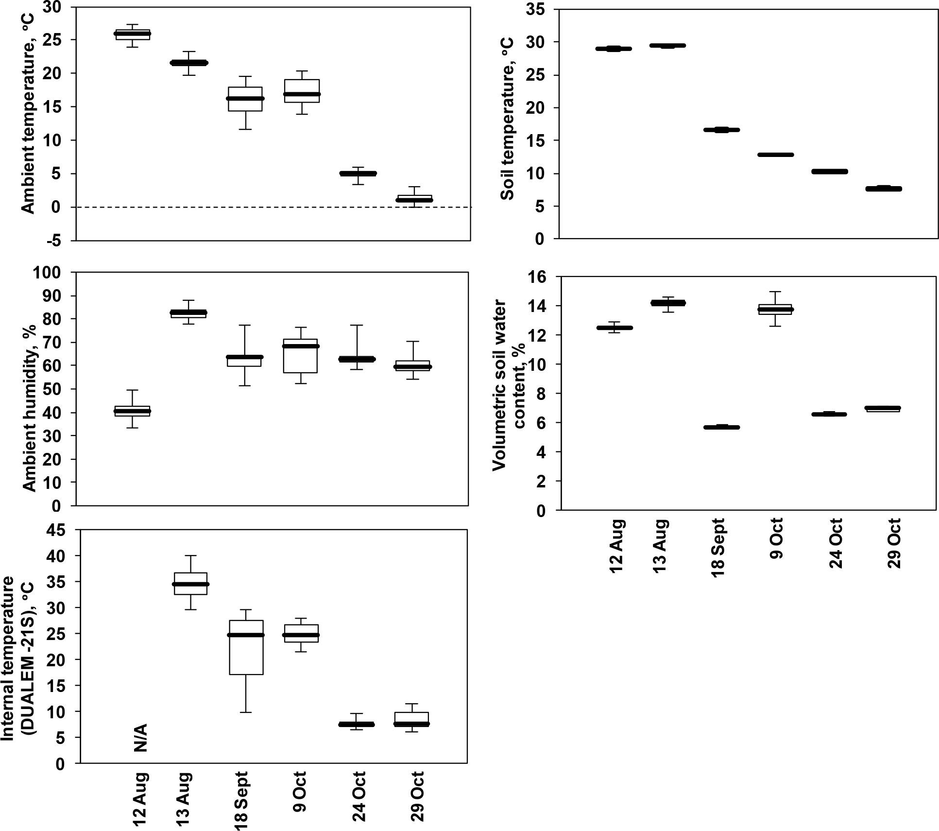
Figure 5 Box-and-whisker plots of environmental conditions: ambient temperature, soil temperature, air humidity, volumetric soil water content, and the internal temperature of DUALEM-21S instrument during temporal tests.

Figure 6 illustrates data logs for four different measurements obtained during the 9-Oct test. The ranges (minimum and maximum) for unprocessed soil EC_a measurements for the entire temporal test are presented in Figure 7. Table 4 summarizes the average, STD, and RMSE (Equation 1) values. The most stable soil EC_a measurements were from the GCR instrument. Earlier, Serrano et al. (33) observed a similar level of consistency of CGR measurements. Both DUALEM PRP measurements produced RMSE values 5-10 times smaller than those from the EM-38 or DUALEM HCP measurements. In addition to the 4.5-h drift of EC_a measurements, there were noticeable changes from day to day. For an unknown reason, the most apparent reduction in EC_a measurements was on 18-Sep for both DUALEM HCP measurements, but not for PRP. That day, the initial internal and ambient temperatures were similar (10.4 and 11.6°C), but a steady increase of the ambient temperature with relatively low wind speed (around 2 km/h) may have resulted in rapid solar warming of the instrument. This typically reduces soil EC_a measurements. However, it is not certain what caused this sensor behaviour.

FIGURE 6

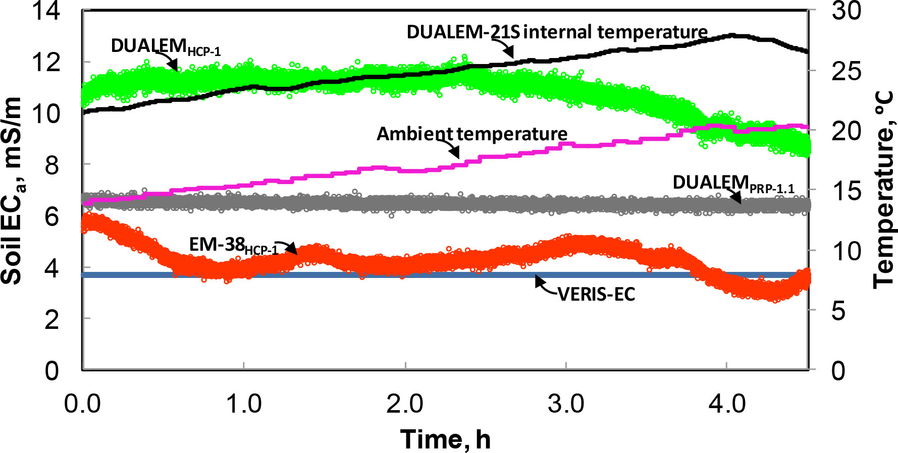
Figure 6 An example of 1-s soil EC_a measurement logs obtained on 9-Oct.

FIGURE 7

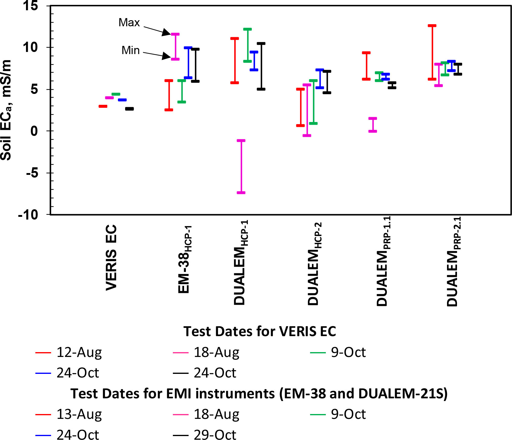
Figure 7 The range (minimum and maximum) of soil EC_a measurements during temporal tests.

TABLE 4

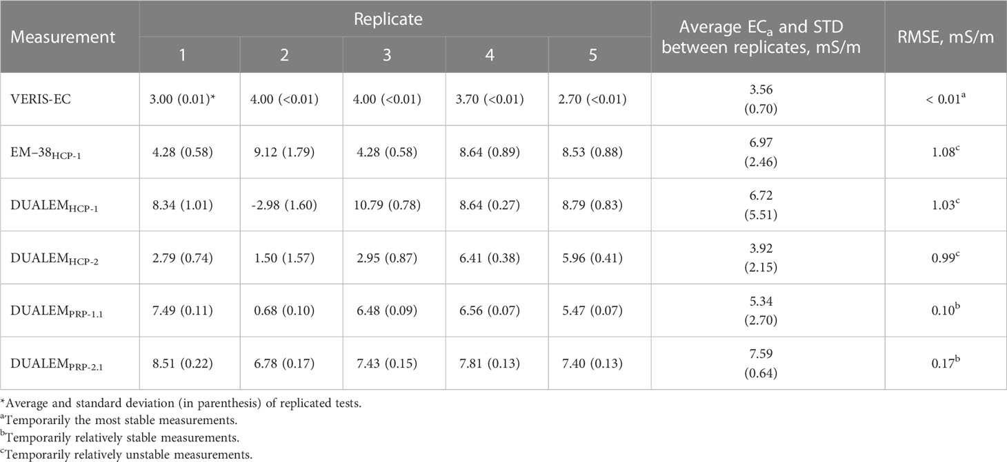
Table 4 EC_a (mS/m) measurements for temporal tests.

Table 5 summarizes the correlation coefficients for a linear regression between ambient conditions and recorded measurements. Figure 8 demonstrates the relationships between air, soil and internal DUALEM instrument temperatures with several EC_a measurements. It is obvious that an anomaly, such as the 18-Sep drop in DUALEM HCP measurements, affected the observed relationships. This anomaly cannot be explained by ambient conditions and may be affiliated with a number of unaccounted for factors, such as instrument positioning and the conditions of surrounding vegetation. When disregarded, it appears that the EM-38 measurements are negatively correlated with ambient and internal temperatures. According to Allred et al. (19), low soil water content and high temperature normally reduces soil EC_a. Sudduth et al. (18) reported that the drift over 10% of EC_a observed during field mapping using the EM-38 might be due to a change in internal temperature rather than ambient temperature variations. Corwin and Lesch (11) recommend converting EC_a measurements at a specific temperature to measurements at a reference temperature (e.g., 25°C). Naturally, this would mean that temperature-compensated VERIS-EC and DUALEM-21S measurements would not be affected by ambient conditions to the extent of non-compensated EM-38 measurements. However, the presented data have not revealed temperature-induced changes in EM-38 measurements greater than other effects, such as instrument repositioning. The effects of soil temperature and water content are less quantifiable since they did not change significantly during individual tests.

TABLE 5

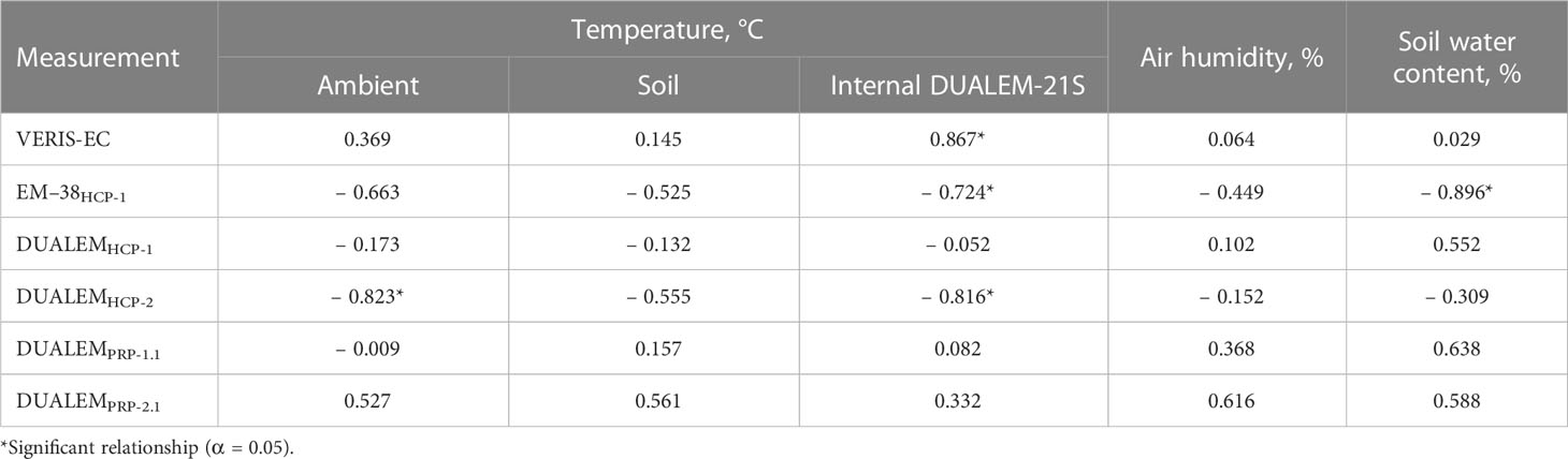
Table 5 Pearson coefficients of correlation between EC_a measurements and measurement conditions.

FIGURE 8

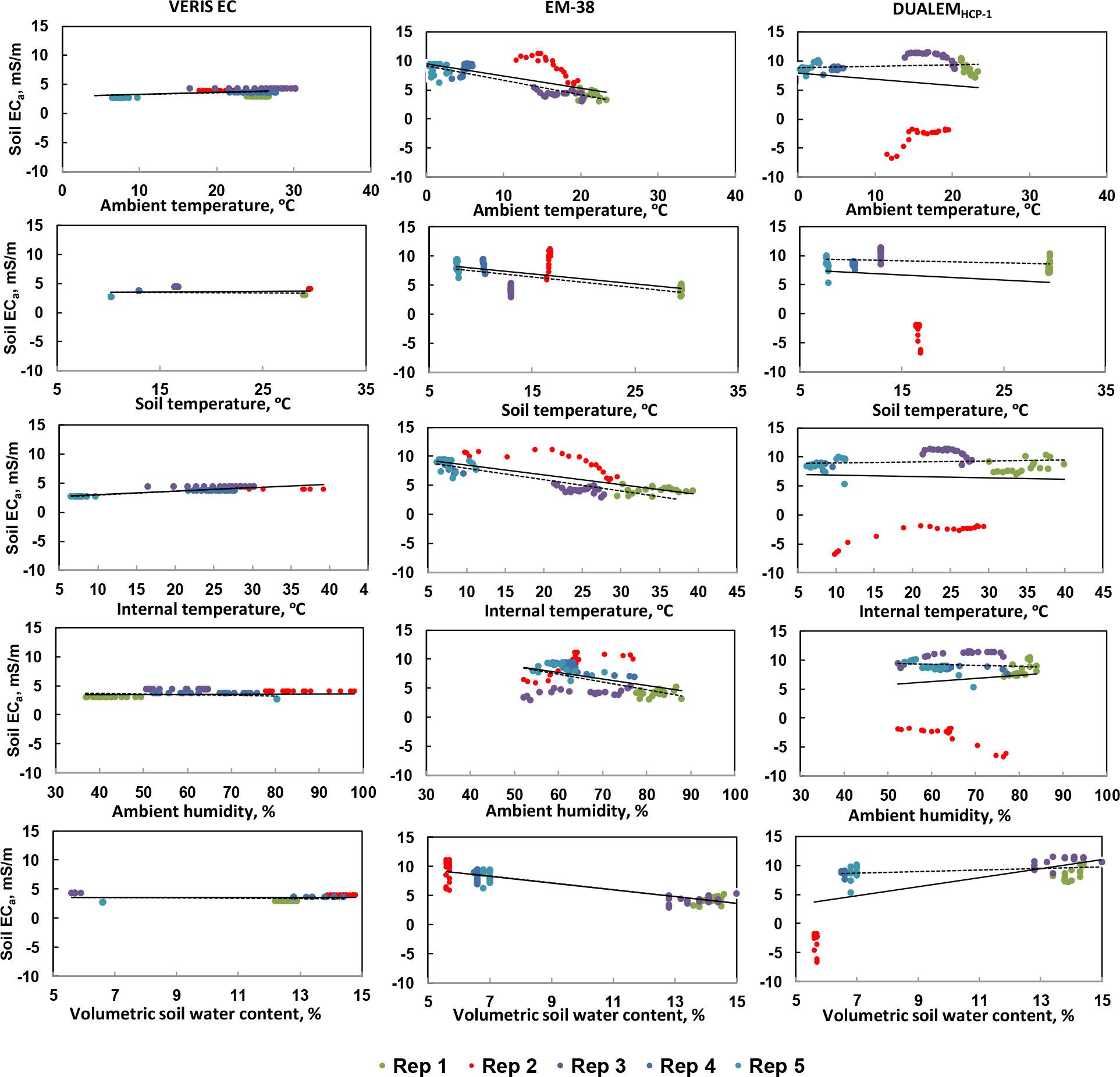
Figure 8 Examples of relationships between EC_a measurements (15-min sampling) and corresponding records of ambient conditions (dash lines show regressions with 18-Sep data excluded). Rep 1 through Rep 5 represents the test replication on different test events.

3.2 Operational test

Figure 9 provides the results of the operational tests (minimum and maximum values) for both EMI sensors for height (0 and 10 cm), roll (−10°, 0°, +10°) and pitch (−10°, 0°, +10°) tests. Each 5-min data log represented a particular test configuration that was repeated in random order on three different occasions during at least two different days. Since normal operation (zero height, pitch and roll) was part of each operational test, this configuration has been replicated nine times. Table 6 shows the individual soil EC_a test average, STD and t-test p-values. In this case, the average of three operational test replicate means were compared with the average of nine normal operation means.

FIGURE 9

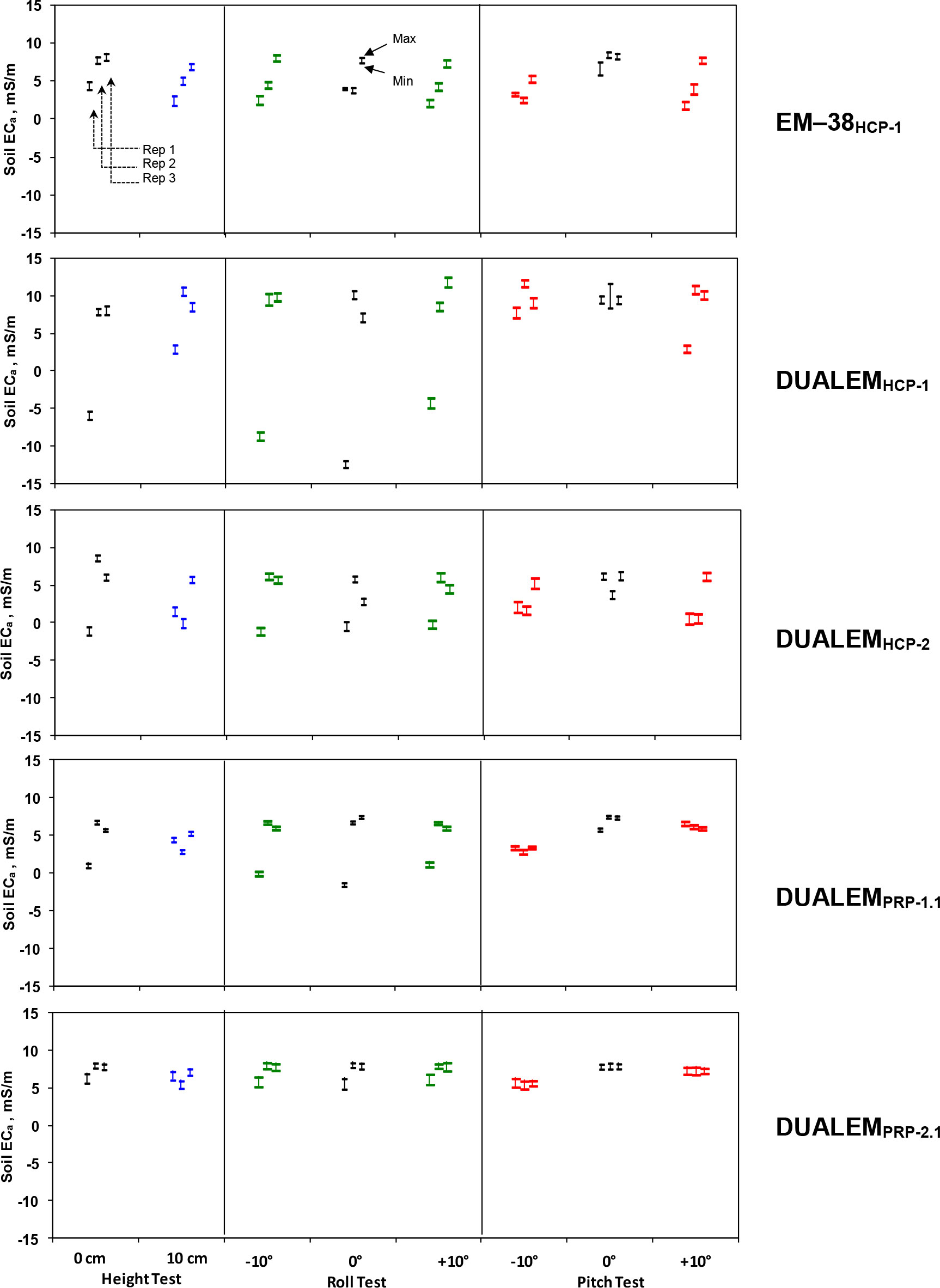
Figure 9 The range (minimum and maximum) of operational tests for each recorded measurement. Rep 1 through Rep 3 represents the test replication on different test events. Different colors represent different operation tests in relative to the normal position of 0°.

TABLE 6

Table 6 (The soil EC_a (mS/m) measurements for operational tests.

It appears that raising the instrument did not contribute to greater EC_a measurement changes than the differences between replicates. In most cases, HCP measurements decrease when the instrument is raised in the air, but this may not be the case for some sensor configuraions if high EC_a soil overlays less conductive subsoil. A marginal significance of the drop in average EC_a caused by the raised instrument was found for DUALEM_PRP-2.1 which may have been due to the relatively low EC_a difference between replicates rather than the magnitude of this change. In terms of the pitch and roll tests, it appears that the 10° deviations from the normal operation did not have a significant effect on the recorded measurements. The exceptions were EM-38_HCP-1 and DUALEM_PRP-2.1 when the end of the instrument containing the transmitting coil was raised above the ground.

From a practical standpoint, the results of this study indicate that GCR sensing of EC_a may be less sensitive to temporal effects than EMI measurements in many situations and may have be appealing for many environments test. However, the non-contact nature of EMI measurements provides versatility with respect to the measurement environment and, when designing the deployment platform, such as sled (32, 39), these instruments should stay close to the ground with zero pitch and roll. It was determined to be very important to keep the transmitting coil close to the ground. Minor deviations from these conditions do not affect measurements to a greater degree than temporal test replications.

4 Conclusion

A set of stationary tests of one GCR and two EMI instruments revealed the degree of temporal and operation-induced variations on observed measurements of EC_a. While the GCR instrument was relatively immune to long-term data drifts, repositioning the EMI instruments on the soil surface at different times of the year (different soil conditions and ambient temperatures) provided more noticeable differences. Furthermore, EMI measurements were less stable during 4.5-h log periods than the CGR instrument. Also, it was noted that the PRP configuration was more stable over time than the HCP operation. The same applies to the operational tests. The effects of instrument height, roll and pitch were smaller than the differences from test event to test event, which could be attributed to a number of uncontrolled factors, including exact position of the instrument and different environmental parameters. However, practitioners should avoid, or minimize, raising the transmitting coil end of the instrument due to the reported sensitivity of EC_a measurements to this experimental treatment.

Data availability statement

The original contributions presented in the study are included in the article/supplementary materials, further inquiries can be directed to the corresponding author/s.

Author contributions

AMS and VA conceptualized and designed the study, AMS collected the data, analyzed the data and drafted the manuscript, VA reviewed, and edited the manuscript. All authors contributed to the article and approved the submitted version.

Funding

This project was funded in part by Canada Foundation for Innovation (CFI) Leader Opportunity Fund (LOF), Ministry of Higher Education Malaysia (MOHE) and Universiti Putra Malaysia (UPM).

Conflict of interest

The authors declare that the research was conducted in the absence of any commercial or financial relationships that could be construed as a potential conflict of interest.

Publisher’s note

All claims expressed in this article are solely those of the authors and do not necessarily represent those of their affiliated organizations, or those of the publisher, the editors and the reviewers. Any product that may be evaluated in this article, or claim that may be made by its manufacturer, is not guaranteed or endorsed by the publisher.

References

1. De Jong E, Ballantyne A, Cameron D, Read D. Measurement of apparent electrical conductivity of soils by an electromagnetic induction probe to aid salinity surveys. Soil Sci Soc America J (1979) 43:810–2. doi: 10.2136/sssaj1979.03615995004300040040x

CrossRef Full Text | Google Scholar

2. Williams BG, Hoey D. The use of electromagnetic induction to detect the spatial variability of the salt and clay contents of soils. Soil Res (1987) 25:21–7. doi: 10.1071/SR9870021

CrossRef Full Text | Google Scholar

3. Lesch SM, Strauss DJ, Rhoades JD. Spatial prediction of soil salinity using electromagnetic induction techniques: 1. statistical prediction models: a comparison of multiple linear regression and cokriging. Water Resour Res (1995) 31:373–86. doi: 10.1029/94WR02179

CrossRef Full Text | Google Scholar

4. Amidu SA, Dunbar JA. An evaluation of the electrical-resistivity method for water-reservoir salinity studies. Geophysics (2008) 73:G39–49. doi: 10.1190/1.2938994

CrossRef Full Text | Google Scholar

5. Slavich P, Petterson G. Estimating the electrical conductivity of saturated paste extracts from 1: 5 soil, water suspensions and texture. Soil Res (1993) 31:73–81. doi: 10.1071/SR9930073

CrossRef Full Text | Google Scholar

6. Corwin DL, Lesch SM. Application of soil electrical conductivity to precision agriculture: theory, principles, and guidelines. Agron J (2003) 95:455–71. doi: 10.2134/agronj2003.4550

CrossRef Full Text | Google Scholar

7. Tetegan M, Pasquier C, Besson A, Nicoullaud B, Bouthier A, Bourennane H, et al. Field-scale estimation of the volume percentage of rock fragments in stony soils by electrical resistivity. Catena (2012) 92:67–74. doi: 10.1016/j.catena.2011.09.005

CrossRef Full Text | Google Scholar

8. Kachanoski R, Wesenbeeck IV, Gregorick E. Estimating spatial variations of soil water content using noncontacting electromagnetic inductive methods. Can J Soil Sci (1988) 68:715–22. doi: 10.4141/cjss88-069

CrossRef Full Text | Google Scholar

9. Sheets KR, Hendrickx JMH. Noninvasive soil water content measurement using electromagnetic induction. Water Resour Res (1995) 31:2401–9. doi: 10.1029/95WR01949

CrossRef Full Text | Google Scholar

10. Michot D, Benderitter Y, Dorigny A, Nicoullaud B, King D, Tabbagh A. Spatial and temporal monitoring of soil water content with an irrigated corn crop cover using surface electrical resistivity tomography. Water Resour Res (2003) 39:1138. doi: 10.1029/2002WR001581

CrossRef Full Text | Google Scholar

11. Corwin DL, Lesch SM. Apparent soil electrical conductivity measurements in agriculture. Comput Electron Agric (2005) 46:11–43. doi: 10.1016/j.compag.2004.10.005

CrossRef Full Text | Google Scholar

12. Brevik EC, Fenton TE, Lazari A. Soil electrical conductivity as a function of soil water content and implications for soil mapping. Precis Agric (2006) 7:393–404. doi: 10.1007/s11119-006-9021-x

CrossRef Full Text | Google Scholar

13. Brillante L, Bois B, Mathieu O, Bichet V, Michot D, Lévêque J. Monitoring soil volume wetness in heterogeneous soils by electrical resistivity. A field-based pedotransfer function. J Hydrology (2014) 516:56–66. doi: 10.1016/j.jhydrol.2014.01.052

CrossRef Full Text | Google Scholar

14. Paillet Y, Cassagne N, Brun J-J. Monitoring forest soil properties with electrical resistivity. Biol Fertil Soils (2010) 46:451–60. doi: 10.1007/s00374-010-0453-0

CrossRef Full Text | Google Scholar

15. Allred B, Daniels JJ, Ehsani MR. Handbook of agricultural geophysics. CRC Press (2008).

Google Scholar

16. Parasnis DS. Principles of applied geophysics. 5th ed. London, UK: Chapman & Hall (1997). p. 456.

Google Scholar

17. Pan L, Adamchuk V, Prasher S, Gebbers R, Taylor R, Dabas M. Vertical soil profiling using a galvanic contact resistivity scanning approach. Sensors (2014) 14:13243–55. doi: 10.3390/s140713243

PubMed Abstract | CrossRef Full Text | Google Scholar

18. Sudduth KA, Drummond ST, Kitchen NR. Accuracy issues in electromagnetic induction sensing of soil electrical conductivity for precision agriculture. Comput Electron Agric (2001) 31:239–64. doi: 10.1016/S0168-1699(00)00185-X

CrossRef Full Text | Google Scholar

19. Allred B, Ehsani MR, Saraswat D. Comparison of electromagnetic induction, capacitively-coupled resistivity, and galvanic contact resistivity methods for soil electrical conductivity measurement. Appl Eng Agric (2006) 22:215–30. doi: 10.13031/2013.20283

CrossRef Full Text | Google Scholar

20. Abdu H, Robinson D, Jones SB. Comparing bulk soil electrical conductivity determination using the DUALEM-1S and EM38-DD electromagnetic induction instruments. Soil Sci Soc America J (2007) 71:189–96. doi: 10.2136/sssaj2005.0394

CrossRef Full Text | Google Scholar

21. Saey T, Simpson D, Vermeersch H, Cockx L, Van Meirvenne M. Comparing the EM38DD and DUALEM-21S sensors for depth-to-clay mapping. Soil Sci Soc America J (2009) 73:7–12. doi: 10.2136/sssaj2008.0079

CrossRef Full Text | Google Scholar

22. Simpson D, Van Meirvenne M, Saey T, Vermeersch H, Bourgeois J, Lehouck A, et al. Evaluating the multiple coil configurations of the EM38DD and DUALEM-21S sensors to detect archaeological anomalies. Archaeological Prospection (2009) 16:91–102. doi: 10.1002/arp.349

CrossRef Full Text | Google Scholar

23. Sudduth KA, Kitchen NR, Myers DB, Drummond ST. Mapping depth to argillic soil horizons using apparent electrical conductivity. J Environ Eng Geophysics (2010) 15:135–46. doi: 10.2113/JEEG15.3.135

CrossRef Full Text | Google Scholar

24. Urdanoz V, Aragüés R. Comparison of geonics EM38 and dualem 1S electromagnetic induction sensors for the measurement of salinity and other soil properties. Soil Use Manage (2012) 28:108–12. doi: 10.1111/j.1475-2743.2011.00386.x

CrossRef Full Text | Google Scholar

25. Robinson DA, Lebron I, Lesch SM, Shouse P. Minimizing drift in electrical conductivity measurements in high temperature environments using the EM-38. Soil Sci Soc America J (2004) 68:339–45. doi: 10.2136/sssaj2004.3390

CrossRef Full Text | Google Scholar

26. Allred B, Ehsani M, Saraswat D. The impact of temperature and shallow hydrologic conditions on the magnitude and spatial pattern consistency of electromagnetic induction measured soil electrical conductivity. Trans ASAE (2005) 48:2123–35. doi: 10.13031/2013.20098

CrossRef Full Text | Google Scholar

27. Taylor R, Holladay J. Accurate electromagnetic measurement of apparent conductivity: issues and applications. In 3rd Global Workshop on Proximal Soil Sensing (2013) 2013:62.

Google Scholar

28. Brevik E, Fenton T, Horton R. Effect of daily soil temperature fluctuations on soil electrical conductivity as measured with the geonics® EM-38. Precis Agric (2004) 5:145–52. doi: 10.1023/B:PRAG.0000022359.79184.92

CrossRef Full Text | Google Scholar

29. Farahani H, Buchleiter G. Temporal stability of soil electrical conductivity in irrigated sandy fields in Colorado. Trans ASAE (2004) 47:79–90. doi: 10.13031/2013.15873

CrossRef Full Text | Google Scholar

30. Doolittle J, Sudduth K, Kitchen N, Indorante S. Estimating depths to claypans using electromagnetic induction methods. J Soil Water Conserv (1994) 49:572–5.

Google Scholar

31. Roy A. Depth of investigation in wenner, three-electrode and dipole-dipole DC resistivity methods. Geophysical Prospecting (1972) 20:329–40. doi: 10.1111/j.1365-2478.1972.tb00637.x

CrossRef Full Text | Google Scholar

32. Adamchuk V, Su AM, Eigenberg RA, Ferguson RB. Development of an angular scanning system for sensing vertical profiles of soil electrical conductivity. Trans ASABE (2011) 54(3):757–67. doi: 10.13031/2013.37091

CrossRef Full Text | Google Scholar

33. Serrano J, Shahidian S, Silva J. Spatial and temporal patterns of apparent electrical conductivity: DUALEM vs. veris sensors for monitoring soil properties. Sensors (2014) 14:10024–41. doi: 10.3390/s140610024

PubMed Abstract | CrossRef Full Text | Google Scholar

34. Brevik E, Fenton T, Lazari A. Differences in EM-38 readings taken above crop residues versus readings taken with instrument-ground contact. Precis Agric (2003) 4:351–8. doi: 10.1023/A:1026319307801

CrossRef Full Text | Google Scholar

35. de Assis Silva S, dos Santos RO, de Queiroz DM, de Souza Lima JS, Pajehú LF, Medauar CC. Apparent soil electrical conductivity in the delineation of management zones for cocoa cultivation. Inf Process Agric (2022) 9(3):443–55. doi: 10.1016/j.inpa.2021.04.004

CrossRef Full Text | Google Scholar

36. Veris Technologies, Inc. (2014). Available at: http://www.veristech.com/the-soil/soil-ec (Accessed 17 November 2014).

Google Scholar

37. Lajoie PG. Soil survey of argenteuil, two mountains and terrebonne counties, Quebec (1960). Research Blanch, Canada Department of Agriculture in co-operation with Quebec Department of Agriculture and Macdonald College, McGill University. Available at: http://sis.agr.gc.ca/cansis/publications/surveys/pq/pq2/index.html (Accessed 8 November 2014).

Google Scholar

38. National Institute of Standards and Technology (NIST). U.S. department of commerce (2022). Available at: https://www.itl.nist.gov/div898/handbook/eda/section3/eda35a.htm (Accessed 31st December 2022).

Google Scholar

39. Peralta NR, Alesso CA, Costa JL, Martin NF. Mapping soil depth in southern pampas Argentina using ancillary data and statistical learning. Soil Sci Soc America J (2022) 86(1):65–78. doi: 10.1002/saj2.20350

CrossRef Full Text | Google Scholar