 Ricardo Canal Filho
 José Paulo Molin
95% of researchers rate our articles as excellent or good
Learn more about the work of our research integrity team to safeguard the quality of each article we publish.
Find out more
ORIGINAL RESEARCH article
Front. Soil Sci. , 03 October 2022
Sec. Soil Management
Volume 2 - 2022 | https://doi.org/10.3389/fsoil.2022.984963
In soil science, near-infrared (NIR) spectra are being largely tested to acquire data directly in the field. Machine learning (ML) models using these spectra can be calibrated, adding only samples from one field or gathering different areas to augment the data inserted and enhance the models’ accuracy. Robustness assessment of prediction models usually rely on statistical metrics. However, how the spatial distribution of predicted soil attributes can be affected is still little explored, despite the fact that agriculture productive decisions depend on the spatial variability of these attributes. The objective of this study was to use online NIR spectra to predict soil attributes at field level, evaluating the statistical metrics and also the spatial distribution observed in prediction to compare a local prediction model with models that gathered samples from other areas. A total of 383 online NIR spectra were acquired in an experimental field to predict clay, sand, organic matter (OM), cation exchange capacity (CEC), potassium (K), calcium (Ca), and magnesium (Mg). To build ML calibrations, 72 soil spectra from the experimental field (local dataset) were gathered, with 59 samples from another area nearby, in the same geological region (geological dataset) and with this area nearby and more 60 samples from another area in a different region (global dataset). Principal components regression was performed using k-fold (k=10) cross-validation. Clay models reported similar errors of prediction, and although the local model presented a lower R2 (0.17), the spatial distribution of prediction proved that the models had similar performance. Although OM patterns were comparable between the three datasets, local prediction, with the lower R2 (0.75), was the best fitted. However, for secondary NIR response attributes, only CEC could be successfully predicted and only using local dataset, since the statistical metrics were compatible, but the geological and global models misrepresented the spatial patterns in the field. Agronomic plausibility of spatial distribution proved to be a key factor for the evaluation of soil attributes prediction at field level. Results suggest that local calibrations are the best recommendation for diffuse reflectance spectroscopy NIR prediction of soil attributes and that statistical metrics alone can mispresent the accuracy of prediction.
Proximal soil sensing (PSS) is a relevant technique to make soil data acquisition faster and more cost effective (1, 2). In this sense, many authors have studied techniques to be adapted for PSS. Diffuse reflectance spectroscopy (DRS) in the visible (Vis) and near-infrared region (NIR) has been largely tested to predict soil physical and chemical attributes (3, 4). The prediction can perform on primary NIR response attributes, which means attributes like clay and organic matter (OM), that have direct spectral absorption patterns in this region or even on secondary response attributes that do not have direct patterns in NIR but can be predicted due to the construction of indirect calibrations.
The idea of using machine learning (ML) models of DRS NIR spectra for soil attributes prediction lies into the choice of the statistical model and then in the accurate prediction of these attributes. Dimensionality reduction models are often chosen due to the multidimensionality of soil spectra (5). Besides coping with multivariate data analysis (6), dimensionality reduction models can sometimes smooth the values predicted, loosing extreme values that the model considers as outliers (7) and therefore needs careful implementation. In this sense, principal components regression (PCR) is a multivariate method of simple implementation, which had its potential demonstrated since the beginning of studies for soil properties prediction using DRS. Authors reported successful prediction of this technique for diverse soil attributes, such as soil organic carbon, organic matter, pH, and macronutrients, such as total nitrogen and total and extractable phosphorus and potassium (8–12). Then, statistical metrics are being used for the assessment of ML model robustness (13), such as the coefficient of determination (R2), which gives the idea of the variance portion of the data that the model is explaining; the root mean squared error (RMSE) and mean absolute error (MAE), which represent the error of prediction the model offered; and the ratio of performance to interquartile distance (RPIQ), which is calculated using the RMSE and the range between first and third quantiles of the data.
However, precision agriculture (PA) has in its very definition the consideration of temporal and spatial variability of agricultural production (14). This fact comes from the necessity of understanding the patterns of the variability in the field, since agriculture needs to adapt or act in the variability of production. Soil physical and chemical attributes have well-known relations and patterns defined by soil science in the study of agricultural soil fertility, and these relations are studied by means of the spatial dependence in geostatistics (15). The range of a fitted variogram means the distance in which a point is still related, or spatial dependent, to another.
With this knowledge, investigations show that the relation between soil attributes will affect the construction of ML models. Early when DRS were tested for PSS, Stenberg et al. (16) stated that prediction models using Vis-NIR spectrum should consider only samples from the same morphopedological formation, since the variations in soil mineralogy will affect the spectral signature, and the model will not be able to accurately predict attributes with this variation. Nevertheless, studies have been reaching satisfactory prediction metrics in constructing models not only with the fusion of samples from the same geological region (17, 18) but also using samples from fields with different soil formations (19).
The statistical metrics are important to define the accuracy of a prediction model. However, the way the ML calibration affects the distribution of attributes should be considered with the same importance, since this distribution will directly affect the decision making in agriculture productive process. Hence, this study aimed to understand if the insertion of outside samples in the calibration of NIR soil attributes prediction models affects the spatial dependence of predicted values. The objective was to define whether the spatial distribution should be always taken into account when evaluating the quality of prediction from an ML model for both primary and secondary NIR response soil attributes.
The steps followed for this study development are summarized by the flowchart shown in Figure 1. These steps will be further explained in details.
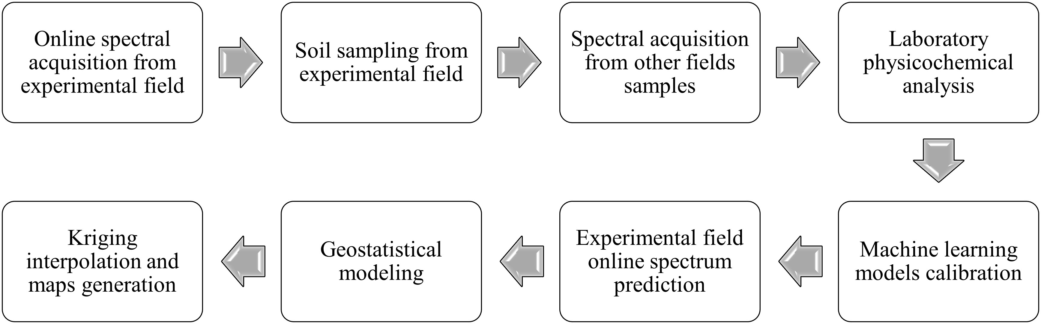
Figure 1 Flowchart of steps developed in this study.
The study area is located in Piracicaba, São Paulo state, Brazil (22°43'03.51"S, 47°36'50.03"W), where online NIR spectra were acquired for high spatial resolution prediction of soil attributes. Following the criteria of using another area from the same geological formation region, samples from another area of 3,300 m distance from the experimental field, described in Eitelwein (20), were used (22°41'57.64"S, 47°38'33.13"W). For the composition of a dataset with samples from multiple geological formations, samples were added from an area located in Mato Grosso state, Brazil (14°06'05.02"S, 57°46'01.66"W), also described in Eitelwein (20) (Figure 2).
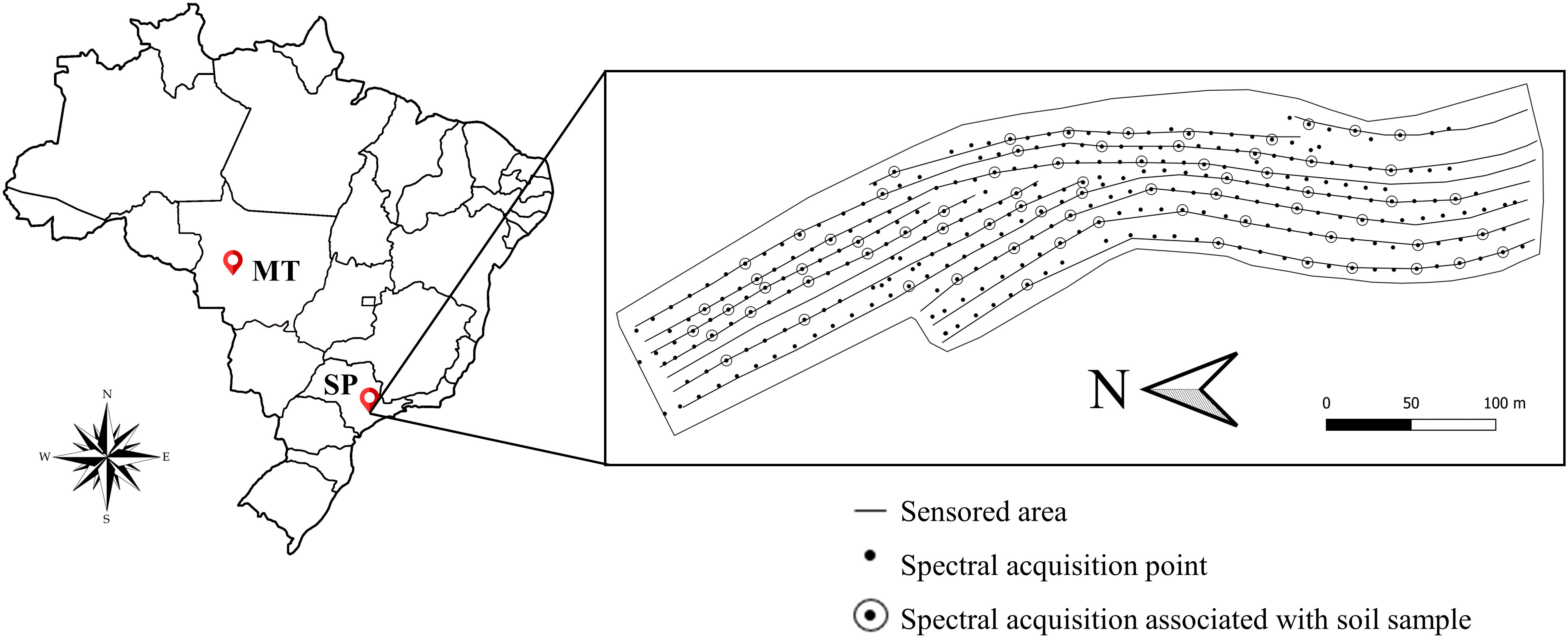
Figure 2 Location of areas from where samples were acquired for models’ calibrations. Highlighted, located in Piracicaba, São Paulo State (SP), the experimental field shape, sensored transects, spectral points acquisition, and associated soil samples. Samples from another field nearby were used to compose geological dataset. Global dataset was built by adding samples from another area, located in Mato Grosso (MT) state.
In November 2021, online soil spectral data were acquired using a structure mounted on the three-point hydraulic hitch of a tractor. A subsoiler shank was attached to this structure carrying a steel armored case that protects the NIR spectrophotometer (MicroNIR from VIAVI Solutions Inc., USA). The tip of the shank makes the 0.15-m-depth furrow, and the soil is smoothed by the bottom of the case, where the NIR spectrophotometer collects online soil spectra through a sapphire window at a spectral resolution of 908.1–1676.2 nm, every 6.2 nm, resulting in 125 different wavelengths. Spectra are collected at the base of the case, which were transported by a USB cable, converted for transmission via an ethernet cable, and recorded on a laptop computer. A 99% reflectance disk was used as reference for white (maximum reflectance), and the equipment itself has an internal reference measurement for black (minimum reflectance). Each spectrum collected in the field was associated with its geographic coordinates using a Global Navigation Satellite System (GNSS) Ag-Star (Novatel, Calgary, Canada) receiver with TerraStarC differential correction (Hexagon, Alabama, USA). The tractor traveled the area in the normal direction of the machine traffic, limited by the presence of terraces and with 12 m between each transect sensored. The spectrometer carries an internal data acquisition that groups spectra samples using principal components, excluding samples that are outside the confidence interval established in the software, and thus generates a spectrum by the mean. The acquisition time was 10 s each at a speed of 0.583 m s−1 (2.1 km h−1), resulting in 383 online NIR spectra acquired. During the field operation, 72 random starting sensing points (12 samples ha−1), indicated by the acquisition software, were demarcated and further sampled at the bottom of the furrow, excluding 1.0 m at the beginning and at the end of the transect, which aimed to overlap the area that corresponded to an online spectrum acquired (Figure 3). Those samples were submitted for laboratory analysis and used for model calibration. In addition, the density of 12 samples ha−1 allowed to generate maps from laboratory analysis to be used as counter proof of the models’ prediction.
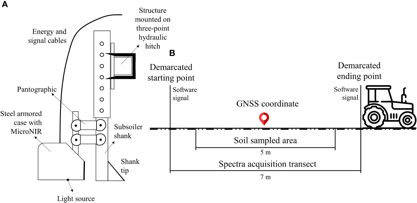
Figure 3 (A) Scheme of subsoiler shank carrying the spectrophotometer; (B) scheme of spectral acquisition, associated soil sample, and coordinate.
Soil physicochemical analysis were carried out on a commercial laboratory. The soil attributes that were considered and the respective analysis method were as follows: clay and sand, HMFS+NaOH; OM, oxidation; cation exchange capacity (CEC), sum of basis (resin) plus soil total acidity (KCl); and magnesium (Mg), potassium (K), and calcium (Ca), resin. Phosphorus models were discarded, as the preliminary analysis presented its independence distribution with primary NIR response attributes in the experimental area (7).
The software Jupyter Notebook (21, 22) was used for data processing. Calibration models were built using three datasets: local—only the 72 samples from the experimental field; geological—adding 59 samples from a field of the same morphopedological region, nearby; and global—adding 60 samples from a field in Mato Grosso on the geological dataset. Adding samples from other areas is a strategy adopted by researchers to augment the number of observations in the calibration, thus improving the accuracy of model (19, 23, 24).
The statistical model used was the principal components regression (PCR). PCR is a dimensionality reduction model, indicated to build calibrations with soil spectra due to its multidimensionality characteristic and the possible collinearity among variables (5). Velliangiri and Alagumuthukrishnan (6) described that dimensionality reduction models, such as PCR, can aid ML models in the removal of noisy and redundant data. Therefore, raw spectral data were used for models calibration in this study.
Each dataset was randomly divided in the proportion of 70% for calibration and 30% for validation, using k-fold (k = 10) cross-validation (25), which is recommended for the evaluation of ML models to reduce bias. A random state in the software function was always set to ensure repeatability and that after the split, the same 21 samples from the experimental field would be used for the validation of all three calibration strategies. The assessment of the models’ accuracy was performed using common metrics from the literature of soil attributes prediction using Vis-NIR spectra: R2, RMSE, MAE, and RPIQ. The parameters were evaluated and showed that the higher the R2 and RPIQ values and the lower the RMSE and the MAE values, the better is the model performance.
The models calibrated were then used to predict the soil attributes considered using the online spectra acquired in the experimental field. A descriptive analysis aiming to exclude acquisition points, like field borders, was carried out before the prediction, which resulted in the use of 303 online spectra for prediction that were then used for data interpolation. Data of each attribute were individually interpolated by ordinary kriging, using the software VESPER (26). The method used was block kriging, in 3.0 × 3.0 m pixels, and the minimum and maximum neighboring points for interpolation was determined as 4 and 300, respectively. Additional kriging parameters are available in Supplementary Material Table A1. After kriging interpolation, the maps generated for each predicted attribute were exported to QGIS software (27) for analysis and comparison.
The correlation observed among soil attributes can indicate that a secondary calibration can be explored (7). The Pearson correlations of datasets used in this study are presented in Figure 4. For the local dataset, which only contains samples from the experimental field, the only primary–secondary NIR response attributes correlation observed is OM-CEC of 0.76. On the other hand, the geological and global datasets presented all common physicochemical correlations: clay and OM strongly and positively correlated to CEC and, consequently, to plant nutrients (28).
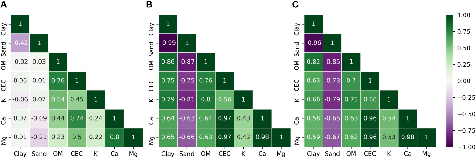
Figure 4 Pearson correlation matrix of laboratory analysis from soil samples that composed the three strategies of datasets used in this study. (A) Local dataset; (B) geological dataset; (C) global dataset.
The results for k-fold cross-validation of local, geological, and global prediction models are presented in Table 1. The local model usually performed its best prediction using fewer principal components than geological and global calibrations. Lower values for prediction errors (RMSE and MAE) were observed for the local model for all soil attributes predicted, except OM. On the other hand, R2 and RPIQ values for geological and global models overcame the local strategy, which presented R2 >0.60 for only OM and CEC and its best RPIQ of 1.35 for Ca prediction, while both geological and global models surpassed RPIQ = 2.00 for all attributes predicted.
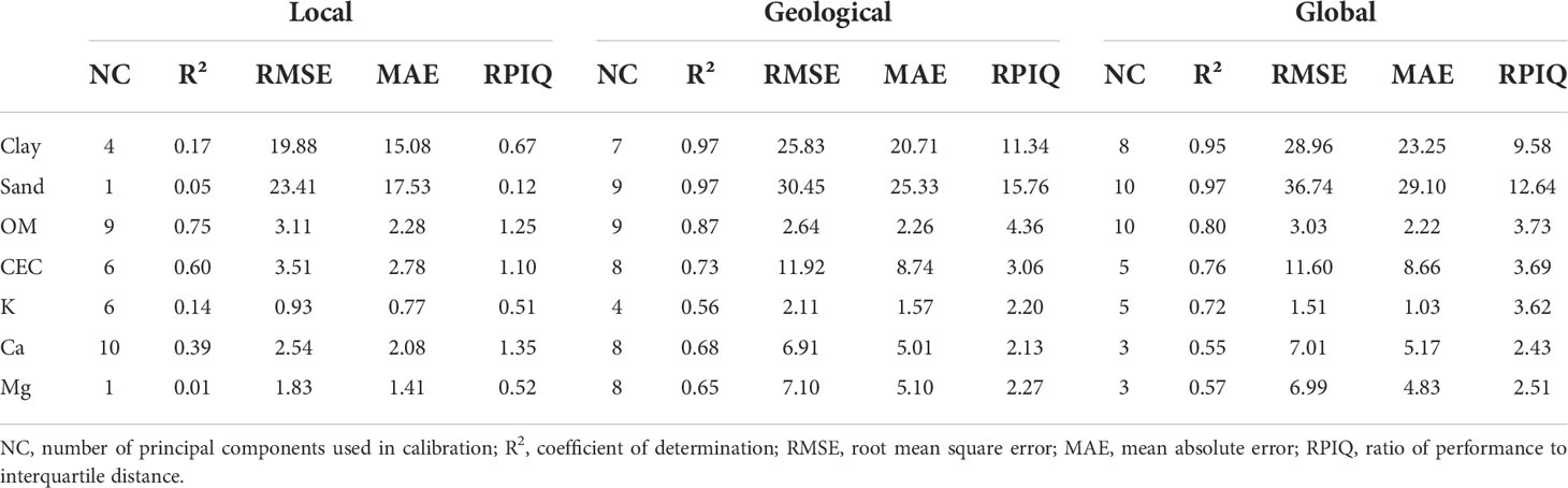
Table 1 Results of online prediction of soil clay, sand, organic matter (OM), cation exchange capacity (CEC), and calcium (Ca) using principal components regression (PCR) models developed for the different calibration strategies of only in-field samples (local), adding samples from the same geological region (geological), and from different geological regions (global).
Note that RPIQ values variation follows R2 values, departing from the prediction error presented by the model, since the smallest errors of the local model were not accompanied by better RPIQ values. This may imply that another parameter is needed to fully comprehend if the prediction model is sufficiently assertive to be used as a field technique for soil data acquisition. Agriculture is an activity that depends on the soil and its characteristics in deciding on productive steps. Not only the statistical distribution but also knowing the soil attributes content in the determined location is crucial for decision making (15). The spatial dependence of an attribute is known to be described by geostatistics, fitting variograms with the samples of the area (29). In this sense, it is suggested that the comprehension of the predicted values variation can contribute to a precise decision-making process of DRS NIR as a technique applied in the context of PA, both in quantitative terms, by the error of prediction, and in qualitative terms, by evaluating the spatial distribution of predicted values.
However, before evaluating the models in terms of variation in values observed, defining what is implied in the construction of soil attributes ML models is needed. A set of 72 soil samples from the nearby area located in Piracicaba (SP, Brazil) added to build geological and global datasets was divided and submitted for analysis to four different commercial laboratories, aiming to verify the difference in values that a standard laboratory analysis of a soil sample can present. A mean variation of 21.4 g kg−1 for clay content and 24.4 g kg−1 for sand content was observed between the analysis of the four laboratories. For chemical attributes, the results were even more discrepant. The analysis of OM and CEC exhibited a maximum Pearson correlation coefficient of 0.51 between laboratories. It is noteworthy that the mean error of prediction of the models calibrated in this study presented lower values than the variation observed among the different laboratories. The complete analysis of the 72 soil samples from the four laboratories is available in (20).
The certification of soil analytical laboratories in international level is a competence of the International Organization for Standardization (ISO) (30, 31). The standards of procedures and certification include acceptable errors and calibration limits for soil testing. This means that every analysis, even from certified laboratories, is susceptible to errors in some scale, and stakeholders of agriculture production always dealt with these possible variations.
Finding the correct values instead of generalizing attributes and variability is an obvious goal of PA (14), but the calibration of ML models depends on the reference values inserted in the calibration. DRS is directly related to the intrinsic content of an attribute of response in the determined electromagnetic spectrum region (3, 32). Thus, if there is no consensus in the value inserted for calibration, a misbalance of predicted versus observed values occurs, and the models automatically incorporate errors of prediction in some magnitude. This could imply that while we use this basis for ML models using DRS in soil science (33), we will hardly reach an accuracy level that allows to find the exact same values due to the model input, one of the three main sources that can lead to output uncertainty (34). Instead, we should aim to minimize the errors of prediction as much as possible and look forward to the repeatability of distribution and the agronomic plausibility of predicted attributes distribution, assuming that variations of some kind, already present in current analytical methods used, will not overcome the benefits that the technique can offer. Therefore, we suggest that evaluating the predicted attributes in quantiles associated with the prediction errors (35–37) is an effective approach rather than equalizing categories (17, 38, 39).
PCR models presented a described characteristic of this statistical method of smoothing predicted values when compared to those inserted in calibration (7) (Table 2). Besides the loss of extreme values of all datasets, the major portion of the population followed the distribution (6) (Figure 5). For clay and Mg prediction, the local model caused the major concentration of values when compared to geological and global predictions. The global model followed the exact range of values observed in the laboratory for its clay prediction.
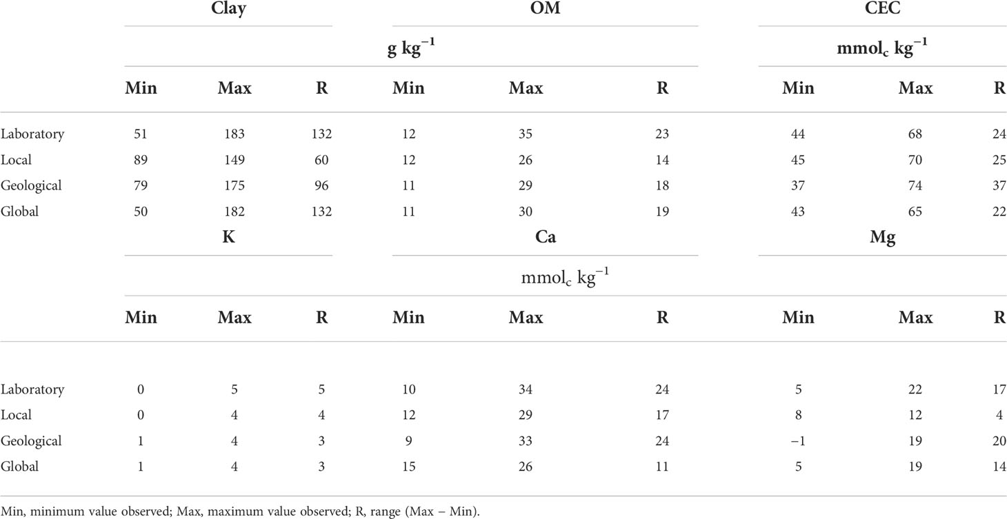
Table 2 Range of values observed for clay, organic matter (OM), cation exchange capacity (CEC), potassium (K), calcium (Ca), and magnesium (Mg) in laboratory analysis (Lab), and predicted values using online spectrum of experimental field from three different calibration strategies of only in-field samples (local), adding samples from the same geological region (Geo), and from different geological regions (global).
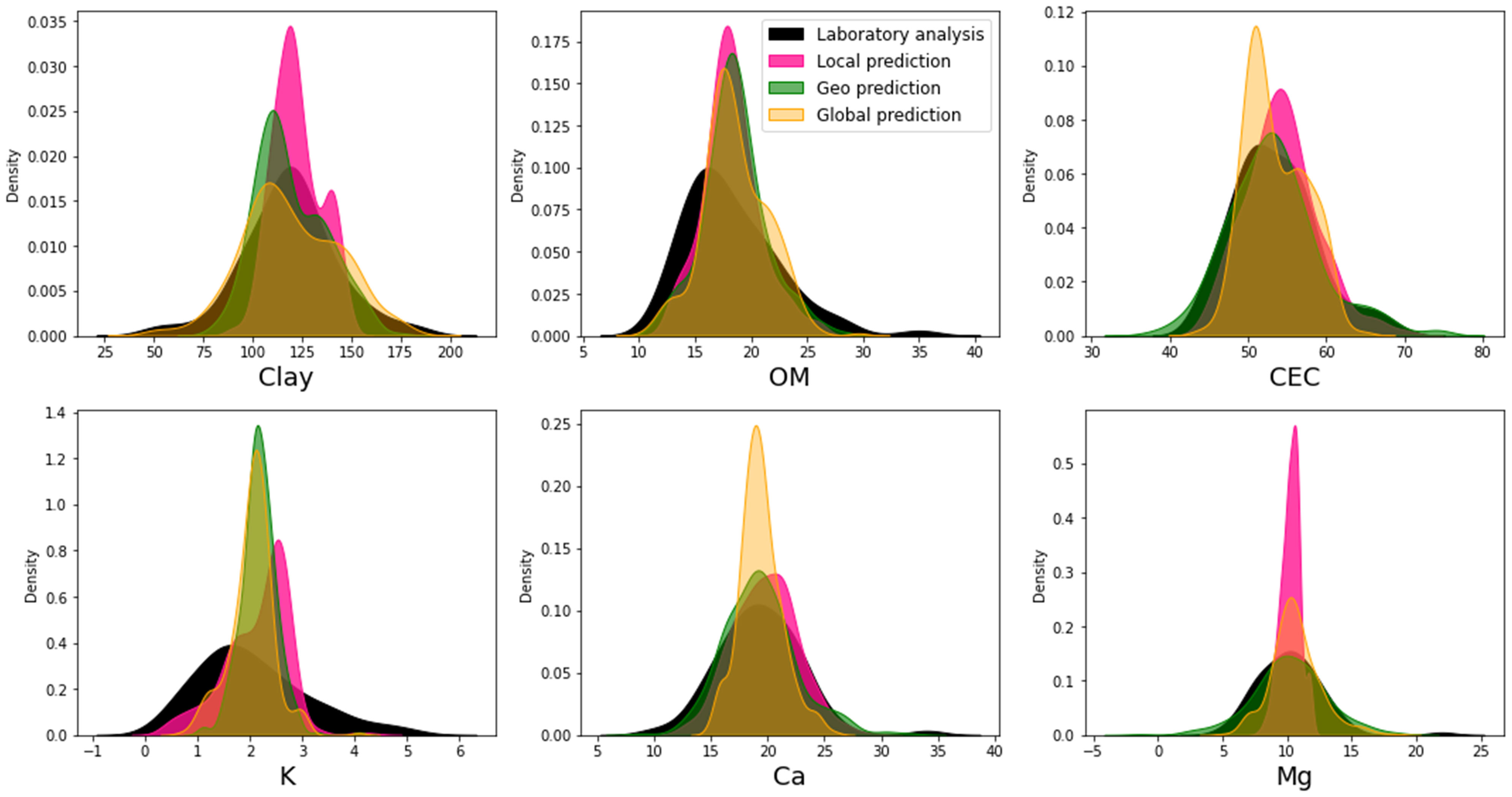
Figure 5 Kernel density estimate plots of clay, organic matter (OM), cation exchange capacity (CEC), potassium (K), calcium (Ca), and magnesium (Mg) for the attributes observed in the laboratory analysis of experimental area and predicted using online spectra on three strategies of calibration: only in-field samples (local), adding samples from the same geological region (geological), and from different geological regions (global).
The global model presented the major concentration of values for Ca prediction. For OM and K, the three strategies presented similar population distribution, even though all three flattened the distribution curve observed in the values of laboratory analysis. CEC prediction is highlighted as the most similar distribution for all populations. Nevertheless, the range of predicted values places the local calibration as the closest to laboratory population.
The parameters of fitted variograms for clay, sand, OM, CEC, K, Ca, and Mg, using the three strategies of calibration, hardly presented similar values (Table 3). However, the nugget to total sill ratio (40) presented moderate spatial dependence for almost all predicted attributes. Only Ca prediction from the local dataset and sand prediction from the global dataset exhibited pure nugget effect, indicating the inexistence of spatial dependence on the distribution of these attributes contents on the experimental field. Regardless, for Ca, geological and global calibrations were able to find spatial dependence. The same was observed for sand, in which local and geological calibrations pointed spatial dependence. This indicates that the spatial distribution of predicted values can be affected depending on the calibration model, despite the prediction error presented, corroborating with the results found in (39).
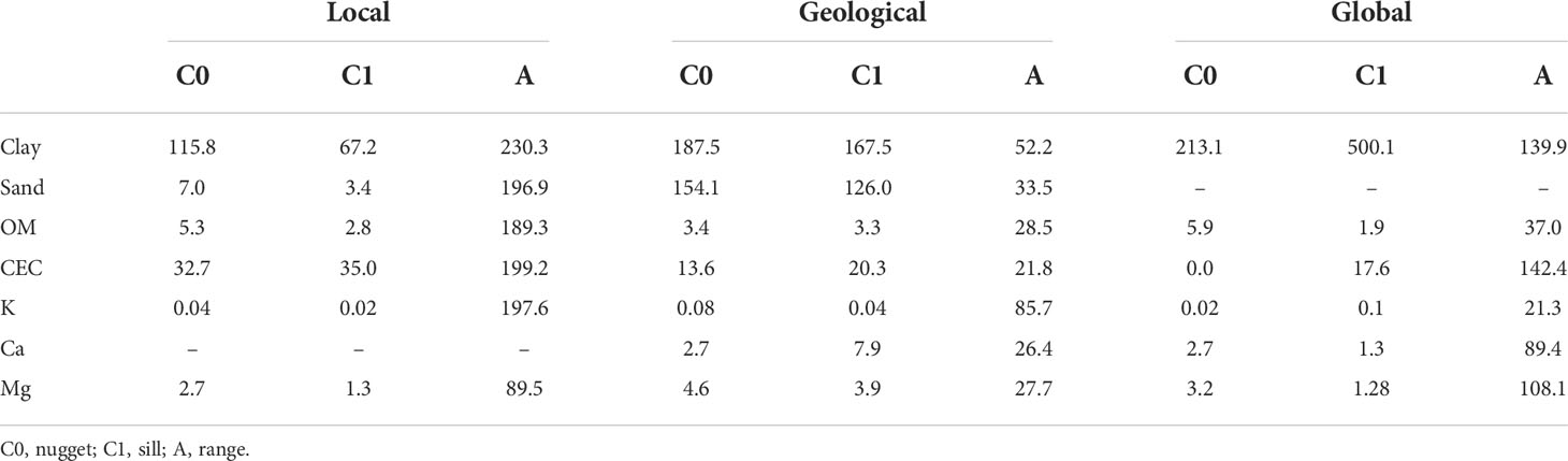
Table 3 Parameters of fitted variograms for clay, sand, organic matter (OM), cation exchange capacity (CEC), potassium (K), calcium (Ca), and magnesium (Mg) predicted values using online spectra of experimental field from three different calibration strategies of only in-field samples (local), adding samples from the same geological region (geological), and from different geological regions (global).
Clay prediction was not considerably affected by the addition of samples from outside areas, which could have happened due to the relation of clay and the fundamentals of NIR with soil mineralogy (32). Due to the direct response of this attribute in Vis-NIR, other authors even reported satisfactory prediction in independent tests, extrapolating predictive models in scanned but previous unsampled agricultural areas (41). The range presented by the three variograms fitted for clay prediction was discrepant: 230.3 m for local dataset, 52.2 m for geological dataset, and 139.9 m for the global dataset. Despite that, the ordinary kriging reached similar patterns and also similar values for the attribute (Figure 6), highlighting the variation amplitude observed in quantiles division, which is small. Class discrepancy of values was also lower than the MAE of prediction models (15.08 g kg−1 for local, 20.71 g kg−1 for geological, and 23.25 g kg−1 for global). The evaluation of R2 and RPIQ would lead to the discarding of clay local model. However, the spatial distribution of predicted values alongside the error of prediction proved the ability of the local calibration to predict this attribute of primary response in NIR.
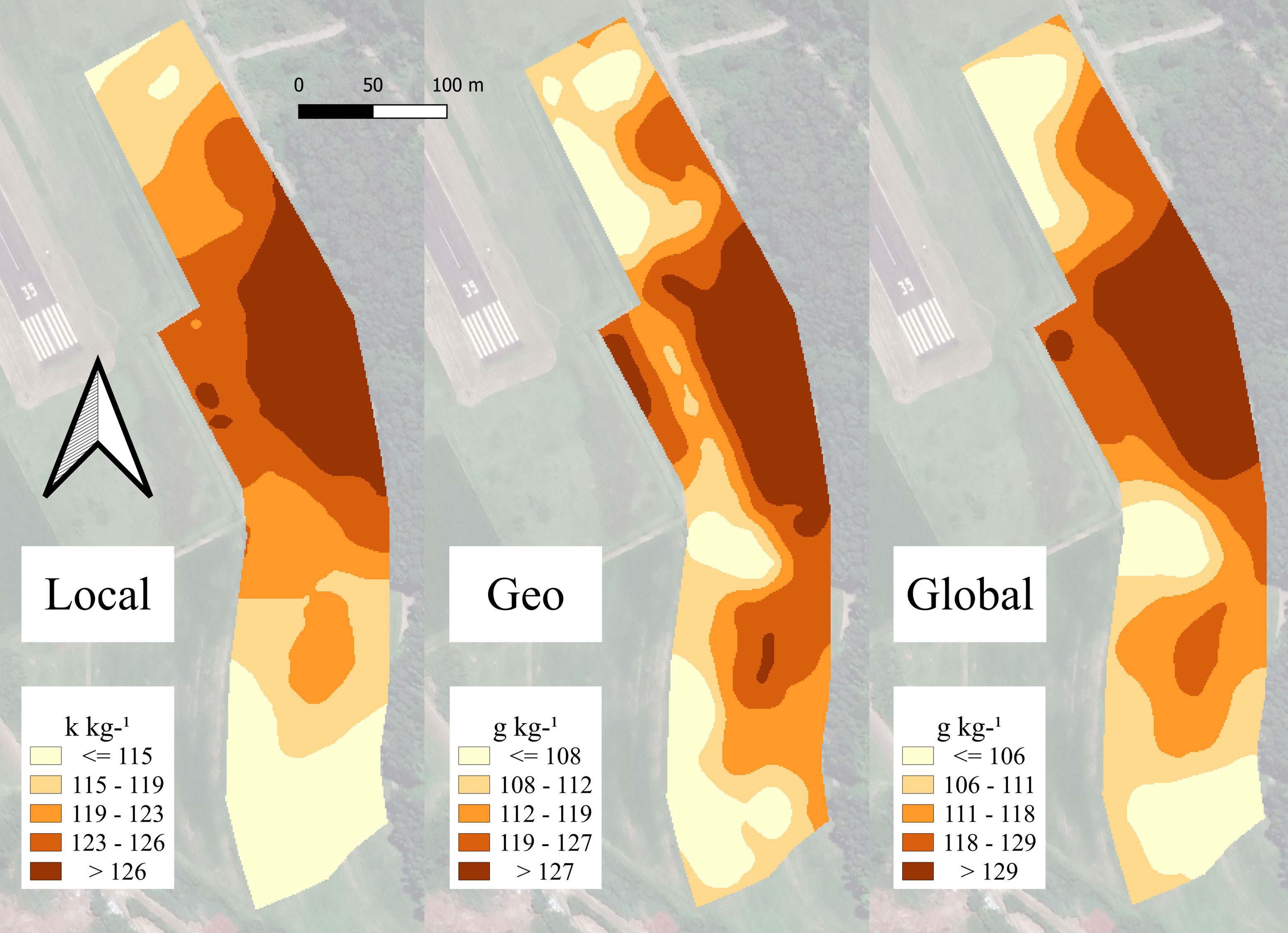
Figure 6 Maps of the five quantiles obtained by ordinary kriging for clay prediction using three different strategies of calibration only in-field samples (local), adding samples from the same geological region (geological), and adding samples from different geological regions (global).
The prediction of OM is widely explored using DRS NIR due to the fact that OM is a primary response attribute in this region of electromagnetic spectrum, with its typical wavelength absorption being reported to comprise (nm) 1,660, 1,728, 1,754, 20,56, 2,264, 2,306, and 2,347 (42). Its prediction can also arise in moist soil (not in field capacity) (43), a condition often observed in field soils. This is the most likely explanation for the satisfactory prediction of OM using the local, geological, and global dataset calibrations (Figure 7). Although with different calibrations, the models reached similar patterns of distribution, which was also observed by Pouladi et al. (39). As was observed for clay, the variation amplitude in quantiles distribution is small for OM prediction. The most divergent area was observed in the northwest portion of the field, where the local calibration pointed a zone of high OM content and geological and global calibrations pointed the opposite. In addition, the addition of outside samples in the calibration set clearly affected the spatial dependence of prediction of OM, since the range of the variograms expressively decreased. For local calibration, a spatial dependence until 189.3 m of distance was observed from one sampling point to another. For geological and global calibration, however, the spatial dependence was found until 28.5 and 37.0 m.
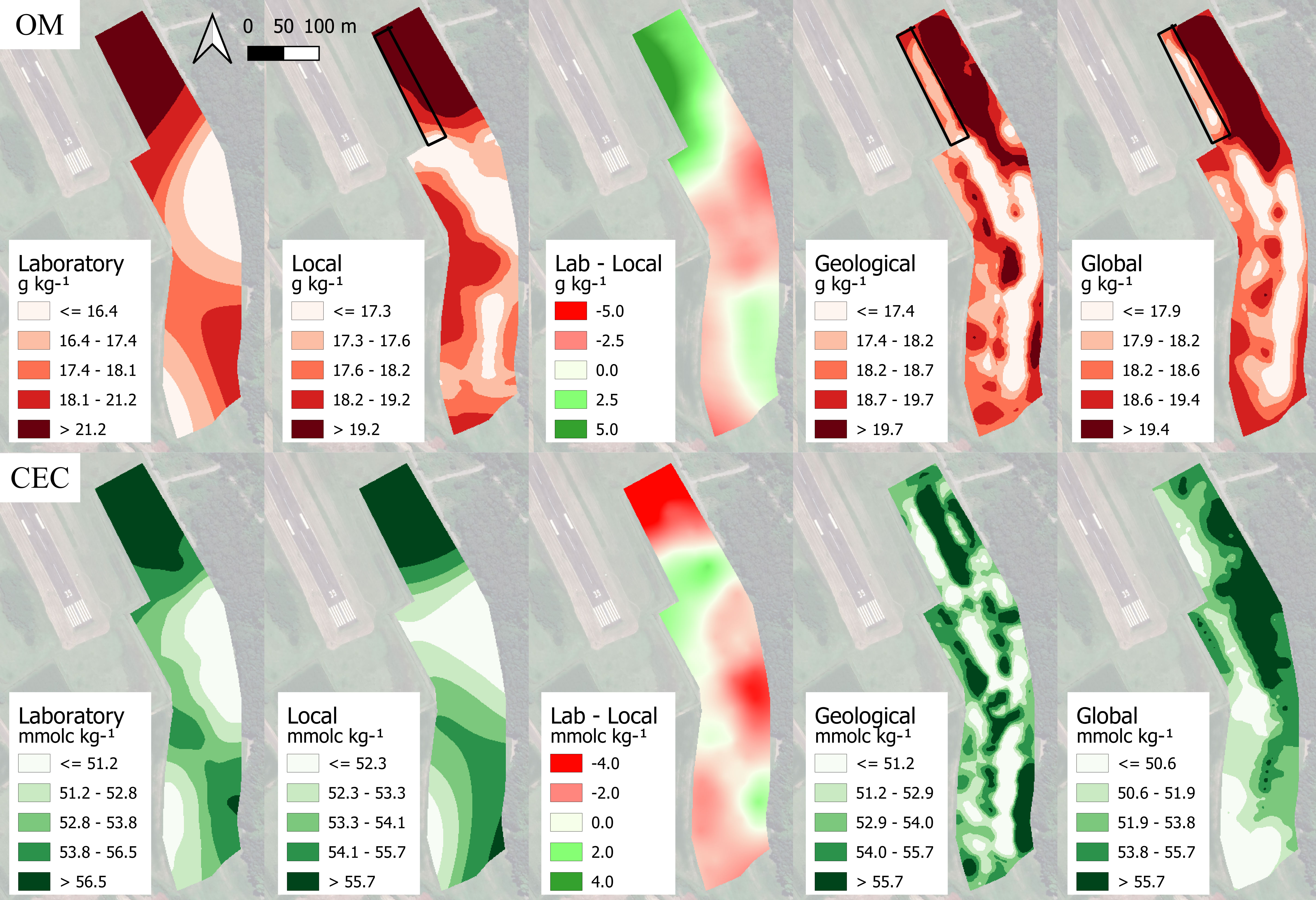
Figure 7 Maps of the five quantiles obtained by ordinary kriging of organic matter (OM), in red, and cation exchange capacity (CEC), in green. Maps are presented in the order of: laboratory analysis; prediction model calibrated with only in-field samples (local); difference of laboratory and local values (Lab − Local); prediction model calibrated adding samples from the same geological region (geological) and adding samples from different geological regions (global).
Although there were similarities among the maps of local, geological, and global calibrations, when comparing the map generated from the high density of 72 soil samples analyzed in the laboratory, it is noted that the local model presented the best fitted prediction for OM in the experimental field, similar to that reported by Stevens et al. (44). An explanation for local better prediction can be that changes in iron oxide content can cancel variations in OM absorption features (45). The major portion of the area presented a difference of <2.5 g kg−1. The greatest difference was observed in the same region that the local model disagreed with geological and global calibrations. Exactly in this region, laboratory analysis presented a single sample with 35 g kg−1 of OM content. The second highest OM content observed in the laboratory was 28 g kg−1. The upper limit loss in the range presented for local calibration was clearly affected for this sample only (Table 2). The errors of prediction of this model (MAE = 2.28 g kg−1 and RMSE = 3.11 g kg−1) were also increased due to what was quoted. Thus, it is assumed that a resampling of that area is needed to verify if the sample of 35 g kg−1 was accurate or it was an outlier due to the error in the sampling procedure/laboratory analysis (46). Nevertheless, if laboratory analysis predicted greatest values than the local model, which classified the area as a high content one, geological and global calibrations are wrong in the assumption of a low OM content area.
CEC prediction was discrepant between the three models (Figure 7). The geological model reached an irregular distribution of patterns in the field. While local calibration presented a variogram range of 199.2 m and global calibration of 142.4 m, the geological model reduced the range to 21.8 m. The difference between local and global prediction stands for the inversion of patterns observed, changing high CEC values zones into low ones. Although the range of 24 mmolc kg−1 in CEC values was observed in the laboratory, followed by three datasets predictions (Table 2), the quantiles limits presented a small variation of 1.5–2.0 mmolc kg−1.
Attributes that do not have direct spectral response in the region studied can be predicted if the attribute presents covariation with another of primary response (16). Thus, various authors have dedicated their attention to construct indirect Vis-NIR calibrations to predict these soil attributes (23, 47, 48). The use of calibrations that compile soil samples from different areas to predict these attributes is a common practice, usually gathering data from the same morphopedological region (16). Nevertheless, the strategy of putting together the areas from different regions is also observed and stated as an effective approach depending on the results demonstrated (49). In this study, although smaller prediction errors were obtained from local model prediction of CEC, geological and global models presented better R2 and RPIQ and metrics similar to others (18, 50, 51). However, it is noted that the values obtained from different strategies led to different patterns of attributes spatialization in the field, affecting the spatial dependence as for the geological model or the inversion of patterns as for the global model.
The comparison between the kriging maps obtained for CEC analysis in the laboratory and that obtained using local model calibration leads to the conclusion that the local model was the only strategy among the three that successfully predicted the attribute. At the north of the area, the region of greatest discrepancy was observed, where even though the model accurately defined the region of higher CEC at the field, it downsized the value observed by the laboratory analysis, smoothing the characteristics reported for PCR prediction models (7). It is highlighted that, although there was a small range of CEC values from both laboratory analysis (24 mmolc kg−1) and local prediction (25 mmolc kg−1) and a small variation amplitude in quantiles division, the local calibration was able to accurately identify the spatial patterns in the field.
The failure of the prediction of CEC for geological and global models, despite the considered good metrics presented by these two strategies, can be explained by the correlation observed between soil attributes (52) (Figure 4). For only the experimental area, CEC had a strong correlation with OM of 0.76, which is a primary response attribute in NIR. Note that in the experimental area, CEC is almost independent from clay, with a correlation coefficient of −0.06. By the addition of samples from the area of the same geological region than the experimental field, the correlation of CEC with OM is maintained at 0.76. Yet, the model identifies a strong correlation with other primary NIR response attributes, where CEC and clay had a correlation coefficient of 0.75. The similar effect happened for the global dataset. Although the KDE plots pointed the same statistical distribution of predicted values for all datasets (laboratory analysis, and local, geological, and global predictions) (Figure 5) and satisfactory metrics were presented (R2, RMSE, MAE, and RPIQ) (Table 1), the prediction of CEC with neither geological nor global models was accurate, which places spatial distribution and agronomic plausibility of this distribution as a fundamental factor for classifying the model as robust or not. Even though other authors found a positive influence of creating calibrations from multiple fields (23, 53), this was not the case for the one tested in this study when the field spatialization parameter was taken into account. This could also be possible due to the use of other techniques more related to fundamental vibrations of soil attributes in the spectra, like mid-infrared (MIR) (54) or X-ray fluorescence (55), or other factors that were not investigated in this study.
The prediction of plant nutrients was not consistent for any of the datasets used for model calibration, and Ca maps represented the same values observed for K and Mg (Figure 8). Local and geological datasets resulted in a prediction without coherent spatial patterns, and for the global dataset, although the north portion of the area presented the same pattern and similar values to those observed in the laboratory, it may be assigned by chance, once the other patterns were not steady.
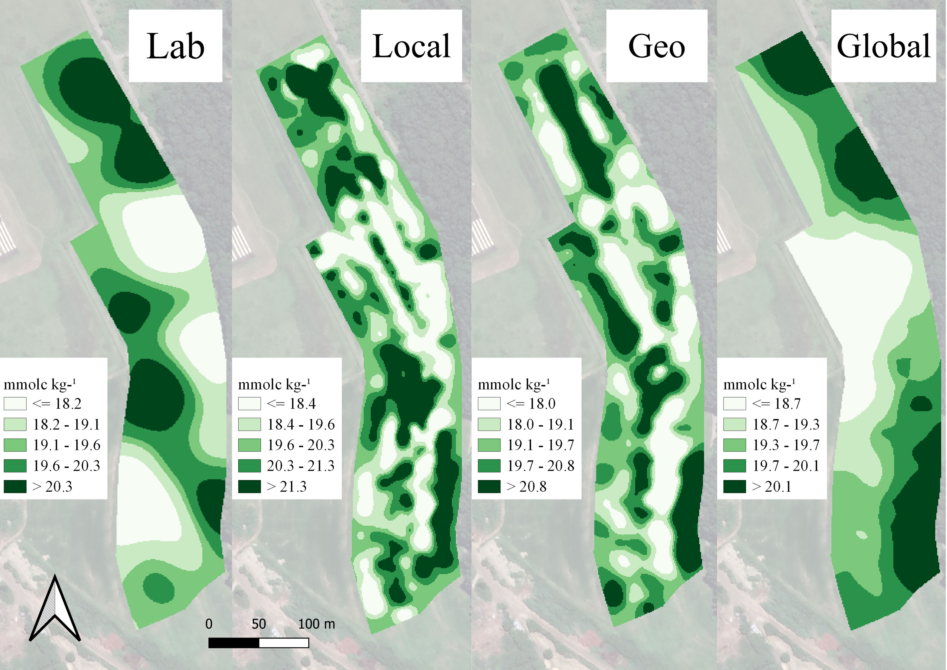
Figure 8 Maps of the five quantiles obtained by ordinary kriging of calcium (Ca) values of laboratory samples analysis (Lab) and the prediction models using three different strategies of calibration: only in-field samples (local), adding samples from the same geological region (geological), and adding samples from different geological regions (global).
The unsuccessful prediction of Ca can be related to the correlations presented for this attribute (Figure 4), as it was for the successful prediction of CEC (16, 52). In the experimental field, Ca had an average correlation with OM of 0.44. This fact could explain the slightly better R2 and RPIQ values presented in the validation of local Ca model, although this was not true for K (Table 1), even with a 0.55 positive correlation with OM presented in the local dataset. Nevertheless, this correlation magnitude proved to be insufficient to allow an accurate prediction using DRS NIR. For geological and global models, once outside samples were entered in the dataset, nutrient correlations were modified, presenting, in both cases, significant positive correlation with clay and OM and negative correlation with sand. Therefore, the ML models used in this study, which are helpful tools to deal with spectral data and correlations between soil attributes (33), were not able to perform a consistent prediction.
This study suggests that the correlation coefficient itself, even when corroborated with satisfactory statistical metrics on prediction models validation, cannot identify if a secondary response attribute can be predicted with DRS ML models (56). The correlation observed in the target area alone must be taken into account, and it is of high importance that this correlation is not twisted after the union of outside samples in the model calibration, which can cause the distortion of the attributes spatial distribution in the field.
Spatial distribution in terms of zones and agronomic plausibility of predicted values obtained from DRS NIR prediction models proved to be a key factor of robustness evaluation. Using R2 and RPIQ without field spatialization is suggested to be a vulnerable strategy due to misleading decisions that these metrics would lead into in the present study. This study suggests to further investigate the spatialization of soil attributes predicted using NIR spectra in areas with greater variability. It is necessary to further check the weaknesses that ML models of NIR spectra calibrated with samples from more than one area presented in the spatialization of the predicted attributes. If the observed results in the present study are repeated for other agricultural fields, it may indicate that local models are the best recommendation for DRS used for field-scale PSS.
The raw data supporting the conclusions of this article will be made available by the authors, without undue reservation.
RF contributed to the conceptualization, methodology, field testing, data analysis and modeling, and writing—original draft and editing. JM contributed to the conceptualization, methodology, writing—reviewing, supervision of the project, and partnership and funding acquisitions. All authors contributed to the article and approved the submitted version.
Soil sample analyses were funded by the Brazilian Institute of Analysis (IBRA). The sensor was offered from a partnership with Spectral Solutions (São Paulo, Brazil). RCF was funded by the National Council for Scientific and Technological Development (CNPq) – project 830707/1999-9.
The authors declare that the research was conducted in the absence of any commercial or financial relationships that could be construed as a potential conflict of interest.
All claims expressed in this article are solely those of the authors and do not necessarily represent those of their affiliated organizations, or those of the publisher, the editors and the reviewers. Any product that may be evaluated in this article, or claim that may be made by its manufacturer, is not guaranteed or endorsed by the publisher.
The Supplementary Material for this article can be found online at: https://www.frontiersin.org/articles/10.3389/fsoil.2022.984963/full#supplementary-material
1. Viscarra Rossel RA, Adamchuk VI, Sudduth KA, McKenzie NJ, Lobsey C. Proximal soil sensing. An effective approach for soil measurements in space and time. Adv Agronomy. (2011) 113:243–91. doi: 10.1016/B978-0-12-386473-4.00005-1
2. Wang D, Chakraborty S, Weindorf DC, Li B, Sharma A, Paul S, et al. Synthesized use of VisNIR DRS and PXRF for soil characterization: Total carbon and total nitrogen. Geoderma (2015) 243:157–67. doi: 10.1016/j.geoderma.2014.12.011
3. Pasquini C. Near infrared spectroscopy: A mature analytical technique with new perspectives – a review. Analytica Chimica Acta (2018) 1026:8–36. doi: 10.1016/j.aca.2018.04.004
4. Molin JP, Tavares TR. Sensor systems for mapping soil fertility attributes: Challenges, advances, and perspectives in brazilian tropical soils. Engenharia Agricola (2019) 39(specialissue):126–47. doi: 10.1590/1809-4430-eng.agric.v39nep126-147/2019
5. Williams P, Norris K. Near-infrared technology in the agricultural and food industries. St. Paul, Minnesota: American Association of Cereal Chemists, Inc (1987) p. 330. Available at: https://www.cabdirect.org/cabdirect/abstract/19892442443.
6. Velliangiri S, Alagumuthukrishnan S, Thankumar Joseph SI. A review of dimensionality reduction techniques for efficient computation. Procedia computer science (2019) 165:104–11. doi: 10.1016/j.procs.2020.01.079
7. Bellon-Maurel V, Fernandez-Ahumada E, Palagos B, Roger JM, McBratney A. Critical review of chemometric indicators commonly used for assessing the quality of the prediction of soil attributes by NIR spectroscopy. TrAC - Trends Analytical Chem (2010) 29:1073–81. doi: 10.1016/j.trac.2010.05.006
8. Chang CW, Laird DA, Mausbach MJ, Hurburgh CR. Near-infrared reflectance spectroscopy-principal components regression analyses of soil properties. Soil Sci Soc America J (2001) 65(2):480–90. doi: 10.2136/sssaj2001.652480x
9. Morellos A, Pantazi XE, Moshou D, Alexandridis T, Whetton R, Tziotzios G, et al. Machine learning based prediction of soil total nitrogen, organic carbon and moisture content by using VIS-NIR spectroscopy. Biosyst Engineering. (2016) 152:104–16. doi: 10.1016/j.biosystemseng.2016.04.018
10. Christy CD. Real-time measurement of soil attributes using on-the-go near infrared reflectance spectroscopy. Comput Electron Agriculture. (2008) 61(1):10–9. doi: 10.1016/j.compag.2007.02.010
11. Barthès BG, Brunet D, Hien E, Enjalric F, Conche S, Freschet GT, et al. Determining the distributions of soil carbon and nitrogen in particle size fractions using near-infrared reflectance spectrum of bulk soil samples. Soil Biol Biochem (2008) 40(6):1533–37. doi: 10.1016/j.soilbio.2007.12.023
12. Wang Y, Huang T, Liu J, Lin Z, Li S, Wang R, et al. Soil pH value, organic matter and macronutrients contents prediction using optical diffuse reflectance spectroscopy. Comput Electron Agriculture. (2015) 111:69–77. doi: 10.1016/j.compag.2014.11.019
13. Vishwakarma G, Sonpal A, Hachmann J. Metrics for benchmarking and uncertainty quantification: Quality, applicability, and best practices for machine learning in chemistry. Trends Chem (2021) 3:146–56. doi: 10.1016/j.trechm.2020.12.004
14. International Society of Precision Agriculture. Precision agriculture definition. (2022). Available at: https://www.ispag.org/about/definition. [Acessed Jul 01, 2022]
15. Abdel Rahman MAE, Zakarya YM, Metwaly MM, Koubouris G. Deciphering soil spatial variability through geostatistics and interpolation techniques. Sustainability (Switzerland). (2021) 13(1):194. doi: 10.3390/su13010194
16. Stenberg B, Viscarra Rossel RA, Mouazen AM, Wetterlind J. Visible and near infrared spectroscopy in soil science. Adv Agron (2010) 107:163–215. doi: 10.1016/S0065-2113(10)07005-7
17. Franceschini MHD, Demattê JAM, Kooistra L, Bartholomeus H, Rizzo R, Fongaro CT, et al. Effects of external factors on soil reflectance measured on-the-go and assessment of potential spectral correction through orthogonalisation and standardisation procedures. Soil Tillage Res (2018) 177:19–36. doi: 10.1016/j.still.2017.10.004
18. Ulusoy Y, Tekin Y, Tümsavaş Z, Mouazen AM. Prediction of soil cation exchange capacity using visible and near infrared spectroscopy. Biosyst Engineering. (2016) 152:79–93. doi: 10.1016/j.biosystemseng.2016.03.005
19. Guerrero A, de Neve S, Mouazen AM. Data fusion approach for map-based variable-rate nitrogen fertilization in barley and wheat. Soil Tillage Res (2021) 205:104789–803. doi: 10.1016/j.still.2020.104789
20. Eitelwein MT. Proximal soil sensing: quantification of physical and chemical soil attributes. Piracicaba: Luiz de Queiroz College of Agriculture - University of São Paulo (2017).
21. Kluyver T, Ragan-Kelley B, Pérez F, Granger B, Bussonnier M, Frederic J, et al. Jupyter notebooks–a publishing format for reproducible computational workflows. In: Positioning and power in academic publishing: Players, agents and agendas - proceedings of the 20th international conference on electronic publishing,. (Göttingen, Germany: ELPUB) (2016) 2016.
23. Munnaf MA, Nawar S, Mouazen AM. Estimation of secondary soil properties by fusion of laboratory and on-line measured vis-NIR spectra. Remote Sensing. (2019) 11(23):2819–41. doi: 10.3390/rs11232819
24. Zhang J, Guerrero A, Mouazen AM. Map-based variable-rate manure application in wheat using a data fusion approach. Soil Tillage Res (2021) 207:104846–58. doi: 10.1016/j.still.2020.104846
25. Jung Y. Multiple predicting K-fold cross-validation for model selection. J Nonparametric Statistics. (2018) 30(1):197–215. doi: 10.1080/10485252.2017.1404598
26. Minasny B, McBratney AB, Whelan BM. VESPER version 1.62. Sidney: Australian Centre for Precision Agriculture (2006).
27. QGIS Development Team. (2022). QGIS Geographic Information System. Open Source Geospatial Foundation.
28. Syers JK, Campbell AS, Walker TW. Contribution of organic carbon and clay to cation exchange capacity in a chronosequence of sandy soils. Plant Soil. (1970) 33(1):104–12. doi: 10.1007/BF01378202
29. de Iaco S, Hristopulos DT, Lin G. Special issue: Geostatistics and machine learning. Math Geosciences. (2022) 54(3):459–65. doi: 10.1007/s11004-022-09998-6
30. International Organization for Standardization. General requirements for the competence of testing and calibration laboratories (2022). Available at: https://www.iso.org/standards.html.
31. International Organization for Standardization. Laboratory testing of soi (2022). Available at: https://www.iso.org/standards.html.
32. Fang Q, Hong H, Zhao L, Kukolich S, Yin K, Wang C. Visible and near-infrared reflectance spectroscopy for investigating soil mineralogy: A review. J Spectrosc (2018) 2018:1–14. doi: 10.1155/2018/3168974
33. Barra I, Haefele SM, Sakrabani R, Kebede F. Soil spectroscopy with the use of chemometrics, machine learning and pre-processing techniques in soil diagnosis: Recent advances–a review. TrAC - Trends Analytical Chem (2021) 135:116116–29. doi: 10.1016/j.trac.2020.116166
34. Huang J, Zare E, Malik RS, Triantafilis J. An error budget for soil salinity mapping using different ancillary data. Soil Res (2015) 53(5):561–75. doi: 10.1071/SR15043
35. Malone BP, McBratney AB, Minasny B. Empirical estimates of uncertainty for mapping continuous depth functions of soil attributes. Geoderma (2011) 160(3–4):614–26. doi: 10.1016/j.geoderma.2010.11.013
36. Vaysse K, Lagacherie P. Using quantile regression forest to estimate uncertainty of digital soil mapping products. Geoderma. (2017) 291:55–64. doi: 10.1016/j.geoderma.2016.12.017
37. Ma Y, Minasny B, Wu C. Mapping key soil properties to support agricultural production in Eastern China. Geoderma Regional. (2017) 10:144–53. doi: 10.1016/j.geodrs.2017.06.002
38. Somarathna PDSN, Malone BP, Minasny B. Mapping soil organic carbon content over new south Wales, Australia using local regression kriging. Geoderma Regional. (2016) 7(1):38–48. doi: 10.1016/j.geodrs.2015.12.002
39. Pouladi N, Møller AB, Tabatabai S, Greve MH. Mapping soil organic matter contents at field level with cubist, random forest and kriging. Geoderma. (2019) 342:85–92. doi: 10.1016/j.geoderma.2019.02.019
40. Cambardella CA, Moorman TB, Novak JM, Parkin TB, Karlen DL, Turco RF, et al. Field-scale variability of soil properties in central Iowa soils. Soil Sci Soc America J (1994) 58(5):1501–11. doi: 10.2136/sssaj1994.03615995005800050033x
41. Eitelwein MT, Tavares TR, Molin JP, Trevisan RG, de Sousa RV, Demattê JAM. Predictive performance of mobile vis–NIR spectroscopy for mapping key fertility attributes in tropical soils through local models using PLS and ANN. Automation. (2022) 3(1):116–31. doi: 10.3390/automation3010006
42. Nocita M, Stevens A, van Wesemael B, Aitkenhead M, Bachmann M, Barthès B, et al. Soil spectroscopy: An alternative to wet chemistry for soil monitoring. Adv Agronomy. (2015) 132:139–59. doi: 10.1016/bs.agron.2015.02.002
43. Wang YP, Lee CK, Dai YH, Shen Y. Effect of wetting on the determination of soil organic matter content using visible and near-infrared spectrometer. Geoderma. (2020) 376:114528–39. doi: 10.1016/j.geoderma.2020.114528
44. Stevens A, Nocita M, Tóth G, Montanarella L, van Wesemael B. Prediction of soil organic carbon at the European scale by visible and near InfraRed reflectance spectroscopy. PloS One (2013) 8(6):66409–22. doi: 10.1371/journal.pone.0066409
45. Adar S, Shkolnisky Y, Ben-Dor E. Change detection of soils under small-scale laboratory conditions using imaging spectroscopy sensors. Geoderma. (2014) 216:19–29. doi: 10.1016/j.geoderma.2013.10.017
46. Hemingway RG. Soil-sampling errors and advisory analyses. J Agric Science. (1955) 46(1):1–8. doi: 10.1017/S0021859600039563
47. Bönecke E, Meyer S, Vogel S, Schröter I, Gebbers R, Kling C, et al. Guidelines for precise lime management based on high-resolution soil pH, texture and SOM maps generated from proximal soil sensing data. Precis Agriculture. (2021) 22(2):493–523. doi: 10.1007/s11119-020-09766-8
48. Pätzold S, Leenen M, Frizen P, Heggemann T, Wagner P, Rodionov A. Predicting plant available phosphorus using infrared spectroscopy with consideration for future mobile sensing applications in precision farming. Precis Agriculture. (2020) 21(4):737–61. doi: 10.1007/s11119-019-09693-3
49. Munnaf MA, Guerrero A, Nawar S, Haesaert G, van Meirvenne M, Mouazen AM. A combined data mining approach for on-line prediction of key soil quality indicators by vis-NIR spectroscopy. Soil Tillage Res (2021) 205:104808–20. doi: 10.1016/j.still.2020.104808
50. Rehman HU, Knadel M, Jonge LW, Moldrup P, Greve MH, Arthur E. Comparison of cation exchange capacity estimated from vis–NIR spectral reflectance data and a pedotransfer function. Vadose Zone J (2019) 18(1):1–8. doi: 10.2136/vzj2018.10.0192
51. Chen Y, Gao S, Jones EJ, Singh B. Prediction of soil clay content and cation exchange capacity using visible near-infrared spectroscopy, portable X-ray fluorescence, and X-ray diffraction techniques. Environ Sci Technology. (2021) 55(8):4629–37. doi: 10.1021/acs.est.0c04130
52. Kuang B, Mahmood HS, Quraishi MZ, Hoogmoed WB, Mouazen AM, van Henten EJ. Sensing soil properties in the laboratory, in situ, and on-line. a review. In: Advances in agronomy (London, UK: Academic Press) (2012).
53. Carmon N, Ben-Dor E. An advanced analytical approach for spectral - based modelling of soil properties. Int J Emerging Technol Advanced Engineering. (2017) 7(3):90–7.
54. Greenberg I, Seidel M, Vohland M, Koch HJ, Ludwig B. Performance of in situ vs laboratory mid-infrared soil spectroscopy using local and regional calibration strategies. Geoderma. (2022) 409:115614–29. doi: 10.1016/j.geoderma.2021.115614
55. Qu M, Liu H, Guang X, Chen J, Zhao Y, Huang B. Improving correction quality for in-situ portable X-ray fluorescence (PXRF) using robust geographically weighted regression with categorical land-use types at a regional scale. Geoderma. (2022) 409:115615–22. doi: 10.1016/j.geoderma.2021.115615
Keywords: soil variability, geostatistics, diffuse reflectance spectroscopy, machine learning, agriculture management
Citation: Canal Filho R and Molin JP (2022) Spatial distribution as a key factor for evaluation of soil attributes prediction at field level using online near-infrared spectroscopy. Front. Soil Sci. 2:984963. doi: 10.3389/fsoil.2022.984963
Received: 02 July 2022; Accepted: 13 September 2022;
Published: 03 October 2022.
Edited by:
Lingling Li, Gansu Agricultural University, ChinaReviewed by:
Mojtaba Zeraatpisheh, University of Vermont, United StatesCopyright © 2022 Canal Filho and Molin. This is an open-access article distributed under the terms of the Creative Commons Attribution License (CC BY). The use, distribution or reproduction in other forums is permitted, provided the original author(s) and the copyright owner(s) are credited and that the original publication in this journal is cited, in accordance with accepted academic practice. No use, distribution or reproduction is permitted which does not comply with these terms.
*Correspondence: Ricardo Canal Filho, cmljYXJkb2NhbmFsQHVzcC5icg==
Disclaimer: All claims expressed in this article are solely those of the authors and do not necessarily represent those of their affiliated organizations, or those of the publisher, the editors and the reviewers. Any product that may be evaluated in this article or claim that may be made by its manufacturer is not guaranteed or endorsed by the publisher.
Research integrity at Frontiers
Learn more about the work of our research integrity team to safeguard the quality of each article we publish.