Topsoil Texture Regionalization for Agricultural Soils in Germany—An Iterative Approach to Advance Model Interpretation

Gebauer, Anika; Sakhaee, Ali; Don, Axel; Poggio, Matteo; Ließ, Mareike

doi:10.3389/fsoil.2021.770326

ORIGINAL RESEARCH article

Front. Soil Sci., 04 January 2022

Sec. Pedometrics

Volume 1 - 2021 | https://doi.org/10.3389/fsoil.2021.770326

This article is part of the Research Topic Digital Soil Mapping - Advancing the Knowledge Frontiers View all 6 articles

Topsoil Texture Regionalization for Agricultural Soils in Germany—An Iterative Approach to Advance Model Interpretation

$\nAnika Gebauer$ Anika Gebauer¹^*

¹Department of Soil System Science, Helmholtz Centre for Environmental Research—UFZ, Halle (Saale), Germany
²Thünen Institute of Climate Smart Agriculture, Braunschweig, Germany

Site-specific spatially continuous soil texture data is required for many purposes such as the simulation of carbon dynamics, the estimation of drought impact on agriculture, or the modeling of water erosion rates. At large scales, there are often only conventional polygon-based soil texture maps, which are hardly reproducible, contain abrupt changes at polygon borders, and therefore are not suitable for most quantitative applications. Digital soil mapping methods can provide the required soil texture information in form of reproducible site-specific predictions with associated uncertainties. Machine learning models were trained in a nested cross-validation approach to predict the spatial distribution of the topsoil (0–30 cm) clay, silt, and sand contents in 100 m resolution. The differential evolution algorithm was applied to optimize the model parameters. High-quality nation-wide soil texture data of 2,991 soil profiles was obtained from the first German agricultural soil inventory. We tested an iterative approach by training models on predictor datasets of increasing size, which contained up to 50 variables. The best results were achieved when training the models on the complete predictor dataset. They explained about 59% of the variance in clay, 75% of the variance in silt, and 77% of the variance in sand content. The RMSE values ranged between approximately 8.2 wt.% (clay), 11.8 wt.% (silt), and 15.0 wt.% (sand). Due to their high performance, models were able to predict the spatial texture distribution. They captured the high importance of the soil forming factors parent material and relief. Our results demonstrate the high predictive power of machine learning in predicting soil texture at large scales. The iterative approach enhanced model interpretability. It revealed that the incorporated soil maps partly substituted the relief and parent material predictors. Overall, the spatially continuous soil texture predictions provide valuable input for many quantitative applications on agricultural topsoils in Germany.

Introduction

Soil texture is one of the most important physical soil properties. It influences, for example, the sequestration of carbon (1), it affects soil hydrological properties (2), and the susceptibility to soil erosion (3). Consequently, soil texture data is required to simulate the carbon dynamics of soils under different management practices (4–6), to estimate the drought impact on agriculture (7) or to model water erosion rates (8, 9). At large scales, site-specific information on the spatial continuous distribution of clay, silt, and sand contents is often missing. In many cases, existing polygon-based maps are not suitable for quantitative applications as they consist of complex compositions, are hardly reproducible, and represent only abrupt changes at polygon borders (10). Ließ et al. (11) discussed the limitation of conventional national German soil maps with regards to their usage in agricultural process models due to their composition of map units comprising various soil systematic units of differing properties and unspecified spatial allocation. Instead, predictive soil mapping methods can provide the required soil information in form of reproducible site-specific predictions with associated uncertainties (12).

Predictive soil mapping (also known as digital soil mapping) refers to the methodology for generating spatially continuous soil information by applying numerical or statistical models. Models are trained to extract the empirical relationship between soils and their properties gathered at specific locations (response variables) and the soil forming factors represented by spatially continuous data products (predictor variables). McBratney et al. (13), Scull et al. (14), and Zhang et al. (15) provide reviews. The approach is rooted in the ideas of Jenny (16) and Dokuchaev (17), who explained soil formation as a function of five soil forming factors: climate (C), organisms (O), relief (R), parent material (P), and time (A). McBratney et al. (13) extended the concept by adding other soil properties (S) and the spatial position (N), formalizing the scorpan approach. Nowadays, empirical models are trained on various scorpan factor proxies, for example, proximal and remote sensing data, interpolated meteorological observations, or, geology and soil maps (13, 15).

Overall, the usage of machine learning models in predictive soil mapping is increasing (18, 19). This can be attributed to their ability to deal with complex non-linear dependencies between predictor and response variables (20). Most soil texture predictions are done using tree-based machine learning algorithms. These include for example cubist decision tree models (21–23), random forest models (24–26), or boosted regression trees (27–29). Tree-based models have an important advantage over most other machine learning models: they allow the simple computation of the predictor importance and are therefore comparatively easy to interpret (18, 19, 30). Other machine learning algorithms used for the prediction of soil texture are support vector machines (31–33) and artificial neural networks (34–36). According to the no-free-lunch theorem, it can be assumed that all algorithms perform equally well on average (37). This is confirmed by comparisons of different machine learning models in soil texture predictions [e.g., (32, 35, 36)]; no model algorithm solved it all.

To fully exploit the potential of a machine learning algorithm, the usage of appropriate parameter tuning is essential (11). If the values of the tuning parameters can only be discrete integers, it is usually sufficient to try out a certain number of predefined values to adapt the machine learning algorithm to the specific modeling problem. This can be done by using a grid search, which is the standard method in predictive soil mapping (38–40). If the tuning parameters are continuous real numbers, exhaustive tuning requires numerical optimization algorithms [e.g., (11, 41)]. One technique that allows for the evaluation of the complete parameter space of real numbers is the differential evolution algorithm (42). It can outperform various other optimization algorithms (42–44) and has been applied successfully in soil science. For example, to tune the parameters of neural networks (45, 46), boosted regression trees (41), or geostatistical models (47).

Often the quality and quantity of the training data is the most influential factor in restricting model performance (18, 19, 48). First and foremost, the response variable dataset must be of high quality to avoid introducing uncertainty into the model (49). Second, its size has to be large enough to capture the complexity of the respective research area (19). Third, its size must fit model requirements as the sensitivity to the size of the training data set depends on the model algorithm (18). While a suitable sampling scheme and accurate quality control help to generate an appropriate response variable dataset, creating the predictor dataset is often more difficult. Most studies must rely on readily available spatial data (13, 15) whose quality can be difficult to verify (49). The scorpan factors that determine the spatial distribution of the response variable in a given research area must be represented by the predictor dataset to achieve reasonable results (12, 13). The number of predictors also depends on the number of sampled soil profiles. In order to represent the predictors well, a sufficiently large sample size is necessary.

The increase in computing capacity nowadays allows predictions at large scales (15, 48). Adhikari et al. (21), for example, trained a cubist tree model to predict the soil texture of Denmark. They used predictors derived from a digital elevation model (DEM) as well as soil, geology, and land use maps. Wadoux (50) applied a deep learning convolutional neural network to predict the soil texture of France. It was trained on coordinates, predictors derived from spectral images and a DEM as well as climate, land cover, and parent material maps. Liu et al. (51) trained a random forest model to predict the soil texture of China. They used predictors derived from a DEM and spectral images as well as climate and parent material maps. Ramcharan et al. (52) predicted the percentage of clay and sand of the conterminous Unites States using random forest and gradient boosting algorithms. The models were trained on predictors derived from a DEM and satellite images, climate data, soil property maps, land cover information as well as fire regime classes and aeroradiometric grids. The number of studies that focus on large-scale texture predictions of soils under agricultural land use is particularly scarce. One example is given by Piikki and Söderström (53), who predicted the topsoil texture of arable land in Sweden. High-resolution airborne gamma-ray spectrometry data, DEM derived predictors, and a geology map enabled them to obtain reasonable results.

The first predictive soil mapping study conducted at national scale, Germany, was presented by Ließ et al. (11). They trained support vector machine models to predict the spatial distribution of agricultural soil functional types at 100 m resolution. These were defined by various soil parameters along the depth profile and included soil texture data. However, until now, no machine learning model was specifically trained to predict the spatial texture distribution of agricultural topsoils throughout Germany. Models that were trained for larger scales and cover Germany provide predictions in comparatively low resolutions. Ballabio et al. (54), for example, used multivariate adaptive regression splines to predict the topsoil (0–20 cm) texture in 500 m resolution at continental scale (Europe). Their response variable dataset was derived from the topsoil database of the land use and cover area frame statistical (LUCAS) survey. Predictor variables incorporated remotely sensed vegetation indices, DEM derived variables, land cover information as well as temperature and precipitation data. Hengl et al. (55) used various machine learning models to predict the soil texture distribution in 250 m resolution at global scale. Predictions were done for seven depths: 0, 5, 15, 30, 60, 100, and 200 cm. Their response variable dataset was derived from various sources including the LUCAS topsoil database. Predictor variables incorporated, among others, remotely sensed spectral images, DEM derived variables, land cover information, precipitation data, lithologic units, landform classes as well as information on soil and sedimentary deposit thickness.

This is the first study that deals exclusively with the spatial prediction of the topsoil texture (0–30 cm) of agricultural soils in Germany. Machine learning models were trained to predict clay, silt, and sand contents in 100 m resolution. We tested an iterative approach to enhance model interpretability: models were trained on predictor datasets of increasing size.

Materials and Methods

Response Variable Datasets

Models were trained with regards to three response variables: clay, silt, and sand content of the top 30 cm which will be referred to as topsoil throughout this manuscript. We refrained from treating clay, silt, and sand as compositional variables, as their transformation can result in biased predictions (26). The required data was obtained from the harmonized database of the first German agricultural soil inventory (56). For a description of the inventory, including details on the soil analysis and their results please refer to the report of Jacobs et al. (57). Briefly, 3,104 soil profiles under agricultural land use (croplands, permanent grassland, and special crops) were selected based on a German-wide 8 km raster. Their topsoil was sampled from two depth intervals while taking horizon boundaries into account: 0–10 and 10–30 cm. Among other lab measurements, the database includes the mass of fine soil (<2,000 μm) as well as the contents of clay (<2 μm), three silt fractions (2–6.3, 6.3–20, 20–63 μm) and three sand fractions (63–200, 200–630, and 630–2,000 μm). Clay, silt, and sand contents were determined by applying the sieve and sedimentation method according to DIN ISO11277 (58). The fine soil mass was calculated from the dry bulk density according to HFA A2.8 (59).

We extracted the topsoil clay, total silt (2–63 μm), and total sand (63–2,000 μm) contents as well as the fine soil mass from the database. Excluding sites with missing data—mostly peat soils and soils with high organic matter contents—, we used topsoil data from 2,991 sites. Likely due to the agricultural land use, the texture in most profiles barely differed in the first 30 cm (57). Consequently, we combined the texture data from the topsoil into a weighted mean per soil profile. The fine soil mass was used as the weighting factor.

Research Area and Predictor Datasets

Our research focuses on agricultural soils in Germany, which cover more than half of the country (60). They were identified using the CORINE land cover vector map [©(61)] and encompass an area of ~200,000 km².

To find out how the different scorpan factors influence the spatial topsoil texture distribution in German agricultural soils, we followed an iterative approach and trained models on predictor datasets of increasing size: scorpan factors mostly approximated by quantitative, remotely sensed predictors with high resolution were added to the dataset first, scorpan factors mostly approximated by interpolations of meteorological observations next, and scorpan factors mostly approximated by polygon-based maps were added last. In concrete terms, the first dataset included scorpan R predictors only. Second, spatial position (R+N) and third, organisms proxies were added (R+N+O). Fourth, models were trained on additional climate predictors (R+N+O+C). Fifth, proxies for parent material (R+N+O+C+P), and sixth, other soil properties were added (R+N+O+C+P+S). Many studies [e.g., (24, 26, 30)] suggest that the predictor influence is similar for sand, silt, and clay models. Therefore, the iterative approach was only performed for the silt models. The clay and sand models were trained on the complete predictor dataset which incorporates six scorpan factors. It consists of 50 variables, which are summarized in Table 1. Selected predictors are visualized in Figure 1. Classes of categorical predictors that could not be represented by the response variable dataset sufficiently were excluded from model development (please see section Response Data and Predictor Representation). We used the EUROSTAT (72) tool to create a standardized, INSPIRE compliant target grid in 100 m resolution. The 100 m resolution was chosen as a compromise between computing capacity, a useful resolution for quantitative applications on agricultural soils in Germany, and the input data. Predictors were resampled to the target grid in SAGA GIS (73, 74): B-spline interpolation was applied for quantitative predictors, nearest-neighbor interpolation for categorical predictors. Further information on the sources and the generation of the predictor variables is provided in the following subsections.

TABLE 1

Table 1. Predictor variables.

FIGURE 1

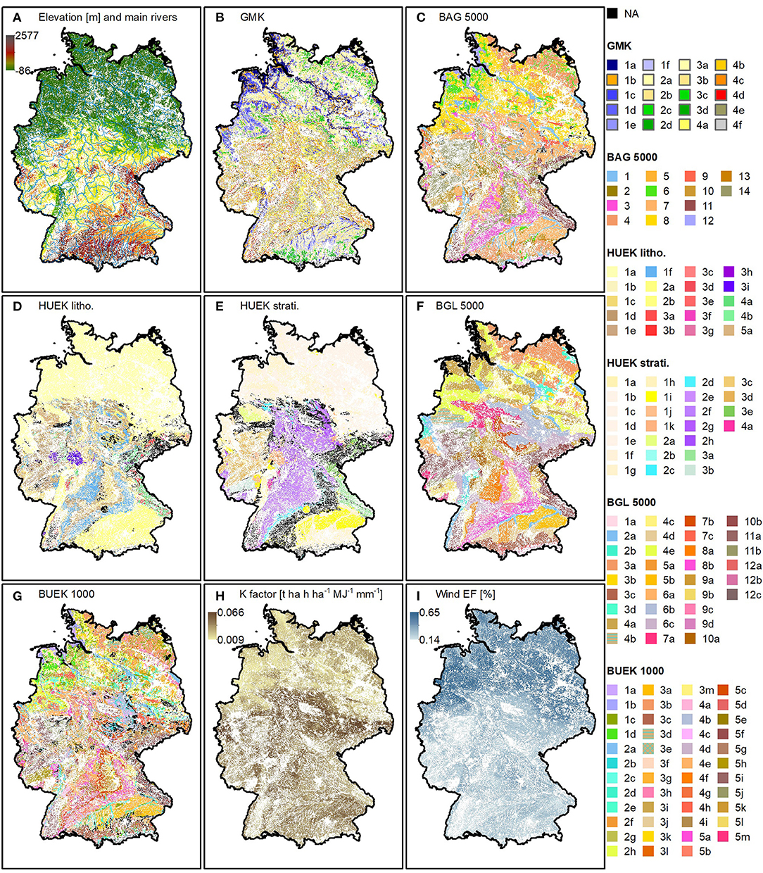
Figure 1. Selected predictor variables. (A) elevation above sea level [© (62)] and main rivers [© (63)], (B) geomorphic map of Germany (GMK) (64) [legend], (C) soil parent material map (BAG 5000) (65) [legend], (D) lithology information (HUEK litho), and (E) stratigraphy information (HUEK strati.) from the hydrological map of Germany (66) [legend], (F) soil scapes map (BGL 5000) (67) [legend], (G) soil information from the soil map of Germany (BUEK 1000) (68) [legend], (H) stone corrected K factor (69, 70), (I) wind erodible fraction (EF) (69, 71). Artificial surfaces, forests, semi natural areas, and water bodies were masked based on the CORINE land cover map [© (61)]. For the classes of the categorical predictors that are described not only with numbers but also with letters, the following applies: the number describes a category to which the classes can be summarized, the letter distinguishes the individual classes of a category. Classes of categorical predictors that were excluded from model development are shown in black.

Relief

The relief of Germany was approximated by 21 quantitative and one categorical predictor. The quantitative predictors mostly relate to water movement and erosion processes, which are known to affect particle sorting (75). Elevation and slope influence the erosion intensity; different landforms control how surface water and eroded soil material move over the landscape and where they accumulate (10). The catchment area allows identifying areas with high surface and subsurface runoff, while the SAGA topographic wetness index allows identifying areas with high soil moisture (76). They are expected to relate to lateral and vertical transport processes. Additionally, overland flow distances to the seas and the main rivers were calculated, since most rivers no longer follow their natural topographical streambeds.

The quantitative predictors were derived from the remotely sensed and quality-checked EU-DEM [(77) © (62)]. The EU-DEM is offered in 25 m resolution. It is visualized in Figure 1A. We pre-processed the EU-DEM to obtain reliable hydrology related relief predictors (catchment areas, wetness index, flow distances): sinks of more than 1 m depth were filled using the spatial analyst extension in ArcGIS (78), the main rivers were burnt into the DEM using the SAGA GIS (73) preprocessing library (74). We extracted the main rivers from the CCM river and catchment database [© (63, 79)]. They are visualized in Figure 1A. Except for the overland flow distances, the quantitative relief predictors were calculated by applying morphometry and hydrology terrain analysis tools of the SAGA GIS (73) software (74). Aspect, slope, and terrain surface convexity were calculated with three search radii (2, 4, and 8 km) to capture processes on different scales. The circular variable aspect was split into North/South and East/West direction. Overland flow distances to the center of the main rivers were calculated by applying the D-Infinity method from the spatial analyst extension in ArcGIS (78).

The only relief related categorical predictor is the geomorphic map of Germany (GMK) (64). The original map distinguishes 25 landform classes that belong to five categories (Figure 1B): sink areas (category 1), the North German lowland (category 2), the Alpine foothills (category 3), the highland (category 4), and the Alps (not represented).

Spatial Position

The X and Y coordinates were added to the predictor dataset to represent the spatial position. Adding them early in the iterative process, allows the tree models to distinguish the influence of different predictors depending on the spatial position. For example, it can be assumed that the topographic predictors play a more important role in southern Germany than in the comparatively flat northern Germany.

Organisms

The scorpan O was approximated by 15 quantitative and one categorical predictor. The quantitative predictors relate to vegetation, whose condition depends, amongst other factors, on the available water (80). The root-zone plant-available water in turn depends on the soil texture (2). The quantitative predictors comprise three spectral vegetation indices. The normalized difference vegetation index (NDVI) is highly correlated to the green biomass and therefore to the vegetation condition (81). The normalized difference red edge (NDRE) index is very similar to the NDVI but allows the evaluation of later growth stages (82). The normalized difference water index (NDWI) is directly related to the liquid water contents of the vegetation (83).

We obtained yearly temporal statistics (minimum and maximum) of NDRE, NDVI, and NDWI from the European Data Portal (84). The indices are based on remotely sensed and processed Sentinel 2 images in 10 m resolution. The maximum indices of a relatively wet year (2016) and the minimum indices of a relatively dry year (2018) were integrated into the predictor dataset. In addition, we calculated the difference (maximum–minimum) within each of the 2 years and between 2016 and 2018.

According to Jacobs et al. (57) land use depends on soil texture. We derived categorical land use data from the CORINE land cover map. It offers classified satellite data in 100 m resolution. In Europe, it distinguishes 44 classes.

Climate

The influence of the climate was included in the predictor dataset by three quantitative variables: long-term averages of precipitation and temperature in 2 m height and wind speed in 10 m height. Precipitation and temperature influence the chemical and physical weathering processes which in turn can result in different particle sizes (2). In addition, precipitation provides the input for water erosion. Wind speed is directly related to wind erosion.

Three gridded precipitation datasets (85–87) and three gridded temperature datasets (88–90) were obtained from the climate data center (CDC) of the national meteorological service of Germany (DWD). The multi-annual datasets with 1 km resolution are based on quality-checked meteorological observations that were interpolated using the elevation data (91). We summarized the three interpolations by calculating the long-term (1961–2010) means of precipitation and temperature. Gridded wind speed data in 200 m resolution was also obtained from the CDC (92). It was modeled from quality-checked meteorological observations (93).

Parent Material

The soil parent material strongly influences soil texture. Its composition is known to control the resistance to weathering (94). Depending on the stage of development, the texture of a soil resembles the texture of its parent material (95). We approximated the scorpan P by adding three polygon-based maps to the predictor dataset. The original soil parent material (BAG 5000) map at scale 1:5,000,000 (65) distinguishes 18 classes. The BAG 5000 classes that were included into model development are shown in Figure 1C. The hydrological map of Germany describes the properties of the uppermost aquifers at scale 1:250,000 (66). We extracted information on lithology (HUEK litho.) and stratigraphy (HUEK strati.). The original lithology map distinguishes 80 classes, which belong to five categories (Figure 1D): sedimentary materials (category 1), unconsolidated materials (category 2), igneous materials (category 3), composite genesis materials (category 4), and other materials (category 5). The original stratigraphy map distinguishes 97 classes, which belong to four categories (Figures 1E,F): the Cenozoic period (category 1), the Mesozoic period (category 2), the Paleozoic period (category 3) as well as the Precambrian (category 4).

Soil

Soil can be predicted from other soil attributes (13). We included two polygon-based soil maps and two grid-based erosion maps into the predictor dataset. The soil scapes (BGL 5000) polygon map at scale 1:5,000,000 aggregates similar soil typological units (67). The original map comprises 38 classes that belong to 12 soil regions (Figure 1F): coastal Holocene (category 1), river landscapes (category 2), young and old moraine landscapes (categories 3 and 4), gravel plates and tertiary hills in the Alpine foothills (category 5), loess and sand loess landscapes (category 6), mountainous and hilly areas with different non-metamorphic rocks (categories 7, 8, and 9), or with many magmatites and metamorphic rocks (category 10), or with many clay and silt slates (category 11), and the Alps (category 12). Polygon-based soil information was extracted from the land use-stratified soil map (BUEK 1000) of Germany at scale 1:1,000,000 (68). The original map distinguishes 72 classes that are grouped into soils of the coastal area and peat soils (category 1), soils of broad river valleys, (category 2), soils of the undulating lowlands and hilly areas (category 3), soils in loess areas (category 4), soils of the mountain and hilly regions as well as of the low mountain ranges (category 5), and soils of the high mountains, anthrosols, settlements and surface water (not represented) (Figure 1G). Two erosion maps were obtained from the European soil data center (69). The K factor map (Figure 1G) in 500 m resolution describes the soil erodibility taking into account the stoniness. It was generated for Europe by applying a cubist model to extract the relationship between K factor point data from the European soil database and the LUCAS point survey, and spatial predictors (70). The wind erodible fraction (EF) map (Figure 1H) in 500 m resolution is directly related to the soil wind erosion susceptibility. Similar to the K factor, it was created by applying a cubist model to extract the relationship between wind EF point data from the LUCAS survey, and spatial predictors (71).

Model Development and Evaluation

Model development and statistical analysis were done using the R language (96). We applied the boosted regression trees (BRT) algorithm for model development because it can use categorical and quantitative predictors without preprocessing, it considers predictor interaction, and it is robust to irrelevant predictors, predictors with missing data as well as overfitting (97). We trained and applied BRT models using the “gbm” R-package (98). For a detailed explanation of the BRT algorithm, please refer to the publications of Elith et al. (97) and Ridgeway (99). Briefly, the BRT algorithm combines two machine learning techniques: regression trees and stochastic gradient boosting. Regression trees recursively divide the response variable data into increasingly similar subgroups. All predictor variables are compared to find the best decision rule for each binary split. Finally, the response variable values of the terminal regression tree nodes are averaged per subgroup. Boosting combines many simple models to form a linear combination. The BRT algorithm fits simple regression trees to random training data subsets and adds them iteratively. To improve the overall model accuracy, new trees are trained to reduce the residuals of the previous trees. The “gbm” R-package includes a function to calculate the relative importance of each predictor variable. The importance depends on how often the respective predictor was used to divide the response variable data into BRT subgroups, and how much its usage improved model performance (100).

Two continuous and three discrete valued model parameters were tuned to adapt the BRT algorithm: the number of simple regression trees to be combined (n.trees, discrete), the contribution of each tree to the final model (shrinkage, continuous), the number of splits to divide the data (interaction.depth, discrete), the fraction to subset the response variable dataset randomly (bag.fraction, continuous), and the minimum number of observations in the terminal tree nodes (n.minobsinnode, discrete). We applied the differential evolution algorithm for parameter tuning using the R-package “DEoptim” (101). For a detailed explanation of the differential evolution algorithm, we refer to the book of Price et al. (102). Briefly, the differential evolution algorithm is based on evolutionary theory. It consists of the steps mutation, crossover, and selection that are repeatedly applied to a population. The fitness of the population is optimized by minimizing an objective function. In this study, each member of the population is reflected by a vector of five elements. Each vector element represented the value of one tuning parameter. During optimization, the differential evolution algorithm allows any real tuning parameter value between two user-defined limits. To choose these limits, we extended the recommendations of Elith et al. (97) and Ridgeway (99) to accommodate the complex dataset used in our study. The chosen limits are summarized in Table 2. Besides that, the differential evolution algorithm was applied in the same way as described in Gebauer et al. (41): a population consisted of 100 members, the root mean squared error (RMSE) was used as objective function value, and optimization was either stopped after 200 repetitions or after the 10th repetition without any RMSE improvement.

TABLE 2

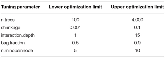
Table 2. Tuning parameter limits that are required for optimization by differential evolution.

To ensure independent test and training datasets for a reliable model performance evaluation, we applied k-fold cross-validation (CV) for two purposes. First, to calculate the objective function during parameter tuning, and second to evaluate the final models with optimized parameter values using two common error metrics: RMSE and the coefficient of determination (R²). To combine both purposes, we used a nested CV approach similar to Guio Blanco et al. (103). During k-fold cross-validation the dataset is divided into k folds; k−1 folds form the training dataset, one-fold forms the test dataset. Model training and evaluation are repeated k times until each fold is used as a test set once. To include parameter tuning, an inner parameter tuning CV loop is nested in an outer final model evaluation CV loop. For this purpose, the training folds of the outer loop form the total dataset for the inner loop. The dataset of the inner loop is divided into test and training folds, to compare the performance of models with different tuning parameter values. We used k = 5 fold CV with one repetition for parameter tuning and with five repetitions for model evaluation.

To guarantee that each fold is representative of the whole dataset, we divided the datasets pseudo-randomly using spatial stratification. In addition, this ensured the direct comparability of all models, since the clay, silt, and sand response variable datasets were divided into test and training folds in the same way. First, Germany was divided into 50 strata based on a 100 × 100 km raster. For this, we used the INSPIRE-compliant grid generation tool (72). Second, these strata were sampled randomly and data was distributed into the folds. Spatially autocorrelated training and test data, which could cause overly optimistic error metrics, can be precluded because of large distances between neighboring sampling points: on average the distance is 8,120 m; for <0.02% of the sampling points the distance is between 1,400 and 7,900 m.

Results and Discussion

Response Data and Predictor Representation

The topsoil clay, silt, and sand data are visualized by maps in Figure 2.1, and by boxplots and violin plots in Figure 2.2. Most of the sampled topsoils contain less clay than silt and sand. The median clay content is 15.9 wt.%, the median silt content is 35.4 wt.%, and the median sand content is 41.6 wt.%. Overall, the sand contents cover the widest range. They vary between 0.8 and 97.1 wt.%, while silt contents range between 1.7 and 86.5 wt.%, and clay contents between 1.0 and 77.7 wt.%. Most of the high clay and silt contents were measured in southern Germany, most of the high sand contents in northern Germany.

FIGURE 2

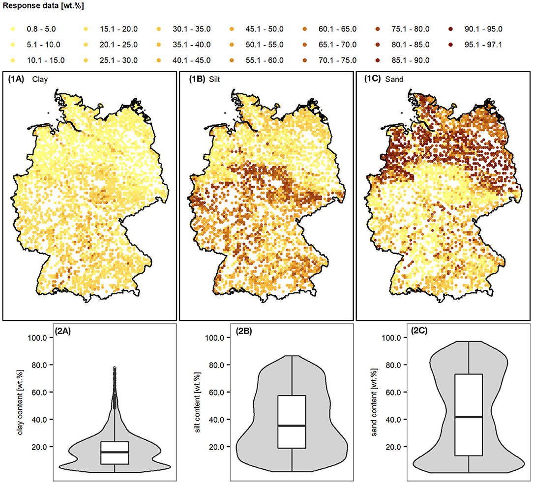
Figure 2. Response variable datasets. Data was obtained from the harmonized database of the first German agricultural soil inventory (56). 2.1 location and 2.2 data distribution of the topsoil (A) clay, (B) silt, and (C) sand contents.

The high quality of the first German agricultural soil inventory data and its representativeness for mineral soils under croplands and grassland has already been confirmed by Jacobs et al. (57). The plots in Figure 2.2 reveal that the extracted response datasets cover a wide range of texture values very well. Only some comparatively high clay contents (>48.0 wt.%) are rare. Most of the high clay contents belong to soil profiles that are located comparatively close to the main rivers. Their median horizontal overland flow distance to the center of the closest main river is 5,400 m. The median distance of the other soil profiles is 8,500 m.

Not only the response data influences the model performance but also the predictor data. The better the spatial predictors are represented by the predictor values at the sampling points of each CV test and training dataset, the more information can be used by the model and the more stable the spatial predictions. Therefore, we compared the predictor subspace of each CV fold of the outer loop to the complete spatial predictor space under agricultural land use. The large difference in the size of the two datasets did not allow to perform a robust statistical test. For each quantitative predictor, we compared the medians and interquartile ranges of both datasets instead. The results of the comparisons are similar for each CV fold because the spatial stratification resulted in similar predictor subspaces per fold (section Model Development and Evaluation). Consequently, we averaged the differences in medians and interquartile ranges per quantitative predictor across all 25-folds resulting from five-fold CV with five repetitions. The comparison shows that the spatial predictor space under agricultural land use can be represented by our test and training datasets. For almost all quantitative predictors, the averaged difference of the medians of the two data sets ranges only between 0.1% [X and Y coordinates, terrain surface convexity (8 km search radius)] and 9.4% (range NDRE 2016). For half of the quantitative predictors, the difference is <3%. The only exception is the SAGA catchment area; the average difference of the medians is 23.9%. The interquartile ranges of the two data sets differ more than the medians. Predictors at sampling sites cover a smaller interquartile range than the spatial predictors. The averaged difference of the interquartile ranges of the two data sets varies between 0.3% [North/South direction of the aspect (4 km search radius)] and 44.3 % (minimum NDVI 2018). For half of the quantitative predictors, the difference is higher than 9.5%. Comparatively large differences in the interquartile ranges occur because small areas with extreme quantitative predictor values are unlikely to be represented by the soil survey sites. These are mainly areas in the Alps with elevations of more than 1,100 m above sea level (a.s.l.). They cover only 1.2% of the area of agricultural soils.

We excluded classes of categorical predictors from model development that were not included in each CV fold of the outer loop at least once. Except for the CLC land cover predictor, the excluded categorical classes are visualized as black areas in Figure 1. As indicated by Jacobs et al. (57), only small areas are not covered sufficiently by the sampling sites of the agricultural soil inventory. The excluded predictor classes cover only 1.1% (5 GMK classes), 4.3% (8 agricultural CLC classes that occur in Germany), 0.1% (4 BAG 5000 classes), 6.1% (60 HUEK litho. classes), 13.0% (72 HUEK strati. classes), 1.8% (5 BGL 5000 classes), and 6.2% (25 BUEK 1000 classes) of the area of agricultural soils. This leaves 20 GMK classes, 3 CLC classes, 14 BAG 5000 classes, 20 HUEK litho. classes, 25 HUEK strati. classes, 33 BGL 5000 classes, and 47 BUEK 1000 classes forming the categorical predictor input. Most of them are well represented. Only 20 classes occur <25 times in the model input (i.e., on average five times per fold): GMK classes 3c and 3d, CLC vineyards, HUEK strati. classes 1c, 1j, 2b, 3c, and 4a, BGL 5000 class 6b, and BUEK 1000 classes 1a, 2b, 2c, 2f, 4a, 4c, 4f, 4g, 5g, 5h, and 5j (class labels refer to the legend in Figure 1). They cover only 1.5% (GMK), 0.6% (CLC), 3.4% (HUEK strati.), 5.9% (BGL 5000), and 7.7% (BUEK 1000) of the area of agricultural soils.

Predictor Importance

The relative importance of each predictor per iterative step of the silt models is shown in Figure 3 by boxplots. While considering only scorpan R (iterative approach, step 1), elevation is by far the most important predictor (Figure 3A). Its median relative importance among all predictors of scorpan R is 41%. This is not surprising as the elevation is already related to other scorpan factors. It for example relates to the climate and allows to divide Germany into 5 major landscapes (104): the glacially shaped North German lowlands with elevations mostly below 100 m a.s.l. (dark green areas, Figure 1A), the adjacent low mountain ranges with elevations up to ~1,000 m a.s.l. (mostly yellow, orange, and red areas, Figure 1A), the Upper Rhine valley with elevations around 150 m a.s.l. (mostly light green areas, Figure 1A), the Alpine foothills with elevations between ~500 and 750 m a.s.l. (orange and red areas, Figure 1A), and the Alps with elevations of more than ~1,100 m a.s.l. (gray areas, Figure 1A). To some extent, the landscapes differ in their parent materials (compare e.g., Figures 1A,D) and their susceptibility to wind and water erosion (compare Figures 1A,H,I). While the potential relief energy in the North German lowlands, the Upper Rhine valley, and the Alpine foothills is comparatively low, the steep slopes in the low mountain ranges and the Alps are much more susceptible to topography-induced mass movements (105, 106). The second most important relief predictor is the geomorphic map of Germany (GMK). Its median relative importance is 10%. It adds important information to the predictor space by classifying the landscapes into different landforms. In addition, it is related to the parent material and the soil distribution (compare e.g., Figures 1B,C,G). Another important scorpan R predictor is the multi resolutional index of valley bottom flatness (MRVBF). It allows identifying depositional areas (107), which explains its comparatively high median relative importance of 6%. Its relevance for texture predictions was also reported by studies conducted in Iran (26, 35), Denmark (21), and Europe (54). We assume that, together with the elevation and the GMK map, it covers most topography-driven transport processes. This explains the comparatively low importance of the other relief related predictors. Their median relative importance is <5%.

FIGURE 3

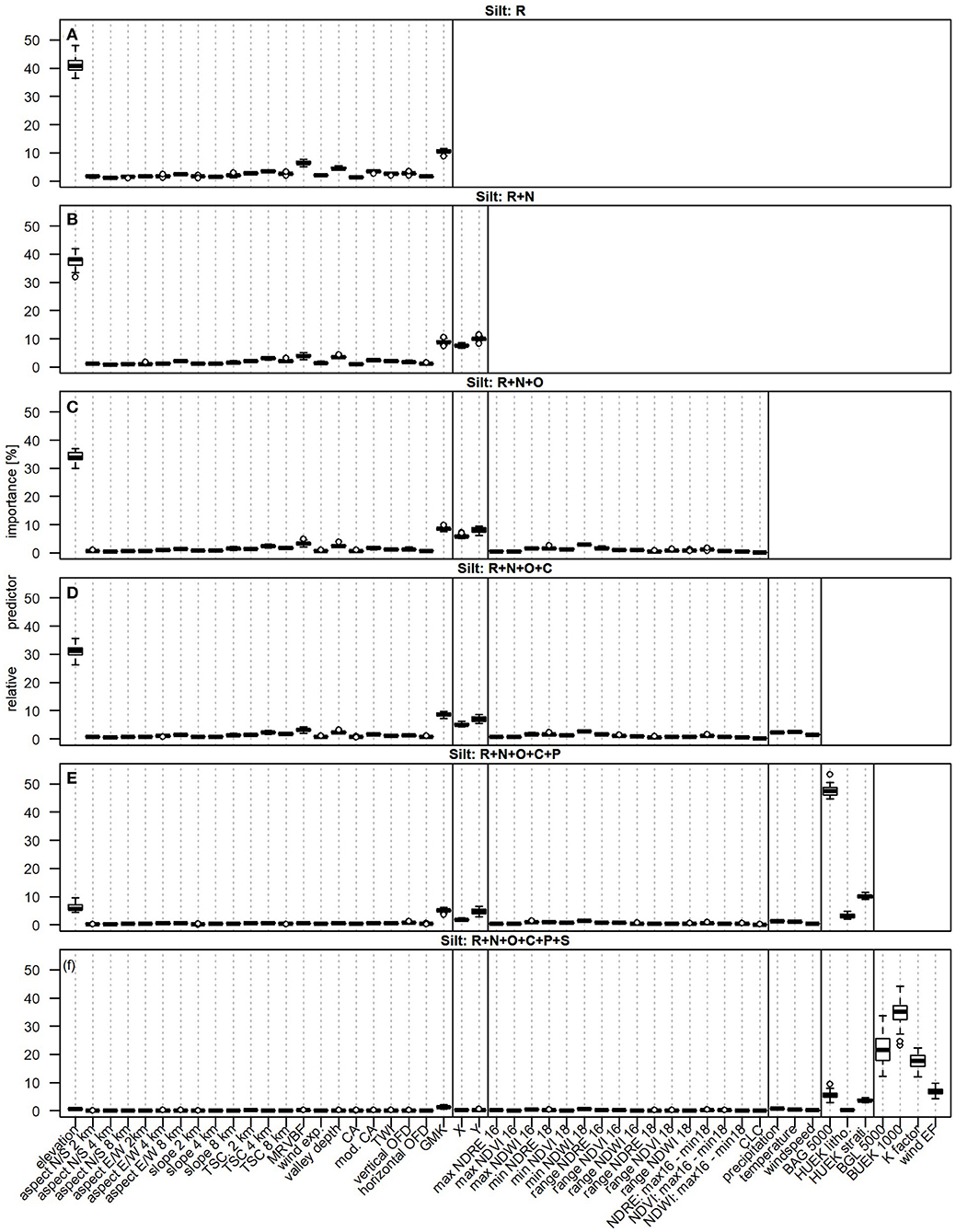
Figure 3. Boxplots comparing the relative predictor importance of the iterative approach (silt models). Variables that approximate six scorpan factors were added iteratively to the predictor dataset: (A) relief (R), (B) spatial position (R+N), (C) organisms and land use (R+N+O), (D) climate (R+N+O+C), (E) parent material (R+N+O+C+P), and (F) other soil properties (R+N+O+C+P+S). Predictor abbreviations are explained in Table 1. Gray, dotted lines are used for orientation; solid, black lines separate the scorpan factors. Each boxplot is based on 25 values resulting from five-fold CV with five repetitions.

Adding the spatial position to the predictor dataset (scorpan R+N, Figure 3B) decreases the relative importance of the relief predictors. Instead, the X and Y coordinates account for about 8 and 10% of the relative importance. Together with the elevation and the geomorphic map of Germany (GMK), they are among the predictors with a median relative importance of more than 5%. The comparatively high importance of the coordinates indicates that factors influencing the spatial texture distribution are still missing in the predictor data set (13). It is not surprising that the relief predictors alone are not able to explain the soil texture distribution completely. Similar findings were made when predicting the soil texture in Denmark (30) and a small area in East Germany (108). In addition, the Y coordinates can be used to partially distinguish the sandy deposits (HUEK litho. class 1a, Figure 1D) in the north from the other parent materials.

Adding the organisms predictors barely causes any changes (scorpan R+N+O, Figure 3C). The minimum NDWI 2018 is the most important scorpan O related predictor. Still, its median relative importance is only 3%. We believe that the BRT models were not able to effectively learn from the vegetation indices because of three reasons. First, due to the large research area and satellite data as composite of many scenes recorded during 1 year, the vegetation indices refer to different plant species of different growing stages. Second, Reinermann et al. (109) were able to show that the impact of the 2018 drought in Germany depended on the crop type. Third, the plant condition on German agricultural soils does not only depend on soil texture but also for example on climate, on diseases and pests, fertilization, and irrigation. This is known to complicate deriving useful predictors from spectral images (110). Even though, the soil texture differs between grassland and croplands (57), the CORINE land cover map (CLC) has a rather low importance. The reason for this is probably its rather low information content compared to the other predictors: the CLC map only allowed to distinguish between three land use classes, with 94% of the sampled soil profiles already classified as grasslands or croplands. The low importance corresponds to the results of Ballabio et al. (54). Even though their continental-scale study area (Europe) allowed to incorporate 44 CLC classes, the land cover map was not among the 38 most important predictors.

Adding the climate predictors causes only a few changes (scorpan R+N+O+C, Figure 3D). The most important climate predictor is the long-term average temperature. Its median relative importance is only 2%. We assume that the scorpan C predictors are comparatively unimportant as they are substituted by the scorpan R and N predictors, which were available at higher resolution. Air temperature and precipitation are for example influenced by the increasing continentality from northwest to southeast and depend on the elevation (111–113). Besides, both datasets are based on meteorological observations that were interpolated using the elevation data (section climate). The relief influences also the wind: in the flat coastal regions it is usually very windy, while the mountains in the south slow down the wind speed (114). In general, the used scorpan C predictors can maximally reflect the Holocene climate up to the end of the Weichselian ice age about 10,000 years ago (115). Our results contrast those of Ballabio et al. (54), who rated precipitation and temperature as very important even though they also used scorpan R variables. Therefore, we assume that scorpan C predictors have a more significant influence on the texture distribution at larger scales due to their higher range. In general, the results depend on the iterative order.

Adding the parent material related predictors (scorpan R+N+O+C+P, Figure 3E) remarkably changes the relative importance of the previous predictors. Now, the by far most important predictor is no longer the elevation, but the soil parent material map (BAG 5000). Its median relative importance is 47%. The second most important predictor is the stratigraphy information from the hydrological map of Germany (HUEK strati.). Its median relative importance is 10%. The elevation accounts for about 6% of the relative importance and the geomorphic map of Germany (GMK) for about 5%. The median relative importance of the other predictors is <5%. According to the review of Zhang et al. (15), missing parent material information is one of the main reasons for poor predictive soil mapping results. If it is available, it is almost always one of the most important predictors of soil texture. This is confirmed, for example, by the results of three studies that focused on the soil texture predictions in Denmark (30), the French metropolitan territory (50), and New South Wales (Australia) (22). In Germany, we are in the fortunate situation that several maps with information on the parent material were available. We assume that the BAG 5000 map is much more important than the HUEK litho. and HUEK strati. maps because of two reasons. First, its classes can be better represented by the predictors at sampling sites than the HUEK litho. and HUEK strati. classes (section Response Data and Predictor Representation). Second, the BAG 5000 map provides detailed information on the soil parent material, while the HUEK maps focus on the geology of the uppermost aquifers. The BAG 5000 map distinguishes for example floodplain sediments, sands and thick sandy cover layers, as well as intertidal sediments in the North German lowlands (classes 1, 8, 12, Figure 1C), while the HUEK litho. map assigns most of the North German lowlands to sand (class 1a, Figure 1D). The HUEK strati. map assigns the North German lowlands mostly to the Saalian, Weichsalian, and Ionian ages (classes 1d, 1e, 1g, Figure 1E). This slightly more detailed subdivision might explain why it is more important than the HUEK litho. map.

Adding the scorpan S variables to the predictor dataset (scorpan R+N+O+C+P+S, Figure 3F) also led to major changes. The four variables that were assigned to the scorpan S factor, are the most important predictors in step six. Their median relative importances are 32% (BUEK 1000), 25% (BGL 5000), 16% (K factor), and 7% (wind EF). The soil parent material map (BAG 5000) now accounts for about 5% of the relative importance. The median relative importance of the other predictors is <5%. Our results correspond to those of Adhikari et al. (21), who emphasize the importance of soil maps when predicting the soil texture of Denmark. The main reason for the high importance of the scorpan S predictors in our study is that they can partly substitute the predictors of the previous step. A phenomenon in predictive soil mapping that was also described by Miller et al. (108). Soil development in Germany depends a lot on relief and parent material (116, 117). The soil map (BUEK 1000) was derived on behalf of relief and parent material information. Not only the BUEK 1000 but also the soil scapes (BGL 5000) map reflect the scorpan R and P predictors (compare Figures 1B,C,F,G). The soil erodibility (K factor) and the wind erodible fraction (wind EF) were, among others, derived on behalf of elevation data (93, 94; compare Figures 1A,H,I). Overall, the low relative predictor importance of the X and Y coordinates, which is much below 1%, indicates that the predictor dataset of the last iteration covers almost all factors influencing the silt distribution in Germany.

As expected, the influence of the predictors for the clay, silt, and clay models is similar. Predictor variables of the clay and sand models that account for at least 1% of the relative importance are compared to those of the silt models in Figure 4. Similar to the silt models, the scorpan S predictors play an important role when predicting the clay and sand distribution. The soil map (BUEK 1000) accounts for about 15% (clay) and 23% (sand) of the relative predictor importance, the soil scapes map (BGL 5000) for about 21% (clay) and 9% (sand). Erosion influences not only the silt distribution but also the clay and sand distribution. However, the influence of the K factor and the wind EF in the clay and sand models differs from that in the silt models. The most important predictor of the clay and sand models is the wind EF. Its median relative importance is 31% (clay) and 39% (sand). While the wind EF plays a more important role in predicting the clay and sand distribution than the K factor, which accounts for about 1% (clay) and 6% (sand), the reverse is true for silt. It remains difficult to interpret why the predictor importance of K factor and wind EF differs. The correlation between both predictors (Spearman's rho: −0.63^****) would suggest that they influence all three texture classes. Similar to the silt models, the most important scorpan P predictors in the clay and sand models are the soil parent material map (BAG 5000) and the stratigraphy information from the hydrological map of Germany (HUEK strati.). The BAG 5000 map accounts for 2% (clay) and 7% (sand) of the relative importance, the HUEK strati. map for 7% (clay) and 4% (sand). The median relative predictor importance of the elevation, the geomorphic map of Germany (GMK), and the lithology information from the hydrological map of Germany (HUEK litho.) is <5%; in the case of the silt and sand models, partly even <1% (elevation, HUEK litho). Similar to the silt models, the relative importance of the X and Y coordinates is much below 1%, which indicates that the overall predictor dataset covers almost all factors influencing the clay and sand distribution in Germany.

FIGURE 4

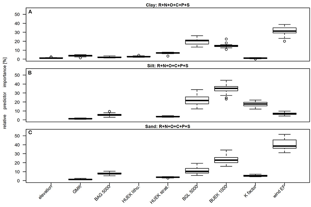
Figure 4. Boxplots comparing the relative importance of the most important predictors. (A) Clay, (B) silt, and (C) sand models. Only predictors that account for at least 1% of the relative importance are shown. Models were trained on predictors approximating the scorpan factors R, N, O, C, P, and S. Predictor abbreviations are explained in Table 1. Each boxplot is based on 25 values resulting from five-fold CV with five repetitions.

Model Performance

The predictive model performance is visualized by R² and RMSE values in Figure 5. The error metrics are compared to the results of Ballabio et al. (54) and Hengl et al. (55). Their results were evaluated using our test datasets to allow for a direct comparison.

FIGURE 5

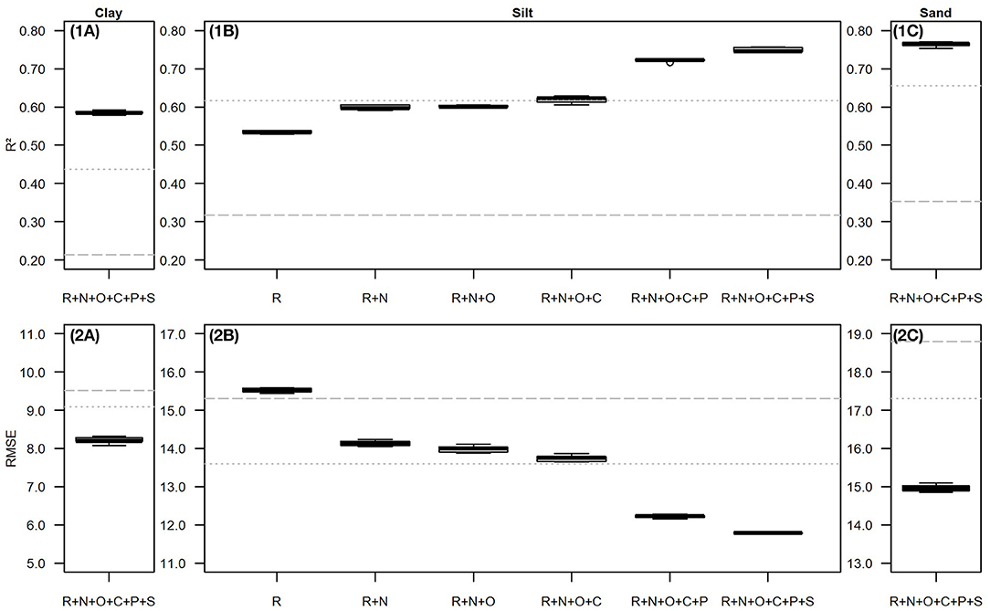
Figure 5. Boxplots comparing the model performance. (A) Clay, (B) silt, and (C) sand models. (5.1) Root mean squared error (RMSE) and (5.2) coefficient of determination (R²). Models were trained on predictors approximating the scorpan factors R, N, O, C, P, and S. Each boxplot is based on 25 values resulting from five-fold CV with five repetitions. The dotted gray lines refer to the publication of Ballabio et al. (54), who predicted the topsoil (0–20 cm) texture of Europe. The dashed gray lines refer to the publication of Hengl et al. (55), who predicted soil texture in 30 cm depth on global scale. Both publications used USDA texture class limits: clay (<2 μm), silt (2–50 μm), and sand (50–2,000 μm). We followed Shang (118) and used spline interpolation to convert their predictions to the texture class limits used in this study. The predictions of Ballabio et al. (54) and Hengl et al. (55) were evaluated using our test datasets to allow for a direct comparison. Please note the different axis labels in 5.2 (RMSE).

Even though the results of the iterative approach (Figure 5B) depend on the iterative order, they allow detailed insights into model interpretation. They confirm the results described in section Predictor Importance; certain predictor variables can substitute others to some extent: The scorpan R predictors and their interactions are related to other scorpan factors. They are assumed to cover most topography driven transport processes. Therefore, BRT models trained only on scorpan R predictors already explain about 53% of the silt variance; their median RMSE is 15.5 wt.%. Nevertheless, important predictor information is still missing which is why adding the spatial position to the predictor dataset improves model performance by about 11% (median R²) and 10% (median RMSE). The scorpan O and C predictors seem to barely improve the model performance. However, this might look different if the spatial position would have been excluded. R² values of the respective silt models range between 0.60 (R+N+O) and 0.63 (R+N+O+C); RMSE values range between 13.6 wt.% (R+N+O+C) and 14.1 wt.% (R+N+O). In correspondence to their high relative importance, adding the scorpan P predictors to the dataset improves model performance by about 14% (median R²) and 12% (median RMSE). Despite their high relative importance, the scorpan S predictors cause comparatively little additional improvement. Median R² and median RMSE improved by only 4%. As explained in section Predictor Importance, this is because the scorpan S predictors rather substitute other predictors, than provide additional information: the BUEK 1000 soil map, for example, was derived on behalf of relief and parent material information, the two soil erosion maps, among others, on behalf of elevation data. Still, the best results are achieved by training the BRT clay (Figure 5A), silt (Figure 5B), and sand (Figure 5C) models on the complete predictor dataset. Altogether, the interaction of 50 predictor variables enabled the BRT models to explain about 59% of the clay variance, 75% of the silt variance, and 77% of the sand variance. Their median RMSE values are 8.2 wt.% (clay), 11.8 wt.% (silt), and 15.0 wt.% (sand).

It is not surprising that our results differ from those of Ballabio et al. (54) and Hengl et al. (55) as their models were not developed for agricultural soils in Germany specifically, but for continental (Europe) and global scales. Our silt models that were trained on scorpan R and N predictors already resulted in lower RMSE and higher R² values than those derived from the predictions of Hengl et al. (55). While we obtained the response variable datasets from one national soil inventory, Hengl et al. (55) had to harmonize different data sources due to the larger research area. Adding scorpan P predictors to the dataset resulted in lower RMSE and higher R² values than those derived from the predictions of Ballabio et al. (54). While we used three scorpan P predictors, Ballabio et al. (54) did not incorporate variables that are directly related to the parent material. It is difficult to compare our results to further texture predictions due to differences in the research area characteristics, the model algorithms, and most importantly, the input data. For texture predictions in particular, missing scorpan P information is critical. The topsoil texture predictions of Gray et al. (22), Greve et al. (30), and Wadoux (50) are roughly comparable to ours. In Denmark, Greve et al. (30) trained regression tree models on response variable datasets sampled in 7 km intervals and on predictor variables representing the scorpan factors S, C, R, and P. The resulting models explained between 52% (fine sand) and 60% (clay, silt) of the response variable variance. Wadoux (50) trained a convolutional neural network to predict the topsoil texture in the French metropolitan territory. His response variable data was obtained from the LUCAS topsoil database and the predictor variables represented all scorpan factors. However, the resulting R² values ranged only between 0.22 (clay) and 0.40 (silt). Gray et al. (22) predicted the clay distribution in New South Wales (Australia). Their random forest model was able to explain 57% of the clay variance after being trained on more than 2,600 point values as well as a predictor dataset approximating scorpan C, O, R, and P factors.

Although our error metrics are comparatively good, some texture values are difficult to reproduce. The scatterplots in Figure 6 were drawn to identify high absolute deviations between measured and predicted clay, silt, and sand contents. Predictive uncertainties occur over the entire range of texture values. Overall, the mean is unbiased for clay, silt, and sand. However, it is particularly noticeable that high absolute deviations from the measured values occur when predicting high clay contents (>48.0 wt.%) and medium sand contents (30.0–60.0 wt.%). The median predictions of the high clay contents are up to approximately 52 wt.% too low. These comparatively high deviations can be attributed to the distribution of the respective response variable: high clay contents are rather rare (Figure 2.2). The medium sand contents are both, overpredicted (up to 51.4 wt.%) and underpredicted (up to 44.1 wt.%). Approximately 22.0% of them belong to soils that developed from boulder clay (BAG class 4, Figure 1C). For comparison, only 7.5% of the other soil profiles were assigned to this class.

FIGURE 6

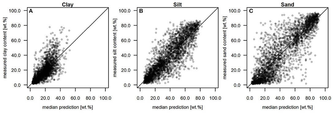
Figure 6. Scatterplots comparing the measured and the predicted texture values. (A) Clay, (B) silt, and (C) sand contents. Models were trained on predictors approximating the scorpan factors R, N, O, C, P, and S. Each point represents the median of 25 predictions resulting from five-fold CV with five repetitions.

Calculating the relative residuals by dividing the median absolute residuals by the measured texture values allows a more differentiated analysis. The relative residuals of models that have been trained on the complete predictor dataset are mapped in Figure 7. The relative clay and silt residuals are relatively similar; they range between −0.8 and 7.5 (clay), and −0.7 and 12.4 (silt). The relative sand residuals are higher; they range between −0.9 and 45.8. Even though some relative residuals are particularly high, the BRT models can reproduce most values well. Approximately 76% (clay), 81% (silt), and 69% (sand) of the relative residuals range between −0.5 and 0.5; ~20% (clay), 28% (silt), and 31% (sand) range between −0.1 and 0.1. Relative residuals that range between 0.1 and 0.5 or −0.5 and −0.1 are uniformly distributed throughout Germany in all three texture classes. The same applies to the relative clay and silt residuals between −0.1 and 0.1. The lowest relative sand residuals (−0.1 to 0.1) concentrate in the North German lowlands. More than 71% of them belong to soil profiles with high topsoil sand contents (66.6 wt.% on average) that developed from Saalian, Weichselian, and Ionian (HUEK strati. classes 1d, 1e, and 1g, Figure 1) sand deposits (HUEK litho. class 1a, Figure 1). These predictor classes are particularly well-represented by the response variable data set, which might explain the comparatively good predictions. More than 50% of all soil profiles were assigned to at least one of the described HUEK classes. In addition, high absolute uncertainties in the predictions of the high sand contents have comparatively little effect on the relative residuals. The relative residuals show, that not only the rare high clay and medium sand contents but also some rather low values cannot be reproduced by the BRT models. Comparatively high relative clay and silt residuals (< −0.5 or more than 0.5) can be found throughout Germany, but occur slightly more frequently in the North. This is because the clay and silt contents that were measured in northern Germany were mostly low so that even small absolute prediction uncertainties could cause high relative residuals. Most of the high relative clay and silt residuals do not belong to soil profiles with specific predictor values or classes. Only seven soil profiles, which partially correspond, stand out. Their particularly low topsoil clay (2.6 wt.% on average) and silt (3.3 wt.% on average) contents cannot be reproduced at all and belong to relative residuals of more than 5. Most of these profiles are situated in sink areas of river valleys (GMK category 1, Figure 1B). The small-scale water erosion processes that determine the spatial texture pattern here could probably not be captured by our response and predictor data. Some comparatively high relative sand residuals (< −0.5 or more than 0.5) can be found in North Germany close to the coast or in the river valleys. They are probably also caused by unrepresented small-scale water erosion processes. But most of the high relative sand residuals occur in South Germany. This is because low sand contents were mainly measured in the South, where small absolute prediction uncertainties can cause high relative residuals. Additionally, ~39% of the high relative sand residuals can be explained by the fact that the respective soil profiles belong to at least one either poorly represented or excluded class of the categorical predictors (section Response Data and Predictor Representation). For comparison, this applies to only 17% of the other soil profiles. Approximately 2% of the sand measurements cannot be reproduced at all. These particularly low sand contents (3.5 wt.% on average) belong to relative residuals that are higher than 5. Most of them are located in central Germany where the parent material is highly variable.

FIGURE 7

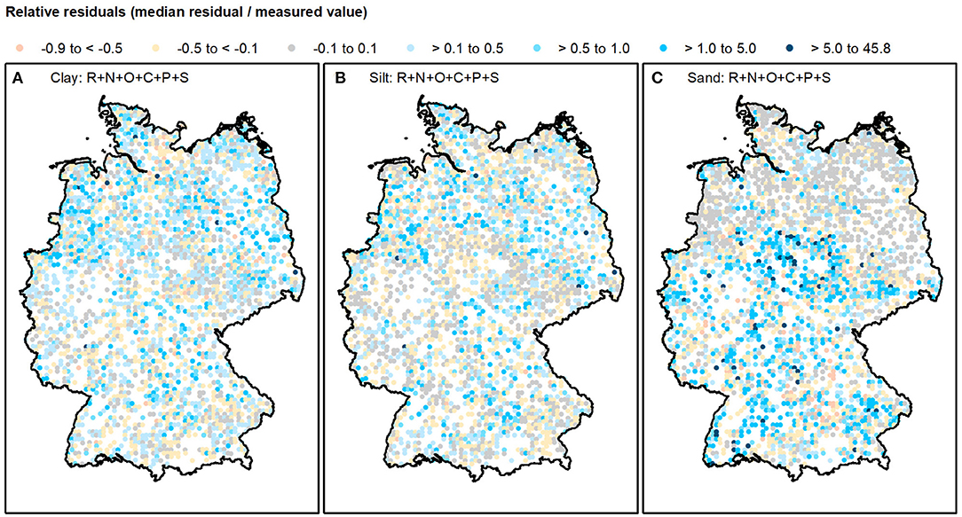
Figure 7. Maps showing the relative residuals. Relative (A) clay, (B) silt, and (C) sand residuals. Models were trained on predictors approximating the scorpan factors R, N, O, C, P, and S. The relative residuals were calculated by dividing the median residual of 25 predictions resulting from five-fold CV with five repetitions by the measured value.

Spatial Predictions

Models that were trained on the complete predictor dataset were applied to predict the spatial clay, silt, and sand content distributions for soils under agricultural land use in Germany. The median of the 25 models' predictions are visualized in Figure 8. The corresponding interquartile ranges, as a representation of the model uncertainty, are visualized in Figure 9. The median clay content predictions range between 2.8 and 64.1 wt.%, the median silt content predictions range between 3.1 and 89.2 wt.%. The median sand predictions cover the widest range. They range between 0.0 and 96.1 wt.%.

FIGURE 8

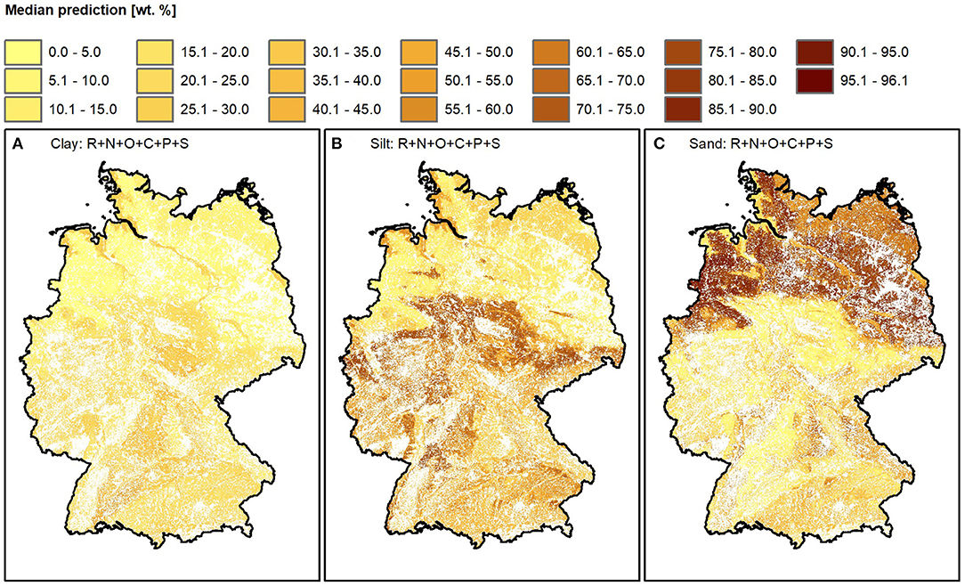
Figure 8. Maps showing the median spatial texture predictions. (A) Clay, (B) silt, and (C) sand content. Models were trained on predictors approximating the scorpan factors R, N, O, C, P, and S. Soils that are not under agricultural land use were masked. The medians were calculated from 25 predictions resulting from five-fold CV with five repetitions.

FIGURE 9

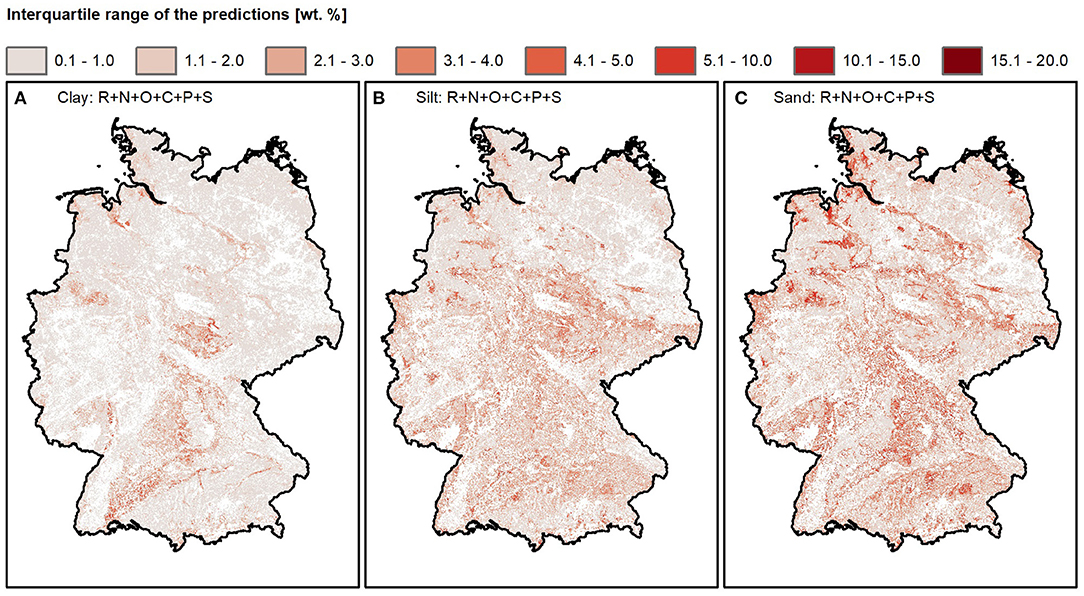
Figure 9. Maps showing the interquartile ranges of the spatial texture predictions. (A) Clay, (B) silt, and (C) sand content. Models were trained on predictors approximating the scorpan factors R, N, O, C, P, and S. Soils that are not under agricultural land use were masked. The interquartile ranges were calculated from 25 predictions resulting from five-fold CV with five repetitions.

The detailed spatial soil texture pattern mainly reflects scorpan S, P, and R predictors. In the North German lowlands, glacial deposits explain the comparatively low clay and silt contents. During the three Pleistocene ice ages, glaciers that progressed from Scandinavia reached up to today's low mountain ranges (115, 119). After melting they left mostly coarse sedimentary deposits (120). Due to the high predictive performance of the BRT models, the resulting spatial predictions can differentiate between the up to 96.1 wt.% high sand contents in the northwest and the slightly lower sand contents in the northeast. The comparatively high sand contents mainly result from sand and thick sandy cover layers (BAG 5000 class 8, Figure 1C) in old moraine landscapes (BGL 5000 category 4, Figure 1F). The last ice sheet, that progressed from the North about 20,000 years ago, extended not that far inland (115). Only in the northeast, it left a young moraine landscape (BGL 5000 category 3, Figure 1F) with boulder clay and loam partly alternating with cover layers of different thicknesses (BAG 5000 classes 4 and 5, Figure 1C). The slightly lower sand contents of these soils also show a higher erodibility (K factor, Figure 1H). The high clay and silt contents along the North Sea and those in the river valleys form a strong contrast to the high sand contents in North Germany. The tides led to the deposition of fine sediments along the North Sea coast, from which fertile marsh soils developed (BUEK 1000 classes 1a, 1b, Figure 1G) (121–123). Despite the strong wind in the coastal regions, the marsh soils have a comparatively low wind EF due to their high organic matter contents (Wind EF, Figure 1I). The flow velocity of the rivers is reduced due to the low relief energy in North Germany (105). Consequently, their fine-grained sediments are deposited mostly in depressions (GMK class 1a Figure 1B; 121). The soil parent material map classifies them as alluvial sediments (BAG 5000 classes 2, Figure 1C), the soil scapes map assigns them mostly to lowlands and glacial valleys of the young moraine area (BGL 5000 class 2a, Figure 1F), and the soil map allows to distinguish 8 soils of broad river valleys (BUEK 1000 category 2, Figure 1G). Additionally, small areas with high silt contents are prominent in contrast to the surrounding high sand contents within northern Germany. They can be explained by the difference in parent material: the corresponding soils developed from sand loess (BAG 5000 class 9, Figure 1C). Even though the comparatively high silt contents are realistic, we suggest that the strict separation from the surrounding area does not correspond to the real situation. Strict prediction boundaries, in particular when using polygon maps as predictors, are a well-known problem of tree-based model algorithms [e.g., (29, 124)].

The low mountain ranges are characterized by a very variable soil texture distribution. This is probably due to the complex geology and strong differences in relief energy. For example, the oldest magmatic and metamorphically altered sedimentary rocks, but also traces of volcanism are found here (119). Additionally, the periglacial climate during the ice ages led to solifluction layers on the slopes (115). While most of the low mountain ranges are characterized by rather low relief energy and thus a comparatively low influence of topography-related erosion processes, there are also steep slopes (105, 106). Nevertheless, silt contents of up to 89.2 wt.% stand out in some areas of the low mountain ranges. The high silt contents belong mainly to the source material of the loess and loess derivatives (BAG 5000 class 7, Figure 1C). They were formed during the ice ages when silt sediments were blown out of non-glaciated, vegetation-free areas (115). They were deposited in basins and in front of steeply rising terrain (125). As a result, the most fertile soils in Germany were formed in the area between the flat North German lowlands and the low mountain ranges (122).

The more uniform texture distribution of the Upper Rhine valley stands out from the low mountain ranges. This is probably due to the low relief energy and consequently the comparatively low influence of erosion processes (105). The parent material is also rather similar: the Upper Rhine valley is mainly filled with aeolian and fluviatile sediments (126). Loess deposits (BAG 5000 class 7, Figure 1C) explain the relatively high silt contents (122).

Similar to the North German lowlands the texture of the Alpine foothills is also influenced by glacial deposits. During the four Pleistocene ice ages, glaciers progressed from the Alps (115). In addition to their coarse-grained deposits, blanket gravels and sediments of the hilly lands are still found in the Alpine foothills (116). These are partially covered with loess (BAG 5000 class 7, Figure 1C) (125), which explains why the sand contents are not as high as in the North German lowlands.

In the Alps, the soil texture was predicted only very fragmentarily. The reason for this is that the rather shallow soils often do not allow agricultural land use (116). Despite strong relief differences, their soil texture does not seem to differ from the Alpine foothills.

Altogether, the spatial texture distribution can be predicted with a high model performance (section Model Performance). However, when using the predictions, for example in process models, it must be pointed out that they are subject to certain uncertainty. Accordingly, the clay, silt, and sand predictions do not add up to 100%. Therefore, we propose to calculate the spatial clay distribution from the silt and sand predictions as the clay models had the lowest predictive performance according to R². We tested this on basis of the CV clay test data, which improved the median R² value by 10.9%.

The interquartile ranges in Figure 9 can be used to identify areas whose spatial predictions are comparatively uncertain. Interquartile ranges of the clay predictions vary between 0.1 and 15.3 wt.%. Interquartile ranges of the silt predictions vary between 0.1 and 13.7 wt.%. In correspondence with the higher relative sand residuals, the interquartile ranges of the sand predictions are higher. They range between 0.2 and 20.4 wt.%. The spatial predictions are most uncertain in areas where the soil-forming processes are not captured by the predictor dataset and where the spatial predictors are not represented by the predictor values at the sampling points. Uncaptured small-scale processes in river valleys and along the coast line, for example, resulted in comparatively high clay, silt, and sand interquartile ranges. The high interquartile ranges in the Alps are caused by extreme predictor values that could not be represented by the predictor values at the sampling points. Additionally, high interquartile ranges indicate that the strict boundaries of the high silt predictions in the North do not correspond to the natural situation. In general, we assume that the human influence on the distribution of soil texture also introduces a certain degree of uncertainty. One example is the impact on soil erosion in agricultural soils (127).

Conclusions

We successfully trained BRT models on basis of high quality soil texture data. Applying the differential evolution algorithm ensured exhaustive parameter tuning. Even though the results of the iterative approach depend on the iterative order, they allow to gain detailed insights into model interpretation. They revealed that the incorporated soil maps partly substituted the relief and parent material predictors. For the first time, the spatial distribution of the topsoil texture was predicted explicitly for agricultural topsoils in Germany at 100 m resolution. The high predictive model performance resulted in spatially continuous clay, silt, and sand content predictions, which strongly reflected the influence of the parent material and the relief. They allow, for example, to distinguish high clay contents resulting from fluvial and tidal deposits, high silt contents resulting from loess deposits, and high sand contents resulting from glacial deposits. The reproducible site-specific predictions provide valuable input for many quantitative applications on agricultural topsoils in Germany, such as the simulation of carbon dynamics, the estimation of drought impact, or the computation of water erosion rates. Still, any pedometric model is subject to a certain uncertainty and could be improved by using more training data with higher information content. To allow future users to account for this uncertainty, we provide not only the spatial texture predictions but also the associated uncertainty.

Data Availability Statement

The median predictions and the interquartile ranges are available from doi: 10.17605/OSF.IO/9DGB6 (https://osf.io/9dgb6/).

Author Contributions

AG: programming, modeling, analysis, and interpretation of results. AG, ML, and MP: predictor preparation. AG, ML, MP, AS, and AD: manuscript writing. AG and ML: conceptual approach and scientific embedding. All authors contributed to the article and approved the submitted version.

Conflict of Interest

The authors declare that the research was conducted in the absence of any commercial or financial relationships that could be construed as a potential conflict of interest.

Publisher's Note

All claims expressed in this article are solely those of the authors and do not necessarily represent those of their affiliated organizations, or those of the publisher, the editors and the reviewers. Any product that may be evaluated in this article, or claim that may be made by its manufacturer, is not guaranteed or endorsed by the publisher.

Acknowledgments

This work was part of the SoilSpace3D-DE project and contributes to the BonaRes Center—Soil as a Sustainable Resource for the Bioeconomy—modeling framework.

References

1. Lal R, Negassa W, Lorenz K. Carbon sequestration in soil. Curr Opin Environ Sustain. (2015) 15:79–86. doi: 10.1016/j.cosust.2015.09.002