 Joshua O. Minai
 Darrell G. Schulze
 Zamir Libohova
- 1Department of Agronomy, Purdue University, West Lafayette, IN, United States
- 2US Department of Agriculture, Natural Resources Conservation Services, Lincoln, NE, United States
Much older soils information, collectively known as legacy soils data lies idle in libraries or in the personal collections of retired soil scientists. The probability is very high for this legacy data to be lost or destroyed. We demonstrate the stepwise process of bringing legacy soils data “back to life” using the Reconnaissance Soil Survey of the Busia Area (quarter degree sheet No. 101) in western Kenya as an example. The first step, site identification, involves meeting and deliberating with key institutions to identify a setting for the study. The second step, data archeology, involves locating and cataloging legacy soil data from key institutions, which often requires numerous site visits and the assistance of individuals familiar with the target data. The third step, data rescue, involves converting paper copies of data into a digital format by scanning the maps, narrative descriptions, and tables, and storing the information in a database. The fourth step, data renewal, consists of bringing the data to modern standards by taking advantage of technological and conceptual advances in geoinformation technology. In our example, the resulting digital (scanned) soil map of the Busia Area is a significant upgrade from the fragile paper map. The fifth step, data interpretation, entails careful interpretation of the soil information available within the legacy soil survey to provide additional agronomic information. This allowed us to produce 10 land quality maps showing the ability of the land to perform specific agronomic functions, and 18 different crop suitability maps that were not previously available. The rescued maps and their associated tabular and narrative data also provide crucial inputs for generating more detailed soil maps using digital soil mapping techniques that were unavailable when the original mapping was conducted.
Introduction
Most soil resources exist as traditional soil maps, soil survey reports, soil survey manuals, land evaluation frameworks, soil profile descriptions, and farm management handbooks, collectively known as legacy soil data (1). These soil resource inventories have been widely used as meaningful sources of soil information to support soil conservation or as major components of national environmental monitoring (2–4) and could still be useful as the demand for soil data is soaring (5). However, information on soils for much of Africa and most developing countries is sparse (6).
Kenya, where this study is focused, fortunately has considerable soils information (7, 8). Unfortunately, most legacy soil data often remains idle in libraries (6), and the probability is very high of such data being lost through natural, manmade, or political disasters, or simply neglect (9). In addition, the number of individuals involved in the description and interpretation of existing legacy soil data, especially in most African countries, is small and decreasing as many soil surveyors are retiring or moving to other positions. Our visits to the Kenya Soil Survey in the spring of 2016 confirmed this narrative. Most of the legacy soil data was left unused and stored in library shelves, some were in private collections of retired soil scientists, and those in digital format were largely underused or used only internally.
Rescuing legacy soil data is mainly driven by the fact that a lot of effort and resources went toward compiling, analyzing, and publishing them (6). In addition, information within legacy soil data often consists of spatial distribution of soils, land quality, crop suitability, and geolocated soil profile information with their respective laboratory data, geology, and land use types. This sort of data can be analyzed and used as a primary input for digital soil mapping (DSM), especially for countries with sparse soil data infrastructures (2, 10–14). In a highly competitive world for resources and funding, rescuing, and utilizing available soil data while identifying gaps in soil information not provided by the legacy data can be mutually beneficial (14). One potential solution to avoid the loss of the paper data and the information it contains is to take advantage of the advances made in geoinformation technology and bring this data from the library shelves to the light of the digital world.
Previous efforts, however, on the renewal of legacy soil data mainly have been focused on six major areas. (i) Protecting legacy soil data from getting lost due to unforeseen events, natural or manmade (6). (ii) Showcasing the stepwise process of renewing legacy soil data to support other research (9). (iii) Developing the criteria that can be used to assess renewed legacy soil data (15, 16). (iv) Using soil data mined from soil survey reports to either map soil properties and/or soil types using digital soil mapping techniques (6, 10, 13, 14, 17–21). (v) Utilizing legacy soil data to analyze and detect spatio-temporal changes in soil properties (22–29) and use of the point data to focus on resampling approaches to detect changes in soil properties (30–32). (vi) Extracting soil information from legacy soil data to build soil profile databases robust enough to be used for digital soil mapping (3, 33–36).
Even though a few studies have described the steps involved in the renewal of legacy soil data, there is still a gap in the literature on how to interpret information stored within legacy soil data for the provision of additional agronomic information. The aim of this study is to: (i) utilize the criteria described by Forbes et al. (15) and utilized by Rossiter (9), Odeh et al. (3), Cambule et al. (4), Arrouays et al. (6), and Rasaei et al. (12) to support the renewal of the best available soil survey report of a selected portion of Kenya into a digital format and (ii) utilize the information within the legacy soil data to provide additional agronomic information to meet current and future demands.
Materials and Methods
The conceptual framework used for this study is summarized in Figure 1 and consists of five steps, site identification, data archeology, data rescue, data renewal, and interpretation development.
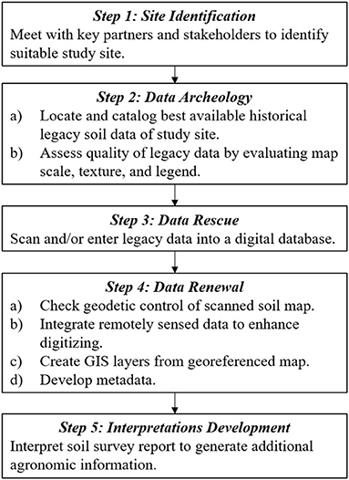
Figure 1. Conceptual flowchart showing the stepwise process for renewing archival legacy soil data.
Site Identification
Site identification, in our case, consisted of meetings with key institutions in Kenya, including the Academic Model Providing Access to Healthcare (AMPATH), Kenya Soil Survey, and the Kenya Agricultural and Livestock Research Organization (KALRO) to identify a setting for this study. Conversations with Dr. Joe Mamlin, AMPATH Field Director Emeritus, tasked us to identify a region in Kenya that has high population and poverty densities and high rates of people living with HIV/AIDS. These specifications are important for AMPATH because they want to have access to agronomic information and practices to test whether this will ultimately affect the quality of life of people living with HIV/AIDS from a nutritional standpoint. Discussions with the Kenya Soil Survey and KALRO were aimed at identifying a region in Kenya that meets the specifications described by AMPATH that also has detailed legacy soil data.
Data Archeology
The data archaeology step entails locating and cataloging legacy soil data available from key agricultural institutions. We retrieved legacy soil data from the Kenya Soil Survey in Nairobi. Kenya Soil Survey is the official government organization that stores all legacy soil data for the country.
Quality Assessment of Legacy Data
The guidelines described by Forbes et al. (15) were used to assess the quality of the legacy data by evaluating the map scale, texture, and legend. More specifically, this process is aimed at addressing: (i) whether the soil map is legible enough to represent the smallest land area of interest on paper maps to the user, (ii) whether the soil map conveys sufficient soil property information, (iii) whether control points and areas can be accurately located on the ground or map, and (iv) whether the map captures the soil development process for the target scale. In other words, for criterion iv, does the soil map use the catena concept to capture the soil variability within the landscape?
Map Scale and Texture
Map scale refers to “the relationship between the distances on the map and the corresponding distances on the ground,” whereas map texture refers to “the sizes and pattern of delineations on the map and determines the map's overall legibility” (15). Both the map scale and texture of the soil map were evaluated to assess the legibility and capability to represent the smallest area of interest. To do so, two map parameters were used. First was the minimum legible area (MLA) (Equation 1) that represents the smallest land area that can be represented on the map at its published scale using the criterion of a minimum legible delineation (MLD) of 0.4 cm2. The MLD is independent of the map scale and is conventionally defined to be a roughly circular area of 0.4 cm2. Smaller delineations are considered illegible for two reasons: (i) there is not enough room inside the delineation to legibly write the map unit symbol and (ii) the proportion of the delineation covered by the bounding line becomes significant. Second was the index of maximum reduction (IMR) (Equation 2), which refers to the factor by which the map scale can be reduced before the average size delineation (ASD) (Equation 3) would become equal to the MLD, i.e., before more than half of the map would become illegible. A large IMR implies that the survey area is represented on a map that is physically larger than necessary (15). The ASD is estimated using portions of a map with a given map texture by randomly sampling map areas with circles or squares of known areas and then converting the delineation counts in several of these areas (37). For this study, a transparent overlay with a 2.5 cm radius circle was used to count the number of delineations within the circle.
where the abbreviation RF stands for the representative fraction, which is the amount of any unit of distance measured on the ground that is represented by that unit on the map and is written as a ratio of two distances. For the Busia area, the RF is 1:100,000 meaning that 1 cm on the Busia soil map represents 100,000 cm (1000 m) on the ground.
The “sum of counts” refers to the number of delineations randomly selected within the transparent overlay.
Map Legend
The map legend identifies the map units based on the soil classification used (38). It refers to a full description in the associated survey report and may also provide a brief description and various interpretations. The legend can be identified by the symbols printed inside the map unit polygons. A descriptive legend gives information about each map unit, whereas the map unit names and definitions in descriptive and interpretative legends dictate the level of usefulness of the information. The map legend may be evaluated either in terms of a specific use of the soil inventory or by a more general criterion, such as a soil classification system (15). Map unit information was evaluated based on the availability of information on soil classification. Information is considered adequate if map unit descriptions included the diagnostic information such as horizons and properties, or the soil classification.
Data Rescue
Data rescue involves the transformation of the primary legacy data existing in paper format to an up-to-date archival format either by scanning or direct entry into a database (9, 39). Luckily, both the colored and the black-and-white soil maps of the study area were available in the European Soil Data Center (ESDAC) database http://esdac.jrc.ec.europa.eu/resource-type/national-soil-maps-eudasm (40). These maps had been scanned using a wide-format color scanner and were stored at 200 dpi (dots per inch) in TIFF (Tagged Image File Format), a lossless format that holds more detail than most other formats. Further processing of the digital maps such as cropping, distortion elimination, rotation, and color adjustment was carried out using an image-processing scanning software for wide-format images. Photo processing software was used to convert TIFF files into both JPEG and PDF formats (41). This process was replicated for the remaining Busia Area legacy soils data existing in paper format and not found in the ESDAC database (Table 1). The specifications of scanners, especially the color quality and resolution in terms of pixels per square are important considerations for preserving the authenticity of the original maps. In addition, all the available soil information contained within the scanned soil survey report [Appendices 3–6 in (42)] were manually entered into separate spreadsheet documents, saved as CSV (Comma Separated Values) text files, and stored for later use.
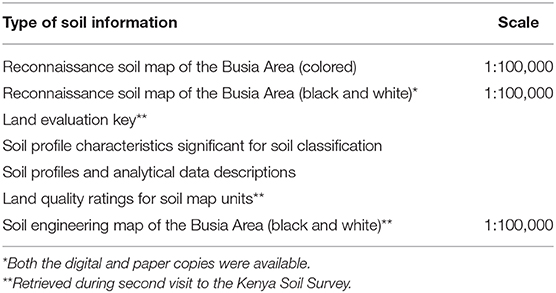
Table 1. Soil information contained within the Reconnaissance Soil Survey of the Busia Area.
Data Renewal
Data renewal involves the process of bringing legacy soil data to modern standards by taking advantage of technological and conceptual advances in geoinformation technology. These steps include georeferencing, digitalization, formatting for compatibility with GIS software, and metadata.
Geodetic Control
One drawback with most legacy soil maps is the lack of geodetic control points (4) for accurate georeferencing. This step involves looking for clearly labeled latitude and longitude points on the soil map to be used as the geodetic control points. Additional control points can also be identified using clues such as road intersections and rivers that are clearly visible on the available legacy soil map. These control points are used together with a suitable transformation available in ArcGIS (43) to shift and warp the scanned raster image from its existing location to the spatially correct location.
For georectification, satellite imagery was used as a basemap because it is freely available and provides the best currently available, up-to-date, georeferenced imagery of the study area. For this study, we used the satellite Imagery with Labels basemap from ArcGIS Online service. Key features on the soil map such as road intersections and natural features such as rivers were clearly visible on the scanned map and were used as additional control points for georectification. Forty control points evenly spread out across the study area were used for georectification and a third-order polynomial transformation was used to shift and warp the scanned map to its spatially correct location (RMSE = 6.63 × 10⁻⁴ m).
Integration of Remotely Sensed Data
Digitizing legacy soil maps often requires the integration of ancillary data, mostly remotely sensed data (9). Such products include Landsat imagery, vegetation cover, and terrain attributes that are generated from a digital elevation model (44). Soil is in part related to topography and vegetation (45, 46) and therefore the borders of some soil map units may align with remotely sensed data (13).
Creation of GIS Layers
This step involves the conversion of the georeferenced scanned soil paper map to a GIS layer by digitization. In cases where a digital copy of the soil map exists, this process can be omitted. One should, however, take caution with such digital copies and manually check if all the soil map units have been digitized and the soil map unit boundaries of the digital copy correctly overlay on the scanned soil map unit boundaries.
Development of Metadata
This step involves the development of appropriate metadata to include key identification information such as spatial data source, spatial reference, attributes, information on data quality, and description(s) of methods used to renew the data. The metadata also should include the explanation of key semantics used.
Interpretation of Soil Survey Information
This final step involves interpreting the soil classification information within the soil survey report to show and rate the best uses of the soil resources. This is because legacy data such as soil survey reports can provide basic information on soil and land characteristics that can be useful for various purposes such as determining the suitability for various types of practices for agricultural, range, and forestry land use.
For the Busia Area, the “Framework for Land Evaluation” prepared by FAO (47), was followed to develop additional agronomic information. Fundamental in this approach is that land can be classified meaningfully for clearly defined uses termed land use alternative types or land utilization types considered relevant for the survey area. Each land use type was defined by specific, quantifiable factors that have a marked influence on performance that is integral for defining crop suitability maps.
The Kenya Soil Survey prepared proposals for rating land qualities for the Busia Area [internal communication Nos. 7 and 29 (48, 49)]. In this rating system, land qualities were classified into three to five grades ranging from very low to very high based on the most limiting factor for the land qualities. The next step involved the establishment of specifications for the land qualities that will define the suitability class levels for each land use alternative. These steps were followed to generate land quality and crop suitability maps of the Busia Area. The suitability evaluation of each soil map unit for each land use alternative was carried out by comparing the land quality ratings of each soil map unit to the specifications for each land use alternative.
Results and Discussions
Site Identification
Meetings with AMPATH, KALRO, and the Kenya Soil Survey resulted in choosing the Busia Area as the setting for this study (Figure 2). This is because: (1) it has accessible detailed legacy soil data at a scale of 1:100,000 (42); (2) agriculture is the main economic activity in the area (50); (3) it has high population and poverty densities, and therefore provision of agronomic information is needed to revitalize agriculture in the area (51); (4) it has high rates of HIV/AIDS infections (52); and (5) the main author is from the study area and is familiar with it (13, 14). The site identification phase included numerous site visits with local partners who are familiar with the study area.
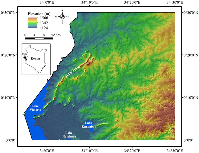
Figure 2. Geographic location of the Busia area.
Data Archeology
Available legacy soil data for the Busia Area, whether paper or digital formats, were manually retrieved by going through all field soil survey reports within the Kenya Soil Survey library (Figure 3). This effort resulted in the retrieval of the Reconnaissance Soil Survey of the Busia Area (quarter degree sheet No. 101) as the primary legacy soil data for this study (42). Table 1 shows the information contained within the soil survey report. This step requires care because information contained within the legacy soil data packet can easily be missed. After studying the soil survey report, maps, and tables obtained during our first visit, we identified missing materials, which required a second visit to the Kenya Soil Survey to obtain the missing information (Table 1). The best way to ensure that all the information is retrieved during the initial visit is by going through the table of contents of the soil survey report and paying attention to the appendix to ensure that all information is included the soil survey report packet. A reconnaissance visit to the study area was also conducted to familiarize ourselves with the area.
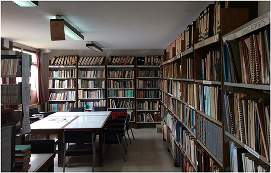
Figure 3. The Kenya Soil Survey library, June 6, 2017. Photo by Joshua O. Minai.
Quality Assessment of Legacy Data
Map Scale and Texture
The minimum legible area for the soil map of the Busia Area was 40 hectares (ha), which represents the smallest land area that can be represented on the map. The maximum location accuracy was 25 m, meaning that the inherent uncertainty on the ground of well-defined map points was 25 m. This directly affects the accuracy with which points on the ground may be represented. For a map scale to be adequate, the maximum location accuracy must be numerically smaller than the accuracy to which the user wishes to locate points on the ground and therefore depends upon the intended uses of the survey. A well-defined ground point can be plotted on the map sheet with an accuracy of 0.25 mm (53). The index of maximum reduction was 3.2, indicating that the map is very legible, and the map scale could be substantially reduced without impairing legibility.
Map Legend
Soil map units were explicitly labeled and categorized in the map legend (Table 2). The construction of the map unit legend indicated physiographic land types (such as hills, footslopes, uplands, etc.) based on physiographic photointerpretation. These land types were further subdivided according to the underlying parent material on which the soils were developed, described as either the stratigraphy or underlying rocks such as dolerites, granites, etc. At the third level the map units were broken down and described based on important soil profile characteristics including drainage conditions, depth, color, consistency, texture, etc. (42). This was then followed between brackets (dominant soils column in Table 2), by the classification of the main soils described according to the FAO/UNESCO nomenclature in the legend of the Soil Map of the World (38).
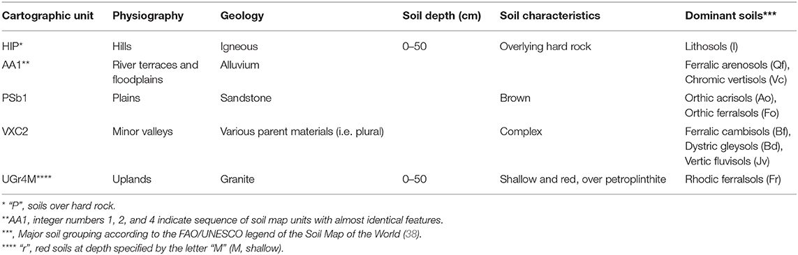
Table 2. Samples of soil map legend tables of the Busia Area, at 1:100,000 scale.
All the map units were explicitly described and therefore map units were adequately defined because the information within the map units provides sufficient specific information relative to the land use so that the map unit's suitability for a specific use may be determined and are uniform in their suitability for the land use i.e., 85% of their total area will perform similarly for the use. Map units contained descriptions of acreage, agro-ecological zone, parent material, meso- and macrorelief, erosion, vegetation, land use, general soil description, color, texture, structure, consistence, chemical properties, clay mineralogy, diagnostic properties, and soil classification according to the Soil Map of the World (38, 42).
Data Rescue
Most of the data in the soil survey report existed in paper formats. The survey report consists of the published report of the soil resources of the Busia Area itself, three map sheets, and two large folio sheets. The three map sheets included two soil maps of the Busia Area, one in color (Figure 4) and another in black-and-white [Appendices 1 and 2 in (42)], and a black-and-white soil engineering map [Appendix 7 in (42)]. The two large folio sheets included a land evaluation key [Appendix 3 in (42)] and soil profile characteristics significant for soil classification [Appendix 4 in (42)] (Table 1).
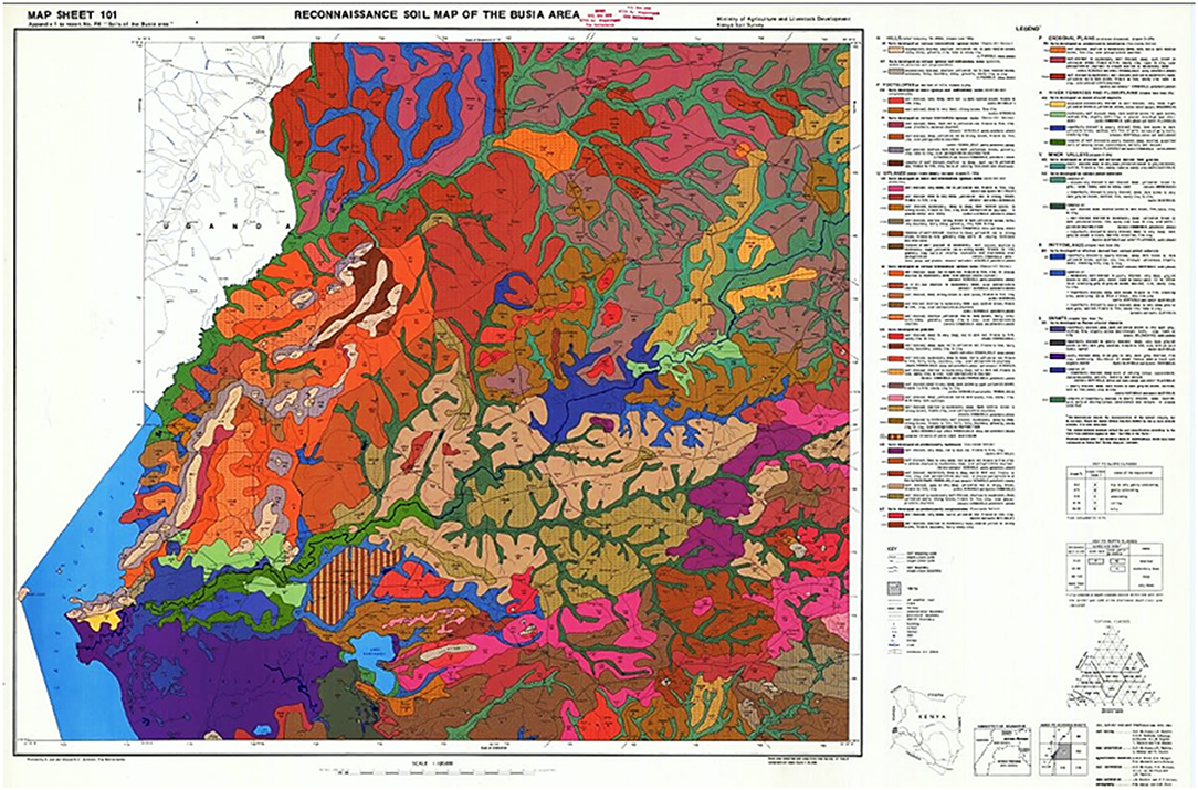
Figure 4. Rescued soil map of the Busia area at a scale of 1:100,000 from Panagos et al. (40) used with permission.
Data Renewal
Geodetic Control
The geodetic control points were available and legible, and both the geographic and grid coordinates were printed on the margins of the maps (Figure 5). The map projection was not given explicitly, but conversations with the Kenya Soil Survey GIS expert confirmed that the Busia Area soil map was developed using the East Africa War System of Coordinates, Traverse Mercator projection, belt I on the Arc 1960 datum with Clarke (54) as the reference ellipsoid (54). The map was first projected to Arc 1960 and then georeferenced using the four geodetic control points printed at the four corners of the map. It was then projected to the WGS84 Web Mercator (Auxiliary Sphere) projection.
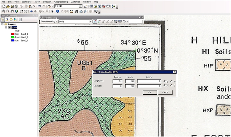
Figure 5. Geo-referencing of the reconnaissance soil map of the Busia area map using the top right corner geodetic control point. This geodetic control point is designated 34° 30′E, 0° 30′N.
GIS Coverages
The digitized soil map, provided by the Kenya Soil Survey, showed that the soil map units often were inaccurately delineated and did not capture key features such as islands and hills (Figure 6). This is a common challenge with paper maps because the transfer of the lines from field sheets to basemaps was not performed by surveyors. Without the soil surveyor's expert eye, knowledge, and experience, soil boundaries that followed obvious landscape features may have not been reproduced correctly, as described for other cases by Rossiter (9). This is expected because basemaps used by soil mappers available in the early 1980s were not as accurate compared to what is available today.
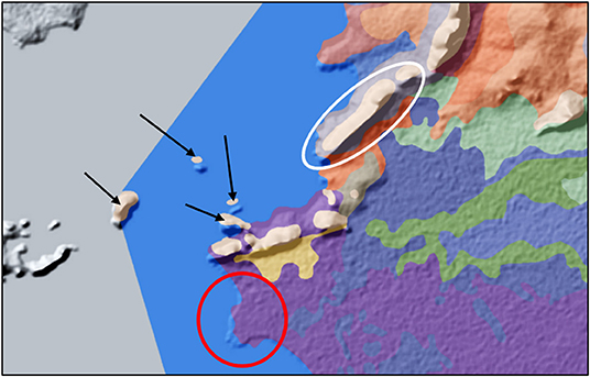
Figure 6. Using a hillshade to identify and correct inaccurately drawn soil map units. Black arrows show inaccurately drawn soil map units occurring on islands. Soil map unit within the red circle shows an incorrect boundary between that soil map unit and the water body. The soil map unit within the white boundary shows a map unit that is meant to represent soils of the hills.
Integration of Remotely Sensed Data
Rossiter (9) proposed the use of both satellite imagery and terrain attributes to adjust soil map unit boundaries. To ensure that each soil map unit captured its respective landscape features, satellite imagery and the hillshade generated from NASA's 30 m Shuttle Radar Topographic Mission (SRTM) (55) were used to manually adjust the polygon boundaries for some soil map units. Satellite imagery proved useful in correcting the soil map units that occurred on river terraces and swamps and for correcting boundaries between soil and water bodies, whereas the hillshade was used to adjust soil map unit boundaries on islands and hills (Figure 6). The integration of remotely sensed data resulted in a slight increase in the acreage of the soil map from 2,868 to 2,883 km2 (Table 3). This change is not considered significant and is likely to be due to either the projection of the digitized map into the Web Mercator (Auxilliary Sphere) projection, and/or to the fact that the surveyors probably determined soil map unit areas manually using a planimeter.
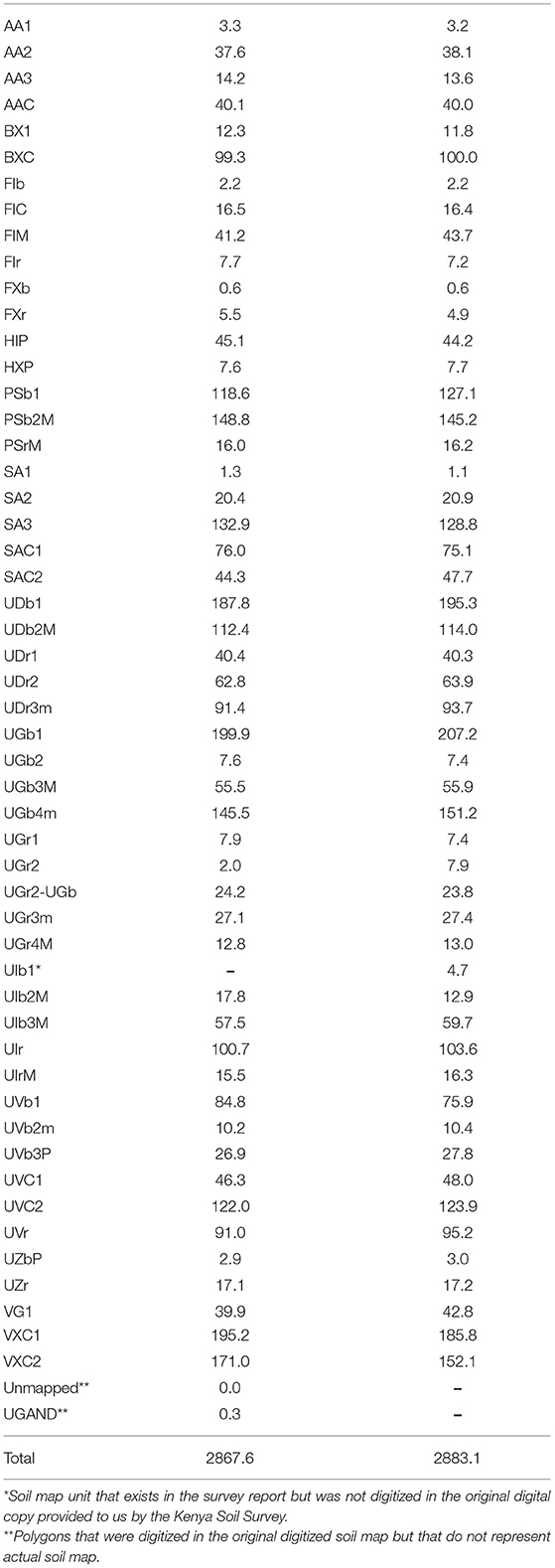
Table 3. Differences in soil map unit acreage between the original and the edited digitized soil map of the Busia Area.
Creation of GIS Layers
The result of the process described above was an accurately georeferenced, digitized soil map of the Busia Area with 348 polygons belonging to 52 different soil map units (Figure 7) broadly grouped into twelve soil orders (Table 4). Soil orders were determined from the taxonomic names of the soil classes in the soil map units. Most of the soils are moderately deep to deep, yellowish red to reddish brown, non-calcareous and predominantly kaolinitic in clay composition with few weatherable minerals remaining, and with evidence of a weak argillic horizon (42).
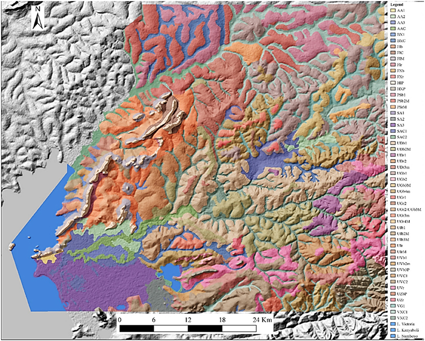
Figure 7. Digitized soil map of the Busia area. Colors of the soil map units are like those used by Rachilo and Michieka (42) and were determined and used to reproduce the map, which was then overlaid on the hillshade basemap with transparency set to 45% for a 3-dimensional effect.
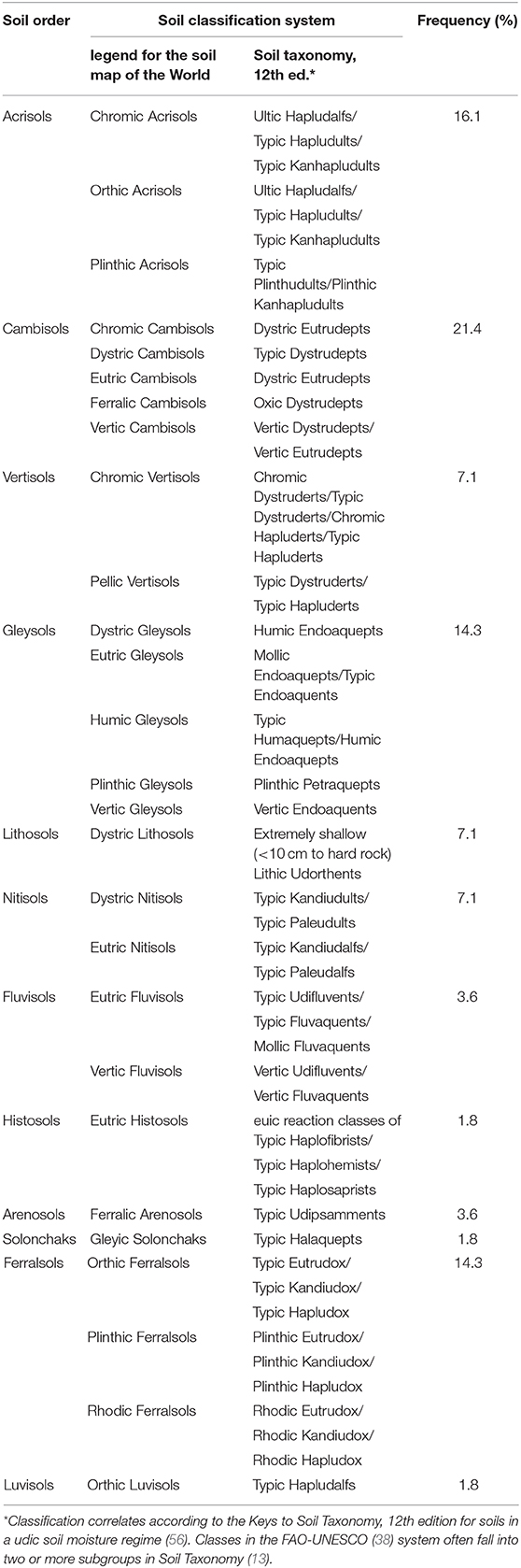
Table 4. Soil orders and soil classes of the Busia area according to the Legend for the Soil Map of the World (38) and correlates to the Soil Taxonomy, 12th edition (13).
Development of Metadata
Metadata included spatial data source, spatial reference, and processing steps (Table 5). Such documentation is useful because it allows other users to access the data, evaluate its usefulness for their intended purposes, and assist others in similar efforts to renew legacy soil data.
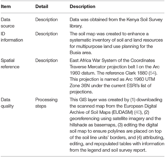
Table 5. Metadata information in the GIS layer of the Reconnaissance Soil Map of the Busia Area.
Soil Property Data
Two soil property datasets were also mined from the survey report. The first dataset consisted of 76 georeferenced locations for which A and B horizons were sampled [Appendix 4 in (42, 57)]. The A horizons were collected between depths of 0–30 cm for fertility analysis, whereas the B horizons were sampled to an unspecified depth. The soil properties included: texture, Munsell color, structure, consistence, the presence or absence of clay cutans, clay type, bulk density, porosity, soil classification according to both the FAO-UNESCO Soil Map of the World (38) and Soil Taxonomy (58), soil organic carbon (SOC), base saturation (at pH 7 and 8.2), exchangeable sodium percentage at pH 8.2 (ESP), and electrical conductivity (42). Of all these soil properties, data for SOC for the A horizon, texture for the A and B horizons, B/A clay ratio, and soil classification were available for all 76 profile pit locations (14).
The second set of soil property data consisted of detailed descriptions and analytical data for 48 georeferenced profile pits [pages 158 to 256 in (42, 57)]. Up to 15 soil properties were provided at different soil horizon depths. Latitudes and longitudes (in West Africa War System of Coordinates, Transverse Mercator projection, belt I on the Arc 1960 datum) for this dataset are contained within the soil profile descriptions [see page 159 in (42) as an example]. For more details see Hinga et al. (59).
Development of Interpretations
Land Quality Maps
Interpretation of the Busia Area soil survey report showed that land quality maps could be generated depending on the agro-ecological zone within which a specific soil type occurs. To show how these land qualities were generated using the information within the soil survey report, we demonstrate how the available soil moisture for plant growth was generated through the interpretation of the data. Even though in many publications the availability of moisture is defined as a soil property, the Busia Area soil survey report defines it as a land quality. However, the interpretation of the available soil moisture for plant growth needs to be related to the agro-ecological zones and the distribution of which may have been affected by climate change since the original soil survey was conducted. While available soil moisture capacity (AWC) is relatively stable the available soil moisture is dynamic and changes during the season depending on the interactions between crop type and climate.
Availability of Moisture for Crop Growth
This land quality expresses the period that a plant has adequate available soil water to support normal productive growth. The adequate available soil water is measured in terms of the presence of humid months without limitations for plant growth. The length of the accumulated growing months determines the suitability for a specific plant or crop (42).
Three different rooting depths, 0–50, 0–80, and 0–120 cm, were used to determine the total available soil moisture capacity for the crop growing months. This approach was explicitly described in the legacy soil survey report [pages 127 and 128 in (42)]. Since soil moisture also is climate-dependent, the agro-climatic map of Kenya was used to map out the different agro-climatic zones in the Busia Area. Four different agro-climatic zones (I, II, III, and IV) were mapped (60). For example, agro-climatic zone I has 11 growing months available for 0–50 and 0–80 cm soil depth and 11.5 months for 0–120 cm soil depth. For agro-ecological zones II to IV, see Tables 11–13 in Rachilo and Michieka (42).
The length of growing season(s) in months was further grouped according to the land quality rating (Table 6). The length of the growing season in this example represents available soil moisture under the assumption that a longer growing season translates to more available soil moisture during the growing season. We computed the land quality ratings for each soil map unit [Appendix 6 in (42)] and used this to map out the availability of soil moisture for the study area (Figure 8). The map of available soil moisture is consistent with what we would expect on this landscape. Hills have low available moisture because the soils are very shallow, consisting of Lithosols with stony phases. Conversely, river terraces and swamps have soils with high available moisture since these are depositional areas where water accumulates.
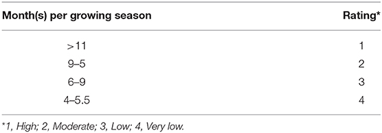
Table 6. Ratings for the availability of moisture for plant growth [Table 14 in (42)].
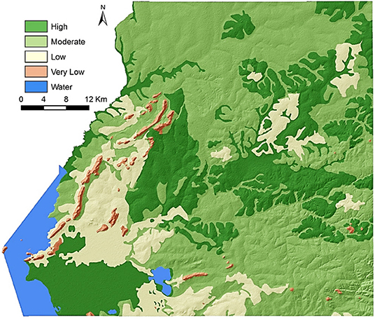
Figure 8. Availability of moisture for plant growth for the Busia Area.
Similar stepwise approaches were used to map nine additional land quality categories for the study area including: (i) temperature, (ii) availability of nutrients for plant growth, (iii) salinity hazard, (iv) sodicity hazard, (v) erosion susceptibility, (vi) availability of oxygen in the root zone, (vii) flooding hazards, (viii) seedbed preparation and cultivation potential, and (ix) availability of foothold for roots. See Appendix A in Minai (61) and Minai and Schulze (62) to view and download these land quality maps. Although the renewed maps are more consistent from the soil-landscape relationship perspective, their utility is still limited due to lack of field validation.
Crop Suitability Maps
The ratings for the 10 land qualities developed by Rachilo and Michieka (42) were further used to determine suitability classes for specific crops [Tables 32–49 in (42)]. All the land qualities were applied to individual soil mapping units (plural) to determine their suitability for specific crops. We utilized this information in the form of decision matrices to delineate suitability classes for agronomic crops suitable for the study area.
Suitability Class Map for Rainfed Maize
Table 7 [also Table 40 in (42)] was used as the decision matrix to determine the suitability for each soil map unit to support rainfed maize (Zea mays L.) growing under intermediate technology. Using this decision matrix, we generated if-then (conditional) statements to determine the suitability of each soil map unit in the Busia Area for rainfed maize. The Join and Relate tools in ArcMap were used to combine the newly created suitability class table with the Busia Area soil map attribute table to delineate the suitability for rainfed maize under intermediate technology for the study area (Figure 9).
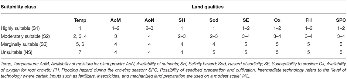
Table 7. Decision matrix for the suitability classification of soils for rainfed maize growing under the intermediate technology option [Table 40 in (42)].
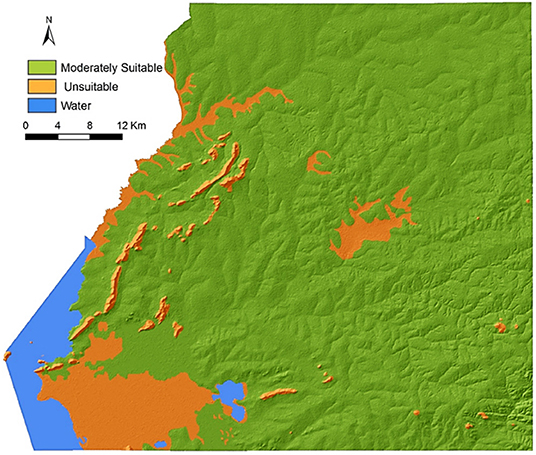
Figure 9. Maize (Zea mays L.) crop suitability map for the Busia area.
Rachilo and Michieka (42) developed a detailed land evaluation key and decision matrix, showing land suitability classifications for various activities and land use types for all the soil map units within the study area across all four agro-ecological zones [Appendix 3 in (42)]. This decision matrix was used, following similar approaches for developing the suitability map for maize, to produce suitability class maps for additional 18 crops, including (1) sugarcane (Saccharum officinarum L.), (2) cabbages (Brassica oleracea var. capitata L.), (3) kale (Brassica oleracea var. viridis L.), (4) onions (Allium cepa L.), (5) tomatoes (Lycopersicon esculentum L.), (6) wetland and upland rice (Oryza glaberrima Steud.), (7) citrus guava (Psidium guajava L. ), (8) cotton (Gossypium hirsutum L.), (9) groundnuts (Arachis hypogaea L.), (10) maize (Zea mays L.), (11) finger millet (Eleusine coracana L.), (12) cassava (Manihot esculenta Crantz), (13) common beans (Phaseolus vulgaris L.), (14) sunflower (Helianthus annuus L.), (15) Robusta coffee [Coffea canephora var. robusta (L. Linden) A. Chev)], (16) forestry, (17) fodder crops, and (18) areas suitable for grazing. See Appendix B in (61), and (63) to view and download the crop suitability maps, respectively.
These maps offer the first attempt to generate additional land quality and crop suitability maps generated from interpretation of an existing soil survey report. These products, however, may need substantial improvement because they are based on agronomic data collected over 40 years ago. Since then, several of the underlying factors used to determine the suitability classes for these crops have likely changed significantly (64). Additional field studies are needed to generate new land quality maps for the study area. For example, current climatic conditions such as temperature and rainfall amount and distribution may not reflect past climatic conditions (65). Similarly, chemical soil property data used to determine land quality ratings for the study area are not static (66). Many soil properties such as organic matter, available phosphorus, exchangeable K, Ca, and Mg, pH-H2O, can vary even within a growing season (67).
Digital Soil Mapping
The availability of georeferenced soil property from the survey report allowed us to map soil organic carbon and texture using digital soil mapping techniques (14, 61). Similarly, a soil landscape rule-based approach was used to disaggregate the traditional soil polygon map of the survey area into individual soil classes at a spatial resolution of 30 m (13).
Conclusion
This study aimed at renewing the best available soil survey report of a selected portion of Kenya into a digital format and using the information in the legacy data to support the provision of additional agronomic information. The Reconnaissance Soil Survey of the Busia Area (quarter degree sheet No. 101) was used as an example. Interpretation of the agronomic information in the legacy report resulted in the development of 10 land quality maps and 18 different crop suitability maps that were previously not available.
We demonstrated the feasibility of delivering some of these maps via the cellphone network in rural Kenya. The Exploratory Soil Map of Kenya (1982), the Reconnaissance Soil Map of the Busia Area, and three additional maps of the Busia area were published to a server and then made available in the Soil Explorer mobile app for iOS and Android devices and in the SoilExplorer.net website. We were able to access these maps in the field on an Apple iPad Mini connected to the Safaricom cellphone network (61, 68).
The process of legacy data rescue first resulted in georeferenced soil property data. These data allowed us to map selected soil properties (soil organic carbon and texture for the surface horizon) using digital soil mapping techniques (14). The same information was also used to disaggregate the traditional soil map into individual soil classes within soil map units at a spatial resolution of 30 m using a soil landscape rule-based approach (13). These map products currently are the best available high-resolution soil maps for soil organic carbon and texture for the Busia Area and exemplify the ability to map soil properties using digital soil mapping techniques solely based on data from a previously published soil survey report.
We hope that the procedures described above will provide a blueprint for the rescue of legacy soil data for other areas. Additionally, digital soil mapping can benefit from renewed legacy data as the legacy soil data can provide inputs into digital soil mapping projects.
Data Availability Statement
The raw data supporting the conclusions of this article are available without reservation as per citations in the article.
Author Contributions
JM, DS, and ZL contributed to the conception of the study. JM conducted reconnaissance visits, legacy data archeology, and write-up of the manuscript with contributions of DS and ZL. All authors read and approved the submitted manuscript.
Funding
This work was made possible by funding from the Purdue Center for Global Food Security and the Purdue University Libraries Open Access Publishing Fund. ZL was supported in part by LE STUDIUM Loire Valley Institute for Advanced Studies through its LE STUDIUM Research Consortium Programme.
Conflict of Interest
The authors declare that the research was conducted in the absence of any commercial or financial relationships that could be construed as a potential conflict of interest.
Publisher's Note
All claims expressed in this article are solely those of the authors and do not necessarily represent those of their affiliated organizations, or those of the publisher, the editors and the reviewers. Any product that may be evaluated in this article, or claim that may be made by its manufacturer, is not guaranteed or endorsed by the publisher.
Acknowledgments
We would like to acknowledge the assistance given to us by the Kenya Soil Survey department staff who made available the necessary legacy data for this study. We thank Mr. Geoffrey Macharia, Head, Kenya Soil Survey and Mr. Lucas Tanui, GIS specialist, Kenya Soil Survey, for providing existing legacy soil data for this study. Sincere thanks go to the Kenya Agricultural and Livestock Research Organization (KALRO) and the Academic Model Providing Access to Healthcare staff (AMPATH) for their assistance in identifying the study location. The authors would like to express their gratitude to Jenny Sutherland at the United States Department of Agriculture, National Soil Survey Center, Soil and Plant Science Division for her extensive and numerous editing and reviews of the manuscript.
References
1. Zinck JA, . (Ed.). Soil Survey: Perspectives and Strategies for the 21st Century (No. 21). Rome: Food and Agriculture Org. (1995).
2. McBratney AB, Santos MM, Minasny B. On digital soil mapping. Geoderma. (2003) 117:3–52. doi: 10.1016/S0016-7061(03)00223-4
3. Odeh IO, Leenaars J, Hartemink A, Amapu I. The challenges of collating legacy data for digital mapping of Nigerian soils. In: Budiman M, Brendan M, Alex MB, editors. Digital Soil Assessments and Beyond. London: Taylor and Francis (2012). doi: 10.1201/b12728-88
4. Cambule AH, Rossiter DG, Stoorvogel JJ, Smaling EMA. Rescue and renewal of legacy soil resource inventories: a case study of the Limpopo national park, Mozambique. Catena. (2015) 125:169–82. doi: 10.1016/j.catena.2014.10.019
5. Cook SE, Jarvis A. A new global demand for digital soil information. In: Digital Soil Mapping with Limited Data. Springer Verlag. The Netherlands (2008). p. 31–41. doi: 10.1007/978-1-4020-8592-5_3
6. Arrouays D, Leenaars J. G., Richer-de-Forges AC, Adhikari K, Ballabio C, Greve M, et al. Soil legacy data rescue via GlobalSoilMap and other international and national initiatives. Geo Res J. (2017) 14:1–19. doi: 10.1016/j.grj.2017.06.001
7. Kenya Soil Survey. List of Publications of the Kenya Soil Survey From 1972 Onwards. Nairobi: Ministry of Agriculture (1986). p. 37.
9. Rossiter DG. Digital soil mapping as a component of data renewal for areas with sparse soil data infrastructures. In: Digital Soil Mapping with Limited Data. Dordrecht: Springer the Netherlands (2008). p. 69–80. doi: 10.1007/978-1-4020-8592-5_6
10. Baxter SJ, Crawford DM. Incorporating legacy soil pH databases into digital soil maps. In: Digital Soil Mapping with Limited Data. Dordrecht: Springer (2008). p. 311–8. doi: 10.1007/978-1-4020-8592-5_27
11. Krol B. G. C. M. Towards a data quality management framework for digital soil mapping with limited data. In: Digital Soil Mapping with Limited Data. Dordrecht: Springer (2008). p. 137–49. doi: 10.1007/978-1-4020-8592-5_11
12. Rasaei Z, Rossiter DG, Farshad A. Rescue and renewal of legacy soil resource inventories in Iran as an input to digital soil mapping. Geoderma Reg. (2020) 21:e00262. doi: 10.1016/j.geodrs.2020.e00262
13. Minai J, Libohova Z, Schulze DG. Disaggregation of the 1: 100,000 reconnaissance soil map of the Busia Area, Kenya using a soil landscape rule-based approach. Catena. (2020) 195:104806. doi: 10.1016/j.catena.2020.104806
14. Minai JO, Libohova Z, Schulze DG. Spatial prediction of soil properties for the Busia area, Kenya using legacy soil data. Geoderma Reg. (2021) 25:e00366. doi: 10.1016/j.geodrs.2021.e00366
15. Forbes TR, Rossiter D, Van Wambeke A. Guidelines for Evaluating the Adequacy of Soil Resource Inventories. 1987 Printing ed. Ithaca, NY: Cornell University Department of Agronomy (1982).
16. Goodchild MF, Hunter GJ. A simple positional accuracy measure for linear features. Int J Geogr Inform Sci. (1997) 11:299–306. doi: 10.1080/136588197242419
17. Dent DL, Ahmed FB. Resurrection of soil surveys: a case study of the acid sulphate soils of The Gambia. I Data validation, taxonomic and mapping units. Soil Use Manag. (1995) 11:69–76. doi: 10.1111/j.1475-2743.1995.tb00499.x
18. Ahmed FB, Dent DL. Resurrection of soil surveys: a case study of the acid sulphate soils of The Gambia. II Added value from spatial statistics. Soil Use Manag. (1997) 13:57–9. doi: 10.1111/j.1475-2743.1997.tb00557.x
19. Hengl T, Toomanian N, Reuter HI, Malakouti MJ. Methods to interpolate soil categorical variables from profile observations: lessons from Iran. Geoderma. (2007) 140:417–27. doi: 10.1016/j.geoderma.2007.04.022
20. Ugbaje SU, Reuter HI. Functional digital soil mapping for the prediction of available water capacity in Nigeria using legacy data. Vadose Zone J. (2013) 12:1–13. doi: 10.2136/vzj2013.07.0140
21. Hengl T, de Jesus JM, MacMillan RA, Batjes NH, Heuvelink GB, Ribeiro E, et al. SoilGrids1km—global soil information based on automated mapping. PLoS ONE. (2014) 9:e105992. doi: 10.1371/journal.pone.0105992
22. Skinner RJ, Todd AD. Twenty-five years of monitoring pH and nutrient status of soils in England and Wales. Soil Use Manag. (1998) 14:162–9. doi: 10.1111/j.1475-2743.1998.tb00144.x
23. Cahoon LB, Ensign SH. Spatial and temporal variability in excessive soil phosphorus levels in eastern North Carolina. Nutrient Cycl. Agroecosyst. (2004) 69:111–25. doi: 10.1023/B:FRES.0000029676.21237.54
24. Wheeler DM, Sparling GP, Roberts AHC. Trends in some soil test data over a 14-year period in New Zealand. New Zeal J Agric Res. (2004) 47:155–66. doi: 10.1080/00288233.2004.9513583
25. Baxter SJ, Oliver MA, Archer JR. The spatial distribution and variation of available Phosphorus in agricultural topsoil in England and Wales in 1971, 1981, 1991 and 2001. Dev Soil Sci. (2006) 31:477–626. doi: 10.1016/S0166-2481(06)31035-5
26. Lemercier B, Gaudin L, Walter C, Aurousseau P, Arrouays D, Schvartz C, et al. Soil phosphorus monitoring at the regional level by means of a soil test database. Soil Use Manag. (2008) 24:131–8. doi: 10.1111/j.1475-2743.2008.00146.x
27. Saby NPA, Arrouays D, Antoni V, Lemercier B, Follain S, Walter C, et al. Changes in soil organic carbon in a mountainous French region, 1990–2004. Soil Use Manag. (2008) 24:254–62. doi: 10.1111/j.1475-2743.2008.00159.x
28. Reijneveld JA, Ehlert PAI, Termorshuizen AJ, Oenema O. Changes in the soil phosphorus status of agricultural land in the Netherlands during the 20th century. Soil Use Manag. (2010) 26:399–411. doi: 10.1111/j.1475-2743.2010.00290.x
29. Stockmann U, Padarian J, McBratney A, Minasny B, de Brogniez D, Montanarella L, et al. Global soil organic carbon assessment. Glob Food Security. (2015) 6:9–16. doi: 10.1016/j.gfs.2015.07.001
30. Sleutel S, De Neve S, Hofman G. Assessing causes of recent organic carbon losses from cropland soils by means of regional-scaled input balances for the case of Flanders (Belgium). Nutrient Cycl Agroecosyst. (2007) 78:265–78. doi: 10.1007/s10705-007-9090-x
31. Goidts E, Van Wesemael B, Crucifix M. Magnitude and sources of uncertainties in soil organic carbon (SOC) stock assessments at various scales. Eur J Soil Sci. (2009) 60:723–39. doi: 10.1111/j.1365-2389.2009.01157.x
32. Meersmans J, van Wesemael B, Goidts E, Van Molle M, De Baets S, De Ridder F. Spatial analysis of soil organic carbon evolution in Belgian croplands and grasslands, 1960–2006. Glob Chang Biol. (2011) 17:466–79. doi: 10.1111/j.1365-2486.2010.02183.x
33. Dobos E, Bialkó T, Micheli E, Kobza J. Legacy soil data harmonization and database development. In: Digital Soil Mapping. Dordrecht: Springer (2010). p. 309–23. doi: 10.1007/978-90-481-8863-5_25
34. Leenaars JGB. Africa Soil Profiles Database, Version 1.0: A Compilation of Georeferenced Standardised Legacy Soil Profile Data for Sub-Saharan Africa (with dataset). Wageningen, the Netherlands: Africa Soil Information Service (AfSIS) project ISRIC — World Soil Information (2012). p. 45. Available online at: http://www.isric.org. ISRIC report 2012/03 (accessed January 11, 2019).
35. Leenaars JGB. Africa Soil Profiles Database, Version 1.1. A Compilation of Georeferenced and Standardised Legacy Soil Profile Data for Sub-Saharan Africa (with dataset). Africa Soil Information Service (AfSIS) project (No. 2013/03). ISRIC-World Soil Information (2013).
36. Leenaars JG, Van Oostrum AJM, Ruiperez Gonzalez M. Africa Soil Profiles Database Version 1.2. A Compilation of Georeferenced and Standardized Legacy Soil Profile Data for Sub-Saharan Africa (with dataset). Wageningen: ISRIC Report 2014/01; 2014. ISRIC-World Soil Information, Wageningen (2014).
37. Laker MC. “Selection of a Method for Determination of Map intensities of Soil Maps,” in Soil Resource Inventories and Development Planning: Selected Papers from the Proceedings of Workshops New York: Soil Management Support Services, Soil Conservation Services, US Department of Agriculture. (1979). p. 339.
39. Hoffman KM, Clarke CT, Shiue HSY, Nicholas P, Shaw M, Fenlon K. Data Rescue: An Assessment Framework for Legacy Research Collections. College Park: University of Maryland College of Information Studies. (2020).
40. Panagos P, Jones A, Bosco C, Kumar PS. European digital archive on soil maps (EuDASM): preserving important soil data for public free access. Int J Digit Earth. (2011) 4:434–43. doi: 10.1080/17538947.2011.596580
42. Rachilo JR, Michieka DO. Reconnaissance Soil Survey of the Busia Area (Quarter Degree Sheet No. 101). Nairobi: Kenya Soil Survey (1991).
44. Conrad O, Bechtel B, Bock M, Dietrich H, Fischer E, Gerlitz L, et al. System for Automated Geoscientific Analyses (SAGA) v. 2.1.4. Geosci Model Dev. (2015) 8:1991–2007. doi: 10.5194/gmd-8-1991-2015
45. Jenny H. Soil genesis with ecological perspectives. Ecol Stud. (1980). 37:276–360. doi: 10.1007/978-1-4612-6112-4
46. Jenny H. Factors of Soil Formation: A System of Quantitative Pedology. New York: Courier Corporation (1994).
48. Braun HMH, Van de Weg RF. Proposals for Rating of Land Qualities. Internal Communications, (7). Nairobi: Kenya Soil Survey (1977).
49. Fertilizer Use Recommendation Project (FURP). Description of first priority trial sites in the various districts, Ministry of Agriculture/NAL/FURP, Final Report-Annex III: Vol. 4, Siaya district to Vol. 31, Kwale district. Nairobi, Kenya: National Agricultural Laboratories (1988).
50. Onywere SM, Getenga ZM, Mwakalila SS, Twesigye CK, Nakiranda JK. Assessing the challenge of settlement in Budalangi and Yala swamp area in Western Kenya using landsat satellite imagery. Open Environ Eng J. (2011) 4:97–104. doi: 10.2174/1874829501104010097
51. Kenya National Bureau of Statistics. Kenya National Bureau of Statistics (KNBS) Kenya 2009 Population and Housing Census Highlights. Nairobi: KNBS Government of Kenya. (2010).
53. Davis RE, Foote FS, Anderson JM, Mikhail EM. Surveying, Theory and Practice. 6th ed. New York, NY: McGraw-Hill (1981). p. 992.
55. USGS. Digital Elevation Model Dataset. (2017). Available online at: : https://earthexplorer.usgs.gov/ (accessed April 11, 2017).
56. Soil Survey Staff. Keys to Soil taxonomy. 12th ed. Washington, DC: USDA-Natural Resource Conservation Service (2014).
57. Minai JO, Schulze DG. Soil Property Data for Spatial Prediction of Soil Properties for the Busia Area, Kenya. West Lafayette, IN: Purdue University Research Repository (2019).
58. Soil Survey Staff. Soil Taxonomy, a Basic System of Soil Classification for Making and Interpreting Soil Surveys. United States Department of Agriculture, Handbook No. 436. Washington, DC: U.S. Government Printing Office (1975).
59. Hinga G, Muchena FN, Njihia CM. Physical and Chemical Methods of Soil Analysis. Nairobi: National Agricultural Research Laboratories (1980).
60. Sombroek WG, Braun HMH, Van der Pouw BJA. Exploratory Soil Map and Agro-Climatic Zone Map of Kenya, 1980. Scale 1: 1,000,000. Nairobi: Kenya Soil Survey (1982).
61. Minai JO. Utilization of legacy soil data for digital soil mapping and data delivery for the Busia Area, Kenya (Doctoral dissertation). West Lafayette, IN: Purdue University Graduate School (2019).
62. Minai JO, Schulze DG. Data from: Busia Land Quality Maps. Purdue University Research Repository (2019).
63. Minai JO, Schulze DG. Data from: Busia Crop Suitability Maps. West Lafayette, IN: Purdue University Research Repository (2019).
64. Tittonell PABLO, Vanlauwe B, de Ridder N, Giller KE. Heterogeneity of crop productivity and resource use efficiency within smallholder Kenyan farms: soil fertility gradients or management intensity gradients? Agric Syst. (2007) 94:376–90. doi: 10.1016/j.agsy.2006.10.012
65. Fick SE, Hijmans RJ. WorldClim 2: new 1-km spatial resolution climate surfaces for global land areas. Int J Climatol. (2017) 37:4302–15. doi: 10.1002/joc.5086
66. Moebius-Clune BN, Van Es HM, Idowu OJ, Schindelbeck RR, Kimetu JM, Ngoze S, et al. Long-term soil quality degradation along a cultivation chronosequence in western Kenya. Agric Ecosyst Environ. (2011) 141:86–99. doi: 10.1016/j.agee.2011.02.018
67. Nyberg G, Bargués Tobella A, Kinyangi J, Ilstedt U. Soil property changes over a 120-yr chronosequence from forest to agriculture in western Kenya. Hydrol Earth SystSci. (2012) 16:2085–94. doi: 10.5194/hess-16-2085-2012
68. Minai JO, Ngunjiri MW, Schulze DG, Owens PR, Serrem C, Nyabinda N. (2016). Delivery of Spatially Explicit Soils Information in Western Kenya. Abstract Retrieved from Abstracts in Soil Science Society of America International Annual Meeting, November 6-9, 2016, Phoenix, Arizona. Available online at: https://scisoc.confex.com/scisoc/2016am/webprogram/Paper100855.html (accessed Jan 12, 2020).
Keywords: Busia, data archeology, data rescue, data renewal, land quality map, crop suitability map
Citation: Minai JO, Schulze DG and Libohova Z (2022) Renewal of Archival Legacy Soil Data: A Case Study of the Busia Area, Kenya. Front. Soil Sci. 1:765248. doi: 10.3389/fsoil.2021.765248
Received: 26 August 2021; Accepted: 15 December 2021;
Published: 26 January 2022.
Edited by:
Vera Leatitia Mulder, Wageningen University and Research, NetherlandsReviewed by:
Dominique Arrouays, Institut National de la Recherche Agronomique (INRA), FranceLuboš Boru˙vka, Czech University of Life Sciences Prague, Czechia
Brendan Malone, Commonwealth Scientific and Industrial Research Organisation (CSIRO), Australia
Copyright © 2022 Minai, Schulze and Libohova. This is an open-access article distributed under the terms of the Creative Commons Attribution License (CC BY). The use, distribution or reproduction in other forums is permitted, provided the original author(s) and the copyright owner(s) are credited and that the original publication in this journal is cited, in accordance with accepted academic practice. No use, distribution or reproduction is permitted which does not comply with these terms.
*Correspondence: Joshua O. Minai, am1pbmFpQHB1cmR1ZS5lZHU=