Equilibrium configurations in a nematic pi-cell under an electric field

In this work, we study the equilibrium configurations in a nematic pi-cell under an electric field using the one-dimensional Oseen-Frank director model. The equilibrium orientational configurations that can be attained in a pi-cell are known as splay, bend, and twist. Among those, bend and twist are topologically equivalent and can be transitioned into one another as voltage varies. The transition can be continuous or abrupt depending on the material parameters. On the other hand, the splay configuration becomes asymmetric for sufficiently high voltages if the liquid crystal has a positive dielectric anisotropy. We determine those threshold voltages and characterize the order of transitions in terms of the elastic constants and the pretilt angle at the boundary.

1 Introduction

A multistable-state device has two or more locally stable states which are separated by energy barriers. The transitions among the states can be realized by applying an external field large enough to overcome the energy barrier to reach another state. After the field is removed, the device will remain in its locally stable state without a constant supply of power. Some known bistable devices include cholesteric liquid crystal (LC) display (Yang et al., 1994), bistable twist nematic (BTN) (Berreman and Heffner, 1980), surface controlled bistable nematic (Berreman and Heffner, 1981; Dozov and Durand, 1998; Kim et al., 2001), and Zenithally bistable nematic device (Bryan-Brown et al., 1994), just to name a few.

In 1980, Boyd, Cheng, and Ngo (Boyd et al., 1980) proposed a nematic LC display, later referred to as the pi-cell: nematic liquid crystals are enclosed between two parallel substrates; the boundaries are conditioned to induce the same pretilt alignment, characterized by the polar angle θ₀ of the directors at the plate surfaces; and the top plate is rotated by angle π relative to the bottom plate, see Figure 1A. Three locally stable configurations, known as horizontal (H) for predominately splay, vertical (V) for predominately bend, and twist (T) states, can be achieved by specifying appropriate boundary conditions and proper material parameters. Switching among the topologically distinct states (V/T and H) can be realized via formation and movement of disclinations near the bounding surfaces after the application of electric and magnetic fields.

FIGURE 1

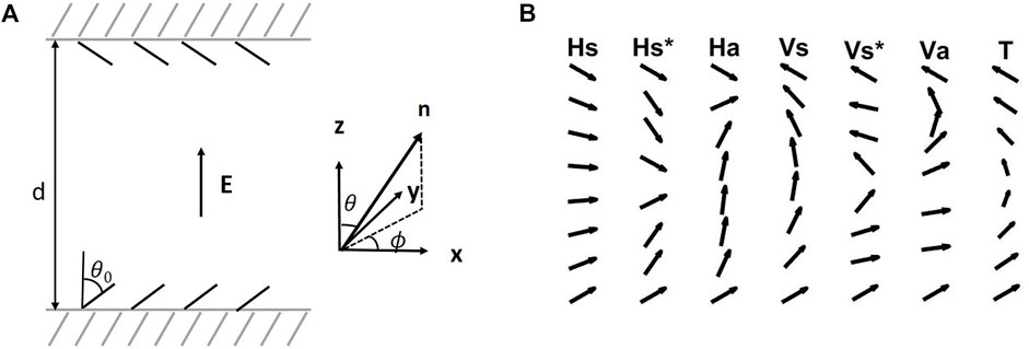
FIGURE 1. (A) A schematic of the nematic pi-cell with boundary pretilt conditions θ₀, showing the coordinate system and definitions of angles θ and ϕ for the director n. (B) A schematic showing seven possible equilibrium orientation patterns of a nematic pi-cell under a vertical electric field. They are referred to as monotonic symmetric splay (Hs), nonmonotonic symmetric splay (Hs*), asymmetric splay (Ha), monotonic symmetric bend (Vs), nonmonotonic symmetric bend (Vs*), asymmetric bend (Va), and twist (T). The director field is assumed to be uniform in a plane parallel to the bounding plates.

In 1984 (Bos and Koehler/Beran, 1984), demonstrated that the pi-cell can be used for fast optical-switching devices in the V-state, also known as optically compensated bend (OCB) mode. Since then, many liquid crystal display devices with fast response time, large viewing angles, and high transmittance have been proposed based on the pi-cell (Yu and Kwok, 2004; Jhun et al., 2006; Wu et al., 2012; Lin et al., 2015; Zhou et al., 2017).

There are seven possible equilibrium orientational patterns of a nematic pi-cell under an electric field applied normal to the cell, as shown in Figure 1; three are predominately splay configurations, which we label as Hs, Hs*, and Ha, three are predominately bend configurations, which we label as Vs, Vs*, and Va, and one is the out-of-plane twist configuration, which we label as T. Here Hs stands for monotonic symmetric splay where the tilt angle θ(z) monotonically increases from the bottom plate to the midplane, Hs* is for nonmonotonic symmetric splay where the tilt angle θ(z) first decreases and then increases from bottom plate to the midplane, and Ha represents the asymmetric splay. Similarly, Vs is for monotonic symmetric bend where the tilt angle θ(z) monotonically decreases from bottom plate to the midplane, Vs* is for nonmonotonic symmetric bend where the tilt angle θ(z) first increases and then decreases from bottom to the midplane, and Va for the asymmetric bend. Among them, the Hs* and Ha configurations can only be found for LCs with positive dielectric anisotropy under sufficiently strong field. Similarly, Vs* and Va exist only for LCs with negative dielectric anisotropy under sufficiently strong field but, as we shall show, are unstable to twist state (T). The director field in the plane parallel to the bounding plates is assumed to be uniform.

In this work, we aim at a thorough parameter study of equilibrium configurations in a nematic pi-cell under an electric field. We do not consider the switching among the topologically distinct configurations in this work. The paper is organized as follows. Section 2 introduces the mathematical model, where the distortion energy of the director field in the pi-cell is modeled with the one-dimensional Oseen-Frank elastic theory, and the electric field satisfies the Maxwell equations. The Euler-Lagrange equations and the corresponding first integrals for the equilibrium configurations are derived. In Section 3, the results of the equilibrium configurations in the absence of electric field are presented in terms of the elastic constants and the boundary pretilt angle. In Section 4, we show the effect of the electric field on the equilibrium configurations. We summarize the paper in Section 5.

2 Mathematical model

In this section, we first present the free energy of the system, featuring the Oseen-Frank elastic energy and the electric energy. We then derive the Euler-Lagrange equations and corresponding first integrals which determine the equilibrium director fields.

2.1 Free energy

In this work, we assume that the orientation field of the nematic liquid crystal is uniaxial and has a constant scalar order parameter throughout the cell, thus can be described by the unit vector field n(x). We take the free energy due to the distortion in the director field n as given by Oseen-Frank theory (Oseen, 1933; Frank, 1958),

$\begin{array}{ll}\hfill F_{OF}& =\frac{1}{2}{\int }_{\mathrm{\Omega }}{K}_1{\left(\nabla \cdot \mathbf{n}\right)}^2+K_2{\left(\mathbf{n}\cdot \nabla \times \mathbf{n}\right)}^2+K_3|\mathbf{n}\times \nabla \times \mathbf{n}{|}^2\hfill \\ \hfill & +\left(K_2+K_4\right)\nabla \cdot \left[\left(\mathbf{n}\cdot \nabla \right)\mathbf{n}-\left(\nabla \cdot \mathbf{n}\right)\mathbf{n}\right]dV.\hfill \end{array}(1)$

Here K₁, K₂, and K₃ are the elastic constants corresponding to splay, twist, and bend distortions, respectively, and the combination K₂ + K₄ is the saddle-splay constant. This energy is bounded from below if K₁ ≥ 0, K₂ ≥ 0, K₃ ≥ 0, K₂ ≥|K₄|, and 2K₁ ≥ K₂ + K₄ ≥ 0 (Ericksen, 1966). The last term, known as null Lagrangian, can be integrated by divergence theorem and becomes a surface term, which depends on the director variation along the bounding surface. Since we consider strong anchoring on the surface, this becomes an additive constant in the energy, thus can be ignored.

The electric energy is given by (cf. (Lagerwall, 1999))

$F_E=-\frac{1}{2}{\int }_{\mathrm{\Omega }}\mathbf{D}\cdot \mathbf{E}dV,(2)$

where the electric displacement is D = ɛ(n)E, with the dielectric tensor

$\epsilon ={\epsilon }_0\left({\epsilon }_{\perp }\mathbf{I}+\left({\epsilon }_{\Vert }-{\epsilon }_{\perp }\right)\mathbf{n}\mathbf{n}\right).(3)$

The constants ɛ_‖ and ɛ_⊥ are the relative dielectric permittivities of the liquid crystal when the field is parallel and perpendicular to the director, respectively. The difference ɛ_a = ɛ_‖ − ɛ_⊥ is the dielectric anisotropy of the liquid crystal. For materials with positive dielectric anisotropy, that is, ɛ_a > 0, the molecules prefer to align parallel with the electric field; whereas for materials with negative dielectric anisotropy, that is, ɛ_a < 0, the molecules prefer to align perpendicular to the electric field.

It is well known that the electric field will be altered by the director distortion, whereas the influence of the director on the magnetic field is negligible (Deuling, 1972; Gartland, 2020). An accurate model of electric field involves solving the Maxwell’s equations

$\nabla \cdot \mathbf{D}=0,\nabla \times \mathbf{E}=0,(4)$

under the assumption that there are no free charges in the cell. The curl free condition on the electric field gives immediately E = −∇U, where U is the electric potential. In this work, we consider that the electric potential difference is applied parallel to the normal of the bounding plates along the z − direction, and assume that both the director field and electric field are functions of z, that is

$\mathbf{E}\left(z\right)=-\frac{dU}{dz}\left(\mathrm{0,0,1}\right),(5)$

and the director n(z) adopts the usual parametrization

$\mathbf{n}\left(z\right)=\left(\sin \theta \left(z\right)\cos \varphi \left(z\right),\sin \theta \left(z\right)\sin \varphi \left(z\right),\cos \theta \left(z\right)\right),(6)$

where the polar angle θ is measured from z − axis, and the azimuthal angle ϕ is measured from x − axis. Following the similar treatment as in (Deuling, 1972), the z − component of electric displacement D(z) is a constant, that is,

$D\left(z\right)=D={\epsilon }_0\left({\epsilon }_{\perp }+{\epsilon }_a{\cos }^2\theta \right)E,(7)$

and the electric potential difference across the cell is

$U_0=-{\int }_0^{d}E\left(z\right)dz=-D{\epsilon }_0^{-1}{\int }_0^d{\left({\epsilon }_{\perp }+{\epsilon }_a{\cos }^2\theta \right)}^{-1}dz.(8)$

We note that there is no singularity in the integrand since ɛ_a/ɛ_⊥ > −1. With Eq. 8, the electric energy (2) can be written as

$F_E=-\frac{A}{2}{U}_0^2{\epsilon }_0{\left({\int }_0^d{\left({\epsilon }_{\perp }+{\epsilon }_a{\cos }^2\theta \right)}^{-1}dz\right)}^{-1},(9)$

where A is the area of the bounding plates, and d is the gap thickness.

We define the following dimensionless parameters,

$k_1=\frac{K_1-K_3}{K_3},k_2=\frac{K_2-K_3}{K_3},\bar{z}=\frac{\pi z}{d},\alpha =\frac{{\epsilon }_0{\epsilon }_a{U}_0^2}{K_3{\pi }^2},\bar{U}=\frac{U}{\sqrt{K_3{\pi }^2/|{\epsilon }_0{\epsilon }_a|}},\gamma ={\epsilon }_a{\epsilon }_{\perp }^{-1},(10)$

where k₁, k₂, γ ∈ (−1, ∞), the cell thickness is rescaled to π, and the parameter α, which is proportional to $U_0^2$, has the same sign as that of ɛ_a and γ. Then the total bulk free energy, which is the sum of the Oseen-Frank elastic energy and the electric energy, can be expressed as,

$F_{\mathit{tot}}=\frac{K_{3}A\pi }{2d}\left({\int }_0^{\pi }f\left(\theta \right){\theta }^{\prime 2}+g\left(\theta \right){\varphi }^{\prime 2}d\bar{z}-\alpha {\pi }^2{\left({\int }_0^{\pi }{\left({\gamma }^{-1}+{\cos }^2\theta \right)}^{-1}d\bar{z}\right)}^{-1}\right),(11)$

where ${()}^{\prime }=d()/d\bar{z}$ and

$f\left(\theta \right)=1+k_1{\sin }^2\theta ,(12)$

$g\left(\theta \right)=\left(1+k_2{\sin }^2\theta \right){\sin }^2\theta .(13)$

The electric field, $\bar{E}(\bar{z})=-{\bar{U}}^{\prime }$, can be solved from

${\left(\left({\gamma }^{-1}+{\cos }^2\theta \right){\bar{U}}^{\prime }\right)}^{\prime }=0,(14)$

$\bar{U}\left(0\right)=0,\bar{U}\left(\pi \right)=\sqrt{|\alpha |}.(15)$

It is also useful to define the dimensionless parameter $\delta =\frac{D^2{d}^2}{{\epsilon }_0{\epsilon }_a{K}_3{\pi }^2}$. With it, Eq. 7 becomes

$\delta =\mathrm{sign}\left({\epsilon }_a\right){\pi }^2{\left({\gamma }^{-1}+{\cos }^2\theta \right)}^2{\bar{U}}^{\prime 2},(16)$

and α and δ are related, via Eq. 8, as

$\alpha {\pi }^2=\delta {\left({\int }_0^{\pi }{\left({\gamma }^{-1}+{\cos }^2\theta \right)}^{-1}d\bar{z}\right)}^2.(17)$

Using Eq. 17, the total free energy in (11) can be written as

$F_{\mathit{tot}}=\frac{K_{3}A\pi }{2d}\left({\int }_0^{\pi }f\left(\theta \right){\theta }^{\prime 2}+g\left(\theta \right){\varphi }^{\prime 2}d\bar{z}-\delta {\int }_0^{\pi }{\left({\gamma }^{-1}+{\cos }^2\theta \right)}^{-1}d\bar{z}\right).(18)$

We will use this equation for subsequent calculations for the energies of the equilibrium configurations. For convenience, we drop the bar from the variable $\bar{z}$, such that in the subsequent sections, z is the nondimensionalized spatial variable ranging from 0 to π.

2.2 Euler-Lagrange equations and first integrals

Setting the first variations of the free energy functional in Eq. 11 with respect to θ and ϕ to zeros, and utilizing Eq. 17, we obtain the Euler-Lagrange (EL) equations for θ and ϕ,

$2{\theta }^{\prime \prime }f\left(\theta \right)+{\theta }^{\prime 2}{f}^{\prime }\left(\theta \right)-{\varphi }^{\prime 2}{g}^{\prime }\left(\theta \right)-\delta \frac{\sin 2\theta }{{\left({\gamma }^{-1}+{\cos }^2\theta \right)}^2}=0,(19)$

${\varphi }^{\prime \prime }g\left(\theta \right)+{\theta }^{\prime }{\varphi }^{\prime }{g}^{\prime }\left(\theta \right)=0.(20)$

Eqs 19, 20, with δ replaced with Eq. 16, together with Eqs 14, 15 and boundary conditions for θ and ϕ, are readily solved by any numerical solver for ODE boundary value problems.

Multiplying Eq. 19 by θ′, Eq. 20 by ϕ′, adding them together, and integrating the result with respect to z, we obtain a first integral

$f\left(\theta \right){\theta }^{\prime 2}+g\left(\theta \right){\varphi }^{\prime 2}-\frac{\delta }{{\gamma }^{-1}+{\cos }^2\theta }=C.(21)$

Integrating Eq. 20 with respect to z yields another first integral

$g\left(\theta \right){\varphi }^{\prime }=k.(22)$

Here C and k are constants of integration. We note that from Eqs 18, 21, the free energy density is invariant in space and is proportional to the integration constant C.

Since the director fields of splay and bend configurations are constrained to lie in a plane orthogonal to the bounding plates, ϕ(z) is a constant, and the EL equations reduce to a single equation for θ(z). The boundary conditions for splay, bend, and twist configurations differ drastically because of the different underlying topologies. To conveniently describe the transitions among different configurations, we further manipulate those differential equations, together with symmetry properties and boundary conditions, to obtain algebraic equations which, upon solving, give the essential quantities associated with each configuration, e.g. integration constants C and k, the extreme tilt angle θ_m, and energy F. We discuss the details for each configuration separately in the subsections below.

2.2.1 Splay configuration

For the splay configuration, the azimuthal angle ϕ(z) is constant, so Eq. 22 is automatically satisfied with k = 0, and Eq. 21 simplifies to

$f\left(\theta \right){\theta }^{\prime 2}-\frac{\delta }{{\gamma }^{-1}+{\cos }^2\theta }=C_S.(23)$

Separating the variables, we get

$dz=\pm \sqrt{\frac{f\left(\theta \right)}{C_S+\frac{\delta }{{\gamma }^{-1}+{\cos }^2\theta }}}d\theta ,(24)$

where the plus sign is adopted if θ increases with z, and the minus sign is adopted otherwise. Eq. 24 provides the implicit relation between θ and z.

The boundary conditions specifying the pretilt angles for the splay configuration are given by

$\theta \left(0\right)={\theta }_0,(25)$

$\theta \left(\pi \right)=\pi -{\theta }_0,(26)$

where 0 ≤ θ₀ ≤ π/2, and are illustrated in Figure 1B, where the pretilt angles are formed by the director n at the boundary plates with the positive z − axis for the Hs, Hs*, and Ha configurations. Eqs 17, 24–26 determine the solution θ(z) for the splay configuration for given θ₀ and α.

Below, we comment briefly on the monotonicity of θ(z) and its associated symmetry property. We first show that in the absence of electric field, the solution θ(z) for the splay configuration is monotonic. If θ₀ = π/2, then θ(z) ≡ π/2, which is automatically monotonic. If θ₀ ≠ π/2, the monotonicity can be shown by contradiction. Since if otherwise, θ(z) possesses a local extremum at an interior point z = z∗ such that θ′(z∗) = 0, then θ′(z) ≡ 0 by setting δ = 0 in Eq. 23, and θ(z) is a constant, violating the boundary conditions Eqs. 25, 26. As we shall show in Section 4, monotonic splay configurations only exist if α is smaller than a positive threshold value α_cs, beyond which θ(z) becomes nonmonotonic.

Furthermore, if θ(z) is monotonic, the plus sign is taken in Eq. 24. Integrating Eq. 24 in (0, z), we have

$z={\int }_{{\theta }_0}^{\theta \left(z\right)}\sqrt{\frac{1+k_1{\sin }^2\theta }{C_S+\frac{\delta }{{\gamma }^{-1}+{\cos }^2\theta }}}d\theta \stackrel{\widehat{\theta }=\pi -\theta }{=}{\int }_{\pi -\theta \left(z\right)}^{\pi -{\theta }_0}\sqrt{\frac{1+k_1{\sin }^2\widehat{\theta }}{C_S+\frac{\delta }{{\gamma }^{-1}+{\cos }^2\widehat{\theta }}}}d\widehat{\theta },(27)$

and integrating Eq. 24 in (π − z, π) gives

$z={\int }_{\theta \left(\pi -z\right)}^{\pi -{\theta }_0}\sqrt{\frac{1+k_1{\sin }^2\theta }{C_S+\frac{\delta }{{\gamma }^{-1}+{\cos }^2\theta }}}d\theta .(28)$

Equating the right hand sides of Eqs 27, 28, we obtain the symmetry property for monotonic θ(z), that is,

$\theta \left(\pi -z\right)=\pi -\theta \left(z\right).(29)$

Further manipulations of equations are different for monotonic and nonmonotonic splay configurations, which we defer to Sections 3 and 4.

2.2.2 Bend configuration

The EL equation for bend configuration is the same as that for splay configuration,

$f\left(\theta \right){\theta }^{\prime 2}-\frac{\delta }{{\gamma }^{-1}+{\cos }^2\theta }=C_B.(30)$

So is the implicit relation between θ and z,

$dz=\pm \sqrt{\frac{f\left(\theta \right)}{C_B+\frac{\delta }{{\gamma }^{-1}+{\cos }^2\theta }}}d\theta .(31)$

The boundary conditions for bend configuration are

$\theta \left(0\right)={\theta }_0,(32)$

$\theta \left(\pi \right)=-{\theta }_0,(33)$

with 0 ≤ θ₀ ≤ π/2. Eqs 17, 31–33 determine the solution θ(z) for the bend configuration for given θ₀ and α.

Similar to the splay configuration, the solution θ(z) for bend configuration is monotonic in the absence of electric field and continues to be monotonic for α > α_cb, with the threshold value α_cb < 0. For α < α_cb, θ(z) becomes nonmonotonic. With the similar argument as in the splay configuration, one can show that if θ(z) is monotonic, it satisfies the symmetry property

$\theta \left(\pi -z\right)=-\theta \left(z\right).(34)$

2.2.3 Twist configuration

For twist configuration, one has to solve the full set of Eqs 17, 21, 22, together with boundary conditions

$\theta \left(0\right)={\theta }_0,\varphi \left(0\right)={\varphi }_0,(35)$

$\theta \left(\pi \right)={\theta }_0,\varphi \left(\pi \right)={\varphi }_0\pm \pi ,(36)$

where 0 ≤ θ₀ ≤ π/2, and ϕ₀ is an arbitrary angle. We set ϕ₀ = 0 such that the director on the boundary lies in the xz − plane. The boundary condition ϕ(π) = ϕ₀ + π is for the right-handed twist configuration, and ϕ(π) = ϕ₀ − π is for left-handed twist: each is equally probable. We focus on the right-handed twist for further analysis.

We seek the solution θ(z) in twist configuration which is unimodal, that is, θ(z) possesses only one local extreme for z ∈ (0, π). Generally speaking, if θ(z) possesses multiple local extremum points, the corresponding configuration often has high energy due to the rapid variations in θ(z), so we do not consider those solutions. Following the similar line of argument as for the splay configuration, we can show that if θ(z) is a unimodal function, then θ(z) is symmetric with respect to the midplane, that is

$\theta \left(\pi /2\right)={\theta }_m,{\theta }^{\prime }\left(\pi /2\right)=0,\theta \left(z\right)=\theta \left(\pi -z\right),0\le z\le \frac{\pi }{2}.(37)$

Meanwhile, one can also establish the symmetric relation for ϕ(z), using Eq. 22,

$\varphi \left(\pi -z\right)=\pi -\varphi \left(z\right),0\le z\le \frac{\pi }{2}.(38)$

Combining Eqs 21, 22, 37, we get

$C_T=-\frac{\delta }{{\gamma }^{-1}+{\cos }^2{\theta }_m}+\frac{k^2}{g\left({\theta }_m\right)}.(39)$

Separating the variables in Eq. 21, via Eqs 22, 39, yields

$dz=\pm \sqrt{\frac{f\left(\theta \right)}{\frac{\delta }{{\gamma }^{-1}+{\cos }^2\theta }-\frac{\delta }{{\gamma }^{-1}+{\cos }^2{\theta }_m}+k^2\left(\frac{1}{g\left({\theta }_m\right)}-\frac{1}{g\left(\theta \right)}\right)}}d\theta .(40)$

Integrating Eq. 40 from z = 0 to z = π/2 leads to

$\frac{\pi }{2}={\int }_0^{\pi /2}dz=\pm {\int }_{{\theta }_0}^{{\theta }_m}{\left[\frac{f\left(\theta \right)}{\frac{\delta }{{\gamma }^{-1}+{\cos }^2\theta }-\frac{\delta }{{\gamma }^{-1}+{\cos }^2{\theta }_m}+k^2\left(\frac{1}{g\left({\theta }_m\right)}-\frac{1}{g\left(\theta \right)}\right)}\right]}^{1/2}d\theta .(41)$

Similarly, by Eqs 22, 38, 40, we obtain

$\frac{\pi }{2}={\int }_0^{\pi /2}\frac{k}{g\left(\theta \right)}dz=\pm {\int }_{{\theta }_0}^{{\theta }_m}{\left[\frac{f\left(\theta \right)}{\frac{\delta }{{\gamma }^{-1}+{\cos }^2\theta }-\frac{\delta }{{\gamma }^{-1}+{\cos }^2{\theta }_m}+k^2\left(\frac{1}{g\left({\theta }_m\right)}-\frac{1}{g\left(\theta \right)}\right)}\right]}^{1/2}\frac{k}{g\left(\theta \right)}d\theta .(42)$

In Eqs 41, 42, the positive signs are taken for increasing θ(z) or θ_m > θ₀, which we refer to as a large tilt twist, and the negative signs are taken for decreasing θ(z) or θ_m < θ₀, which we refer to as a small tilt twist.

Eqs 41, 42 relate θ₀, θ_m, δ, and k. Given any two quantities, we can solve for the other two. It is important to point out that there might be zero, one, or two values of θ_m corresponding to a given θ₀, as shown in Figures 2–4 in Section 3. The direct method which solves θ_m in terms of α and θ₀ is an involved procedure, especially when the number of solutions is not known a priori (Scheffer, 1978). However, there is always a unique value θ₀ for each given θ_m ∈ [0, π/2]. With this, our strategy is to solve for θ₀ for a given θ_m. First, for a given set of δ/k² and θ_m, the pretilt angle at the boundary θ₀ is numerically solved from Eq. 42. In this work, we used the FindRoot function in Wolfram Mathematica 10 as our numerical solver. Knowing the values of θ₀, k can be evaluated by multiplying Eq. 41 by k throughout. Next, α can be obtained by Eq. 17, which can be written, upon substituting Eq. 40 and rearranging, as

$\alpha =\frac{4\delta }{{\pi }^2}{\left({\int }_{{\theta }_0}^{{\theta }_m}\frac{k}{{\gamma }^{-1}+{\cos }^2\theta }{\left[\frac{f\left(\theta \right)}{\frac{\delta /k^2}{{\gamma }^{-1}+{\cos }^2\theta }-\frac{\delta /k^2}{{\gamma }^{-1}+{\cos }^2{\theta }_m}+\left(\frac{1}{g\left({\theta }_m\right)}-\frac{1}{g\left(\theta \right)}\right)}\right]}^{1/2}d\theta \right)}^2.(43)$

FIGURE 2

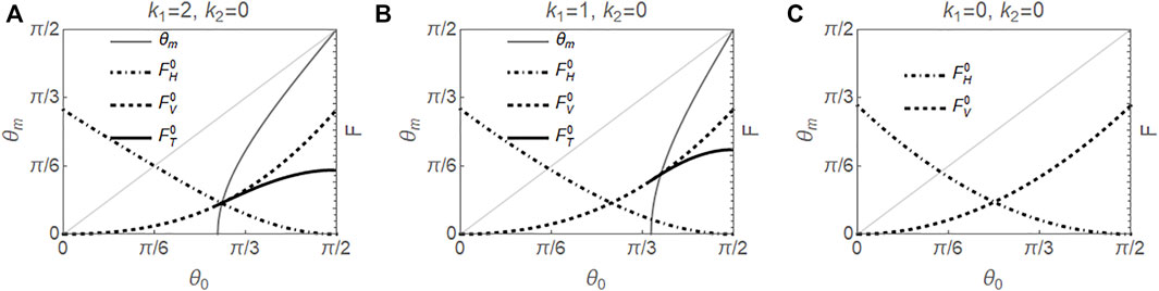
FIGURE 2. Results for k₂ = 0 in the absence of electric field. Left axes show θ_m vs. θ₀ for the twist configuration, and right axes show the scaled energies for splay $(F_H^0)$, bend $(F_V^0)$, and twist $(F_T^0)$ configurations vs. θ₀. For (A) k₁ = 2, there is a second order transition from bend to twist. For (B) k₁ = 1, there is a second order transition at a larger θ₀. For (C) k₁ = 0, there is no twist solution.

This enables us to relate the tilt angle θ_m at the midplane with θ₀ and α. Furthermore, the energy for the resulting configuration can be expressed as

$F_T=\frac{K_{3}A{\pi }^2}{2d}{C}_T=\frac{K_{3}A{\pi }^2}{2d}\left(\frac{1}{g\left({\theta }_m\right)}-\frac{\delta /k^2}{{\gamma }^{-1}+{\cos }^2{\theta }_m}\right)k^2.(44)$

Special cares have to be taken in the above procedure, since in both Eqs 41, 42, the radicand cannot be negative, and proper signs need to be chosen based on the monotonicity of θ(z). Since f(θ) > 0, the denominator of the radicand has to be positive, that is,

$h\left(\theta \right)=\frac{\delta /k^2}{{\gamma }^{-1}+{\cos }^2\theta }-\frac{\delta /k^2}{{\gamma }^{-1}+{\cos }^2{\theta }_m}+\left(\frac{1}{g\left({\theta }_m\right)}-\frac{1}{g\left(\theta \right)}\right)>0,(45)$

for θ in between θ₀ and θ_m. We note that since h(θ_m) = 0, the sign of h′(θ_m) alone determines the monotonicity of θ(z) such that the nonnegative requirement of the radicand is satisfied. Specifically, if h′(θ_m) > 0, then θ is necessarily greater than θ_m to ensure h(θ) > 0. This gives θ₀ > θ_m, hence θ′ < 0, and the minus signs are adopted in Eqs. 41, 42. If h′(θ_m) < 0, θ is necessarily less than θ_m to satisfy h(θ) > 0, thus θ₀ < θ_m, which gives θ′ > 0, and the positive signs are adopted. If h′(θ_m) = 0, then θ₀ = θ_m. In this special case, the twist configuration has a constant tilt angle and a uniform twist with ϕ′ = 1. From Eqs 22, 17, we obtain k = g(θ₀) and $\alpha =\delta /{({\gamma }^{-1}+{\cos }^2{\theta }_0)}^2$. Subsequently, the energy can be evaluated by Eq. 44.

It is important to note that in the limiting case of θ_m → 0, ϕ(z) approaches a step function with ϕ = 0 at the lower half and ϕ = π at the upper half of the cell, with ϕ not uniquely defined at the midplane. This is illustrated by the dotted curves in Figure 11 in Section 4. Due to the head-to-tail symmetry of n, that is, n and − n refer to the same orientation, we recognize that twist configuration becomes bend as θ_m → 0. Since twist configuration can be transformed to a bend configuration through a continuous mapping, and vice versa, those two configurations are topologically equivalent.

3 Solutions in the absence of electric field

Let’s first consider the equilibrium configurations in a pi-cell without the electric field. We first obtain the energies for splay, bend, and twist equilibrium configurations in Sections 3.1, 3.2 and 3.3, and the results are shown in Section 3.4.

3.1 Splay configuration

We showed earlier in Section 2.2.1 that in the absence of electric field, θ(z) for splay configuration is monotonic, hence satisfies the symmetry relation Eq. 29, which gives θ(π/2) = π/2. Setting δ = 0 in Eq. 23, we obtain C_S = (1 + k₁)θ′(π/2)². Since θ(z) is increasing, the plus sign is taken in Eq. 24. Integrating Eq. 24 from z = 0 to z = π/2 and rearranging gives

${\theta }^{\prime }\left(\pi /2\right)=\frac{2}{\pi }{\int }_{{\theta }_0}^{\pi /2}\sqrt{\frac{f\left(\theta \right)}{1+k_1}}d\theta .(46)$

Together with Eqs 18, 23, the energy for the splay configuration can be written as

$F_H^0=\frac{K_{3}A{\pi }^2}{2d}{C}_S=\frac{K_{3}A}{2d}{\left({\int }_{{\theta }_0}^{\pi -{\theta }_0}\sqrt{f\left(\theta \right)}d\theta \right)}^2.(47)$

It can be readily shown that the energy for the splay configuration increases with k₁ and decreases with θ₀.

3.2 Bend configuration

Similarly, for bend configuration, the symmetry relation Eq. 34 implies θ(π/2) = 0. Setting δ = 0 in Eq. 30, we have C_B = θ′(π/2)². Since θ(z) is monotonically decreasing, the negative sign is taken in Eq. 31. Integrating Eq. 31 from z = 0 to z = π/2 and rearranging gives

${\theta }^{\prime }\left(\pi /2\right)=\frac{2}{\pi }{\int }_{{\theta }_0}^0\sqrt{f\left(\theta \right)}d\theta .(48)$

The energy for the bend configuration, using Eqs 18, 30, can be written as

$F_V^0=\frac{K_{3}A{\pi }^2}{2d}{C}_B=\frac{K_{3}A}{2d}{\left({\int }_{{\theta }_0}^{-{\theta }_0}\sqrt{f\left(\theta \right)}d\theta \right)}^2.(49)$

It follows that the energy for the bend configuration increases with both k₁ and θ₀.

3.3 Twist configuration

If δ = 0, Eq. 45 simplifies to

$h\left(\theta \right)=\frac{1}{g\left({\theta }_m\right)}-\frac{1}{g\left(\theta \right)},(50)$

and the sign of h′(θ_m) follows that of g′(θ_m). Given θ_m, θ₀ is solved from Eq. 42, which by setting δ = 0, becomes

$\frac{\pi }{2}=\pm \sqrt{g\left({\theta }_m\right)}{\int }_{{\theta }_0}^{{\theta }_m}{\left[\frac{f\left(\theta \right)}{g\left(\theta \right)\left(g\left(\theta \right)-g\left({\theta }_m\right)\right)}\right]}^{1/2}d\theta ,(51)$

where the plus sign is taken if g′(θ_m) < 0, and the minus sign is taken otherwise. Once θ₀ and θ_m are known, k can be evaluated by setting δ = 0 in Eq. 41 and rearranging, that is,

$k=\frac{2}{\pi }{\int }_{{\theta }_0}^{{\theta }_m}{\left[\frac{f\left(\theta \right)g\left(\theta \right)g\left({\theta }_m\right)}{g\left(\theta \right)-g\left({\theta }_m\right)}\right]}^{1/2}d\theta .(52)$

Together with Eqs 21, 22, one obtains C_T = k²/g(θ_m), and the corresponding energy for the twist configuration can be evaluated as

$F_T^0=\frac{K_{3}A{\pi }^2}{2d}{C}_T=\frac{K_{3}A}{2d}{\left(2{\int }_{{\theta }_0}^{{\theta }_m}{\left[\frac{f\left(\theta \right)g\left(\theta \right)}{g\left(\theta \right)-g\left({\theta }_m\right)}\right]}^{1/2}d\theta \right)}^2.(53)$

3.4 Results

In this section, we show the results of equilibrium configurations in a pi-cell in the absence of electric field with three representative values of k₂ = 0, −0.5, −0.75, and k₁ is allowed to vary continuously from −1 to ∞.

3.4.1 k₂ = 0

For k₂ = 0, since g′(θ_m) = sin 2θ_m > 0 for θ_m ∈ (0, π/2), the minus sign was adopted when solving Eq. 51, and θ_m < θ₀. Therefore all twist solutions, if they exist, have small tilt angles in the midplane, as shown in Figure 2 where the solid curves for θ_m lie below the diagonal. Figure 2 also shows energies of equilibrium splay, bend, and twist solutions as functions of θ₀, calculated from Eqs 47, 49, 53, respectively.

For higher values of k₁, as θ₀ increases, there is a twist solution branching from the bend solution as a supercritical bifurcation, indicating a second order transition, as shown in Figures 2A,B. Beyond the bifurcation point, the twist solution corresponds to a local minimum energy state, and bend solution corresponds to a saddle point in the energy landscape. The bifurcation point moves towards π/2 as k₁ decreases and becomes larger than π/2 and nonphysical at k₁ = 0, as shown in Figure 2C, where there is no twist solution for any θ₀ ∈ (0, π/2). We note that the case of k₁ = k₂ = 0 corresponds to the situation usually referred to as the one constant approximation.

On the other hand, the splay solution always corresponds to a local minimum energy state. The energy curves of splay and bend intersect at a θ_0c, which increases with k₁. In particular, the two energies are the same when θ_0c = π/6 for k₁ → −1, θ_0c = π/4 if k₁ = 0, and θ_0c = π/3 as k₁ → ∞.

3.4.2 k₂ = −0.5

The parameter k₂ = −0.5 is a typical value for MBBA (Haller, 1972; Leger, 1972). Similar to the case of k₂ = 0, since $\mathrm{g\prime }$(θm) = cos²θ_m sin 2θ_m > 0 for θ_m ∈ (0, π/2), all twist solutions for k₂ = −0.5 have a small tilt angle in the midplane with θ_m < θ₀. The main difference from the results of k₂ = 0 is that the supercritical bifurcation from bend to twist for larger values of k₁, as shown in Figure 3A, becomes subcritical as k₁ decreases, as shown in Figures 3B,C, signifying a first order transition. In Figure 3C, the bifurcation point is larger than π/2, and the part of the curve for θ₀ > π/2 was cut off from the plot since it is not physical.

FIGURE 3

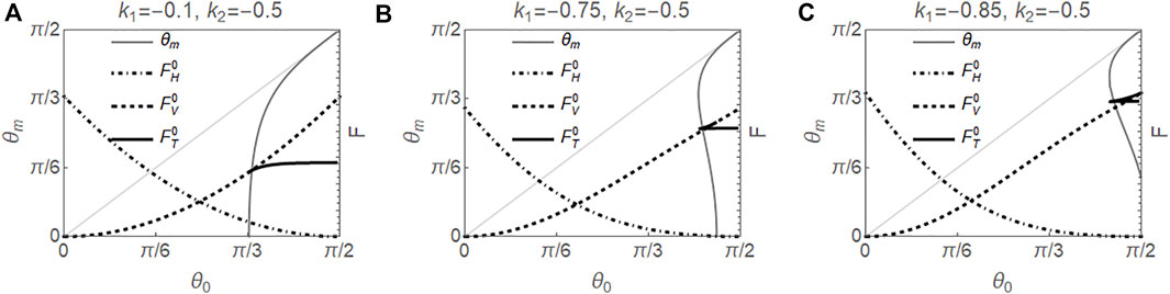
FIGURE 3. Results for k₂ = −0.5 in the absence of electric field. Left axes show solutions θ_m vs. θ₀ for the twist configuration, and right axes show the scaled energies for splay $(F_H^0)$, bend $(F_V^0)$, and twist $(F_T^0)$ configurations vs. θ₀. For (A) k₁ = −0.1, there is a second order transition from bend to twist. For (B) k = −0.75, there is a first order transition from bend to twist. For (C) k₁ = −0.85, there is a first order transition from bend to twist, but the bifurcation point for θ_m moves out of physical range. We note that the first order transition occurs when the bend and twist energy curves intersect.

In the case that there are two twist configurations for a given θ₀, the one with the larger θ_m corresponds to a local minimum energy state, the other, with smaller θ_m, is a local maximum energy state, and the bend state is a local minimum state. If the system is excited to a high energy configuration and then allowed to relax, the resulting configuration depends sensitively on which attraction basin that high energy configuration resides in.

3.4.3 k₂ = −0.75

If k₂ = −0.75, g′(θ_m) = (1–1.5 sin²θ_m) sin 2θ_m is positive if θ_m ≲ 0.955, and negative otherwise. It follows that the twist configurations are with large tilt angle when θ_m ≳ 0.955, as shown in Figure 4 where the curve of θ_m is above the diagonal. Figures 4B,C clearly show the first order transition between bend and twist as θ₀ varies at small values of k₁, and the bifurcation point shifts to smaller values of θ₀, compared with the results from k₂ = −0.5.

FIGURE 4

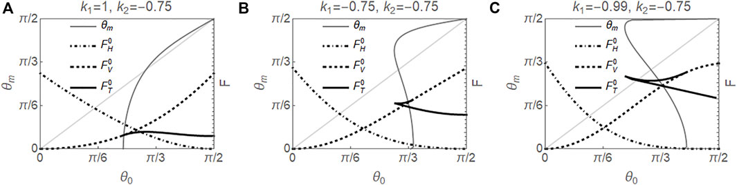
FIGURE 4. Results for k₂ = −0.75 in the absence of electric field. Left axes show solutions θ_m vs. θ₀ for the twist configuration, and right axes show the scaled energies for splay $(F_H^0)$, bend $(F_V^0)$, and twist $(F_T^0)$ configurations vs. θ₀. For (A) k₁ = 1, there is a second order transition from bend to twist. For (B) k₁ = −0.75, there is a first order transition from bend to twist. For (C) k₁ = −0.85, the bistable region of θ₀ gets larger than that of k₁ = −0.75.

As can be seen from Figures 2–4, the splay (H) is always a locally stable configuration and has lower energy than those of the bend (V) and twist (T) at large pretilt angles. However, the system will not automatically be in the global minimum energy state. In fact, the configuration the system adopts depends sensitively on the initial condition. If an electric field is applied to align the directors in the interior to be parallel to the plates, then after the field is removed, the system will relax to the splay (H) configuration. On the other hand, if the field is to align the directors parallel to the normal direction, then after the field is turned off, the system will relax to either bend (V) or twist (T) configuration, depending on which attraction basin that initial high energy configuration resides in.

Figure 5 shows the phase diagrams for the stable bend (V) and twist (T) configurations in terms of k₁ and θ₀ for those three values of k₂. As noted above, the bend (V) or twist (T) configuration can only be observed if the system is relaxed from an excited state with the director field in proximity of homeotropic configuration, where the directors in the interior of the cell are perpendicular to the plates. Dashed curves indicate the spontaneous second order transitions as θ₀ varies, and thick solid curves indicate spinodal lines where the bend (V) configuration loses its local stability at the upper solid curve, and the twist (T) configuration loses its local stability at the lower solid curve. The regions enclosed by these solid curves contain one locally stable bend (V) and one locally stable twist (T) configuration. The thin curves in the bistable region mark the first order transitions where the free energies of the bend (V) and twist (T) are the same. Specifically, for k₂ = 0, containing the one constant approximation case, if k₁ > 0, there is a second order transition from bend to twist as θ₀ increases, whereas equilibrium twist configuration does not exist if k₁ < 0, as shown in Figure 5A. For k₂ = −0.5, the transition from bend to twist is second order for larger k₁ and becomes first order for smaller k₁, as shown in Figure 5B. The transition for k₂ = −0.75 is similar to that of k₂ = −0.5, except that the bistable region becomes much larger and shifts to smaller values of θ₀. Those results are consistent with the fact that the twist distortion is energetically cheap for small k₂, and the bend distortion is expensive for large k₁ and θ₀.

FIGURE 5

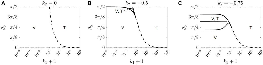
FIGURE 5. Phase diagrams for locally stable bend and twist configurations in the absence of electric field in terms of k₁ and θ₀ for (A) k₂ = 0, (B) k₂ = −0.5, and (C) k₂ = −0.75. The second order transitions between bend and twist configurations are represented by dashed curves. The thick solid curves are spinodal lines where the bend (V) configuration loses its local stability at the upper solid curve, and the twist (T) configuration loses its local stability at the lower solid curve. The thin curves in between mark the first order transitions where the free energy of the bend (V) is the same as that of the twist (T). These phases are observable when the LC director field is relaxed from the homeotropic configuration where interior directors are aligned perpendicular to the plates. We note that splay is always a locally stable configuration, not shown in the phase diagrams, and can be realized when the system is relaxed from the homogeneous configuration where the interior directors are aligned parallel to the plates.

Porte and Jadot (Porte and Jadot, 1978) have considered the transition between twist and bend configurations of a twisted nematic liquid crystal cell induced by the pretilt angle at bounding surfaces. When the overall twist is π, it is equivalent to the pi-cell. The authors concluded that the order of transition between bend and twist depends only on the value of k₂. In particular, they claimed that the second order transition occurs for k₂ ≤ −0.5 and first order transition occurs for k₂ > − 0.5. As we just showed, our results are in contrast with those in (Porte and Jadot, 1978); the order of transition between the bend and twist indeed depends on both values of k₁ and k₂. Specifically, second order transition occurs for larger values of k₁ for all values of k₂, and first order transition occurs for smaller values of k₁ for k₂ = −0.5, −0.75.

4 Solutions under an electric field

In this section, we study the configuration transitions for a nematic pi-cell under an electric field. As we shall show in Section 4.1, the symmetric splay configuration becomes asymmetric splay as α increases, and in Section 4.2, the bend configuration becomes twist as α decreases, and vice versa.

4.1 Splay configurations

When an electric field is applied perpendicular to the pi-cell with ɛ_a < 0 and initial splay configuration, the splay configuration is reinforced as the field tends to align the director parallel with the bounding plates, hence θ(z) approaches π/2 everywhere in the cell and remains monotonic, as illustrated by the dashed curve in Figure 6A. However, if ɛ_a > 0, the field tends to align the director parallel with the cell normal, and θ(z) tends to either 0 or π everywhere in the cell. Beyond a threshold voltage α_cs, θ(z) loses its monotonicity and two nonmonotonic splay configurations are found: a symmetric splay (Hs*) and an asymmetric splay (Ha), illustrated by the dotted and solid curves in Figure 6A, respectively. We remark that the symmetric configuration Hs* is unstable to Ha under an asymmetric perturbation of the solution. Figure 6B shows the corresponding electric field variations in the cell for each configuration in A. We note that the relation between the magnitude of the electric field and tilt angle is given in Eq. 16.

FIGURE 6

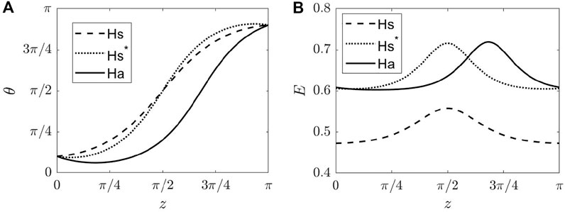
FIGURE 6. Representative solutions for splay configurations in a pi-cell under an electric field, obtained with Matlab numerical package BVP5c. The (A) tilt angle θ and (B) corresponding nondimensionalized electric field are shown. The dashed curve for Hs represents the solution for α = 2.5, and the dotted and solid curves represent the symmetric (Hs*) and asymmetric splay (Ha) configurations when α = 4, respectively. Parameters used are k₁ = k₂ = 0, θ₀ = π/10, γ = 0.2, α_cs ≈ 2.9.

The threshold voltage can be found by recognizing that at α_cs, θ′(0) = θ′(π) = 0. Then from Eqs. 17, 23, 24, we obtain

${\alpha }_{cs}={\left(\frac{1}{\pi }{\int }_{{\theta }_0}^{\pi -{\theta }_0}\frac{1}{{\gamma }^{-1}+{\cos }^2\theta }\sqrt{\frac{f\left(\theta \right)}{\frac{1}{{\gamma }^{-1}+{\cos }^2\theta }-\frac{1}{{\gamma }^{-1}+{\cos }^2{\theta }_0}}}d\theta \right)}^2.(54)$

The singularity in the integrand at θ₀ in Eq. 54 can be removed by the change of variables, sin λ cos θ₀ = cos θ, which gives

${\alpha }_{cs}={\left(\frac{2}{\pi }\sqrt{{\gamma }^{-1}+{\cos }^2{\theta }_0}{\int }_0^{\pi /2}\frac{\sqrt{1+k_1\left(1-{\sin }^2\lambda {\cos }^2{\theta }_0\right)}}{\sqrt{\left({\gamma }^{-1}+{\sin }^2\lambda {\cos }^2{\theta }_0\right)}\sqrt{1-{\sin }^2\lambda {\cos }^2{\theta }_0}}d\lambda \right)}^2.(55)$

The threshold values α_cs in terms of θ₀ are plotted in Figure 7 for three values of k₁. The critical voltage decreases with θ₀ and increases with k₁. As θ₀ → π/2, α_cs → 1 + k₁, which is consistent with the result of $U_{0c}=\pi \sqrt{K_1/({\epsilon }_0{\epsilon }_a)}$ for the classic splay Freedericksz transition.

FIGURE 7

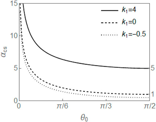
FIGURE 7. Threshold value α_cs vs. θ₀ at which splay configuration loses its monotonicity.

To study the nature of the transitions among Hs, Hs*, and Ha, we show necessary steps leading to energy calculation for each of them in detail below.

4.1.1 Monotonic splay configuration (Hs) (α < α_cs)

For small voltages α < α_cs, the splay configuration remains monotonic. Substituting Eq. 24 into Eq. 17, we have

$\pi \sqrt{\alpha }={\int }_{{\theta }_0}^{\pi -{\theta }_0}\frac{\sqrt{f\left(\theta \right)}}{\left({\gamma }^{-1}+{\cos }^2\theta \right)\sqrt{\frac{C_S}{\delta }+\frac{1}{{\gamma }^{-1}+{\cos }^2\theta }}}d\theta ,\text{\hspace{0.17em}if\hspace{0.17em}}0<\alpha <{\alpha }_{cs},(56)$

$\pi \sqrt{-\alpha }=-{\int }_{{\theta }_0}^{\pi -{\theta }_0}\frac{\sqrt{f\left(\theta \right)}}{\left({\gamma }^{-1}+{\cos }^2\theta \right)\sqrt{-\frac{C_S}{\delta }-\frac{1}{{\gamma }^{-1}+{\cos }^2\theta }}}d\theta ,\text{\hspace{0.17em}if\hspace{0.17em}}\alpha <0.(57)$

For a given θ₀ and α, we first solve C_s/δ from Eq. 56 or Eq. 57. Once C_s/δ is known, δ can be evaluated by integrating Eq. 24 from z = 0 to z = π/2 and rearranging, which gives

$|\delta |={\left(\frac{2}{\pi }{\int }_{{\theta }_0}^{\pi /2}\frac{\sqrt{f\left(\theta \right)}}{\sqrt{\left|\frac{C_S}{\delta }+\frac{1}{{\gamma }^{-1}+{\cos }^2\theta }\right|}}d\theta \right)}^2.(58)$

Now that C_s is known, the energy for the monotonic splay configuration is then $F_{Hs}=\frac{K_{3}A{\pi }^2}{2d}{C}_s$.

4.1.2 Symmetric splay configuration (Hs*) (α > α_cs)

For voltages above the critical value α > α_cs, θ(z) is no longer monotonic. Assuming the solution continues to have the mirror symmetry, θ(π − z) = π − θ(z), then we only need to focus on the bottom half. In this half of the cell, θ(z) first decreases in $(0,\widehat{z})$ and reaches its local minimum θ_m at $z=\widehat{z}$, that is,

$\theta \left(\widehat{z}\right)={\theta }_m,{\theta }^{\prime }\left(\widehat{z}\right)=0,(59)$

and increases back in $(\widehat{z},\pi /2)$. With Eqs 59, 23, one gets $C_s=-\frac{\delta }{{\gamma }^{-1}+{\cos }^2{\theta }_m}$, and Eq. 24 becomes

$dz=\pm \sqrt{\frac{f\left(\theta \right)}{\frac{\delta }{{\gamma }^{-1}+{\cos }^2\theta }-\frac{\delta }{{\gamma }^{-1}+{\cos }^2{\theta }_m}}}d\theta ,(60)$

where the plus sign is taken for $z\in (\widehat{z},\pi /2)$, and the minus sign is taken for $z\in (0,\widehat{z})$. Substituting Eq. 60 into Eq. 17 and using the transformation sin λ cos θ_m = cos θ, we get

$\pi \sqrt{\alpha }=2\sqrt{{\gamma }^{-1}+{\cos }^2{\theta }_m}\times \left({\int }_{{\lambda }_0}^{\pi /2}+{\int }_0^{\pi /2}\frac{\sqrt{1+k_1\left(1-{\sin }^2\lambda {\cos }^2{\theta }_m\right)}}{\sqrt{\left({\gamma }^{-1}+{\sin }^2\lambda {\cos }^2{\theta }_m\right)}\sqrt{1-{\sin }^2\lambda {\cos }^2{\theta }_m}}d\lambda \right),(61)$

where sin λ₀ cos θ_m = cos θ₀. In Eq. 61 and similar ones hereinafter, both integrals on the right hand sides share the same integrand. The integrand in the first integral is omitted to make the presentation compact.

For given θ₀ and α, θ_m is determined from Eq. 61. We note the right hand side of Eq. 61 is a continuous decreasing function of θ_m in (0, θ₀). This guarantees the existence of the solution θ_m for each α > α_cs. Once θ_m is known, δ can be calculated by integrating Eq. 60 from z = 0 to z = π/2 and rearranging to get

$\begin{array}{ll}\hfill \delta & =\frac{4\left({\gamma }^{-1}+{\cos }^2{\theta }_m\right)}{{\pi }^2}\hfill \\ \hfill & \times {\left({\int }_{{\lambda }_0}^{\pi /2}+{\int }_0^{\pi /2}\frac{\sqrt{1+k_1\left(1-{\sin }^2\lambda {\cos }^2{\theta }_m\right)}\sqrt{\left({\gamma }^{-1}+{\sin }^2\lambda {\cos }^2{\theta }_m\right)}}{\sqrt{1-{\sin }^2\lambda {\cos }^2{\theta }_m}}d\lambda \right)}^2.\hfill \end{array}(62)$

The energy is then given by

$F_{H{s}^{\ast }}=\frac{K_{3}A{\pi }^2}{2d}{C}_S=-\frac{K_{3}A{\pi }^2}{2d}\frac{\delta }{{\gamma }^{-1}+{\cos }^2{\theta }_m}.(63)$

4.1.3 Asymmetric splay configuration (Ha) (α > α_cs)

Since the asymmetric splay configuration is nonmonotonic, the corresponding θ(z) necessarily possesses an interior local extremum. In fact, there is one such configuration where θ₁(z) possesses a local minimum, and another where θ₂(z) possesses a local maximum. We focus on the first configuration as the other is related by θ₁(π − z) = π − θ₂(z).

Now since θ(z) has a local minimum, it follows that θ(z) decreases from z = 0 and reaches its local minimum θ_m at $z=\tilde{z}$, that is

$\theta \left(\tilde{z}\right)={\theta }_m,{\theta }^{\prime }\left(\tilde{z}\right)=0,(64)$

and increases back for $z\in (\tilde{z},\pi )$. With Eqs 64, 23, one gets $C_s=-\frac{\delta }{{\gamma }^{-1}+{\cos }^2{\theta }_m}$, and Eq. 24 becomes

$dz=\pm \sqrt{\frac{f\left(\theta \right)}{\frac{\delta }{{\gamma }^{-1}+{\cos }^2\theta }-\frac{\delta }{{\gamma }^{-1}+{\cos }^2{\theta }_m}}}d\theta ,(65)$

where the plus sign is taken for $z\in (\tilde{z},\pi )$, and the minus sign is taken for $z\in (0,\tilde{z})$. Substituting Eq. 65 into Eq. 17 and using the transformation sin λ cos θ_m = cos θ gives

$\pi \sqrt{\alpha }=\sqrt{{\gamma }^{-1}+{\cos }^2{\theta }_m}\times \left({\int }_{{\lambda }_0}^{\pi /2}+{\int }_{-{\lambda }_0}^{\pi /2}\frac{\sqrt{1+k_1\left(1-{\sin }^2\lambda {\cos }^2{\theta }_m\right)}}{\sqrt{\left({\gamma }^{-1}+{\sin }^2\lambda {\cos }^2{\theta }_m\right)}\sqrt{1-{\sin }^2\lambda {\cos }^2{\theta }_m}}d\lambda \right),(66)$

where sin λ₀ cos θ_m = cos θ₀.

Given θ₀ and α, we first solve θ_m from Eq. 66. Similar to the case of the nonmonotonic symmetric Hs*, the right hand side of Eq. 66 is a continuous decreasing function of θ_m in (0, θ₀), which guarantees the existence of the solution θ_m for any α > α_cs. Once θ_m is known, δ can be evaluated by integrating Eq. 65 from z = 0 to z = π and rearranging for

$\begin{array}{ll}\hfill \delta & =\frac{{\gamma }^{-1}+{\cos }^2{\theta }_m}{{\pi }^2}\hfill \\ \hfill & \times {\left({\int }_{{\lambda }_0}^{\pi /2}+{\int }_{-{\lambda }_0}^{\pi /2}\frac{\sqrt{1+k_1\left(1-{\sin }^2\lambda {\cos }^2{\theta }_m\right)}\sqrt{\left({\gamma }^{-1}+{\sin }^2\lambda {\cos }^2{\theta }_m\right)}}{\sqrt{1-{\sin }^2\lambda {\cos }^2{\theta }_m}}d\lambda \right)}^2,\hfill \end{array}(67)$

and the energy for the asymmetric splay configuration can be evaluated by the same equation as Eq. 63.

The results in Sections 4.1.1 4.1.2, and 4.1.3 are exemplified in Figure 8, which shows the representative minimum tilt angles θ_m and associated energies for Hs, Hs*, and Ha for one specific set of parameters. It clearly shows that the Ha state branches off from the Hs state as a second order transition at α_cs and possesses lower energy than that of the Hs* configuration. We note that the results are independent of values of k₂.

FIGURE 8

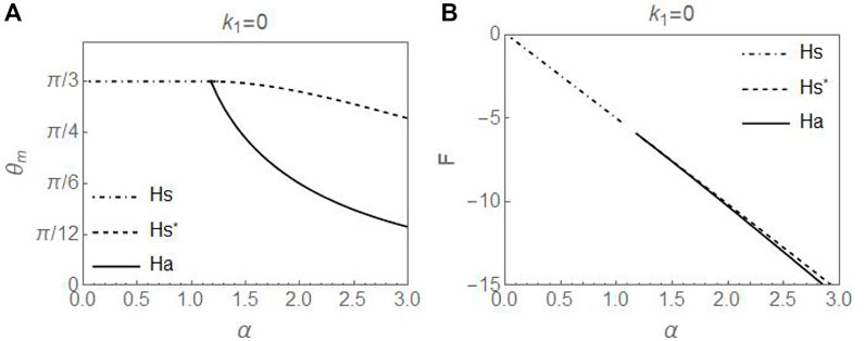
FIGURE 8. The (A) minimum values θ_m and (B) associated energies of symmetric monotonic (Hs), symmetric nonmonotonic (Hs*), and asymmetric (Ha) splay configurations as functions of α. Parameters used are k₁ = 0, θ₀ = π/3, γ = 0.2.

4.2 Bend and twist configurations

We have shown in Section 3 that bend and twist configurations can be transitioned into one another by varying the boundary pretilt angles, and the transitions can be either first order or second order depending on the material parameters. In this section, we show how the electric field affects both configurations and the transitions between them.

When an electric field is applied across the pi-cell with initial bend configuration and the nematic has ɛ_a > 0, the bend configuration is reinforced, since the field tends to align the director parallel to the field direction, and θ(z) remains monotonic, as illustrated by the dashed curve in Figure 9A. However, if ɛ_a < 0, the field tends to align the director parallel with the bounding plates, and θ(z) increases in its magnitude as voltage increases. Here, we consider two scenarios: first, we confine the directors lying in the xz − plane; second, the directors are allowed to have nonvanishing out-of-plane components.

FIGURE 9

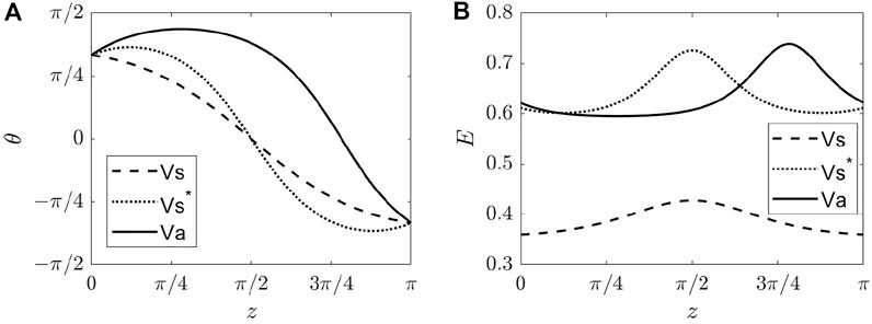
FIGURE 9. Representative solutions for bend configurations in a pi cell for LCs with ɛ_a < 0. The (A) tilt angle θ(z) and (B) corresponding nondimensionalized electric field are shown. The dashed curve for symmetric bend configuration (Vs) is obtained when α = −1.5, and the dotted and solid curves for the symmetric (Vs*) and asymmetric (Va) bend configurations are obtained when α = −4. Parameters used are k₁ = k₂ = 0, θ₀ = π/3, γ = −0.2, α_cb ≈ − 2.

In the first scenario, the bend configuration loses its monotonicity beyond a threshold voltage. Similar to the case of splay configuration, we found a symmetric (Vs*) and an asymmetric (Va) nonmonotonic equilibrium bend configuration, as shown as the dotted and solid curves in Figure 9A. Further calculations show the asymmetric one having less energy than that of the symmetric. We omit the detailed calculations here as the analyses are identical to the case of splay configurations aside from the different boundary conditions and the nonmonotonic solution existing for ɛ_a < 0.

The threshold α_cb can be found by recognizing that at α = α_cb, θ′(0) = θ′(π) = 0. Using Eqs 17, 30 and 31, and the transformation cos λ sin θ₀ = sin θ, the threshold value α_cb is given by

${\alpha }_{cb}=-{\left(\frac{2}{\pi }\sqrt{-{\gamma }^{-1}-{\cos }^2{\theta }_0}{\int }_0^{\pi /2}\frac{\sqrt{1+k_1{\cos }^2\lambda {\sin }^2{\theta }_0}}{\sqrt{-{\gamma }^{-1}-1+{\cos }^2\lambda {\sin }^2{\theta }_0}\sqrt{1-{\cos }^2\lambda {\sin }^2{\theta }_0}}d\lambda \right)}^2.(68)$

The threshold values α_cb in terms of θ₀ are plotted in Figure 10 for three values of k₁. The critical voltage increases with θ₀ and with k₁. As θ₀ → 0, α_cb → −1, which is independent of k₁. This is consistent with the critical voltage $U_{0c}=\pi \sqrt{K_3/|{\epsilon }_0{\epsilon }_a|}$ for classic bend Freederickz transition.

FIGURE 10

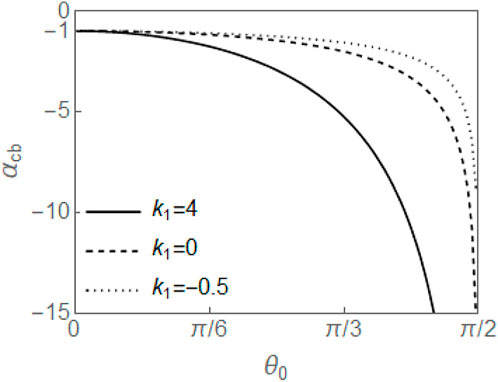
FIGURE 10. Threshold value α_cb vs. θ₀ at which bend configuration loses its monotonicity.

In the second scenario, the bend configuration is subject to out-of-plane perturbation. For sufficiently high voltages, the bend becomes twist. To study the configuration transition between bend and twist as α varies, we carry out the calculations for the twist configurations under an electric field as described in Section 2.2.3 and find the critical voltage when θ_m becomes zero, an indicator for the transition from twist to bend. Figure 11 shows three representative solutions of (A) θ(z), (B) ϕ(z), and (C) the magnitude of the electric field of twist configurations in a pi-cell for the cases α = 0, α > 0, and α < 0. If ɛ_a < 0, the tilt angle increases with α, and the configuration remains as twist, shown as dashed curves. However if ɛ_a > 0, the tilt angle decreases with α. At a threshold voltage, depicted by the dotted curve, the tilt angle at the midplane θ_m goes to 0, and ϕ approaches a step function with ϕ = 0 at lower half and ϕ = π at the upper half of the cell. It follows that the twist configuration becomes bend.

FIGURE 11

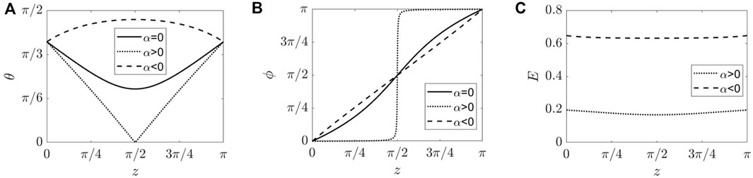
FIGURE 11. Representative solutions for twist configurations in a pi-cell with α = 0, 0.32, and − 4. The (A) tilt angle θ(z), (B) corresponding azimuthal angle ϕ(z), and (C) corresponding nondimensionalized electric field are shown. Parameters used are k₁ = 1, k₂ = 0, θ₀ = 1.2, |γ| = 0.2.

Figure 12 shows the phase diagrams for stable bend and twist configurations in terms of θ₀ and α with three representative sets of material parameters. Figure 12A with k₁ = k₂ = 0, Figure 12B with k₁ = −0.1, k₂ = −0.5, and Figure 12C with k₁ = k₂ = −0.75, separately represent the parameter sets where there is no transition, a second order transition, and a first order transition from bend to twist configurations as θ₀ varies in the absence of an electric field. In Figure 12C, there are two critical boundary pretilt angles at α = 0 (also shown in Figure 4B), with the smaller one corresponding to the critical θ₀ below which the twist solution loses its local stability, and the larger one corresponding to the critical θ₀ beyond which the bend solution loses its local stability. In between these two angles, both bend and twist are locally stable. The bistable region shrinks as α decreases and second order transition takes over. In all three cases, the threshold voltage for the transition from bend to twist decreases with θ₀, whereas the threshold voltage for the transition from twist to bend increases with θ₀.

FIGURE 12

FIGURE 12. Phase diagrams for locally stable bend and twist configurations in terms of θ₀ and α for (A) k₁ = k₂ = 0, (B) k₁ = −0.1, k₂ = −0.5, and (C) k₁ = −0.75, k₂ = −0.75. Dashed curves indicate that the transition between bend (V) and twist (T) configurations is second order. Solid curves indicate the spinodal lines where the bend and twist lose their local stabilities at the lower and upper solid curves, respectively, and in between the two solid curves are two locally stable states Vs, and T.

We remark that the transitions from monotonic bend to twist always occur at an α_ct ≥ −1, as shown in Figure 12, whereas the transitions from monotonic bend to nonmonotonic bend always occur at α_cb ≤ −1, as shown in Figure 10. Therefore, the transition from bend to twist occurs at a lower voltage, thus the latter transition is preempted and typically not observable.

5 Summary

In this work, we have conducted a detailed parameter study of equilibrium states in a nematic pi-cell under an electric field applied perpendicular to the bounding plates. The distortion of liquid crystals is modeled with the one-dimensional Oseen-Frank director model, and the effect of director distortion on the electric field has been incorporated.

In the absence of electric field, the equilibrium splay, bend, and twist configurations all possess certain symmetries with respect to the midplane. The splay configuration is always locally stable. Bend is always stable for small θ₀, the pretilt angle at the boundary. As θ₀ increases, bend is likely to lose its stability to twist if k₂ is small, where twist configuration is energetically cheap, or if k₁ is large, where the energy cost for the bend configuration is large. A range of θ₀ where both bend and twist are locally stable is found for small k₁ and k₂ ≤ −0.5. Our results are in contrast with those in (Porte and Jadot, 1978), where the authors reported that the second order transition between bend and twist occurs for k₂ ≤ −0.5, and first order transition occurs for k₂ > − 0.5, whereas, we have shown that second order transition occurs for larger values of k₁ and for all k₂ and first order transition occurs for smaller values of k₁ and k₂.

When a voltage difference is applied perpendicular to the pi-cell, the configuration transitions depend on the initial configuration and the sign of the dielectric anisotropy. Starting from the splay configuration and ɛ_a > 0, the symmetric splay continuously transitions to asymmetric splay at a threshold voltage. If the initial configuration is bend (twist) and ɛ_a < 0 (ɛ_a > 0), then bend (twist) configuration becomes twist (bend) for sufficiently high voltages. The transition between bend and twist is likely to be second order for large values of k₁ and for small θ₀ and could be first order for small values of k₁ and k₂ and large θ₀.

Our results based on the one-dimensional Oseen-Frank director model cannot describe the transitions between splay and bend/twist configurations as the switching among those topologically distinct configurations would require at least a two-dimensional model or a tensor description (Amoddeo and Barberi, 2021) of orientation field where the disclinations are allowed. With that said, our results will help to predict the equilibrium configurations after the voltage is removed and the voltage required to ensure that an asymmetric splay, bend or twist configuration is achieved given the material parameters and the pretilt angle at the boundary.

Data availability statement

The original contributions presented in the study are included in the article/supplementary material, further inquiries can be directed to the corresponding author.

Author contributions

The authors contributed equally to the manuscript.

Conflict of interest

The handling Editor HY declared a shared affiliation with the authors at the time of review.

The remaining author declares that the research was conducted in the absence of any commercial or financial relationships that could be construed as a potential conflict of interest.

Publisher’s note

All claims expressed in this article are solely those of the authors and do not necessarily represent those of their affiliated organizations, or those of the publisher, the editors and the reviewers. Any product that may be evaluated in this article, or claim that may be made by its manufacturer, is not guaranteed or endorsed by the publisher.

References

Amoddeo, A., and Barberi, R. (2021). Phase diagram and order reconstruction modeling for nematics in asymmetric pi-cells. Symmetry 13 (11), 2156. doi:10.3390/sym13112156

CrossRef Full Text | Google Scholar

Berreman, D. W., and Heffner, W. R. (1980). New bistable cholesteric liquid crystal display. Appl. Phys. Lett. 37 (1), 109–111. doi:10.1063/1.91680

CrossRef Full Text | Google Scholar

Berreman, D. W., and Heffner, W. R. (1981). New bistable liquid crystal twist cell. J. Appl. Phys. 52 (4), 3032–3039. doi:10.1063/1.329049

CrossRef Full Text | Google Scholar

Bos, P. J., and Beran, K. R. (1984). The pi-cell: A fast liquid-crystal optical-switching device. Mol. Cryst. Liq. Cryst. 113 (1), 329–339. doi:10.1080/00268948408071693

CrossRef Full Text | Google Scholar

Boyd, G. D., Cheng, J., and Ngo, P. D. T. (1980). Liquid crystal orientational bistability and nematic storage effects. Appl. Phys. Lett. 36 (7), 556–558. doi:10.1063/1.91578

CrossRef Full Text | Google Scholar

Bryan-Brown, G. P., Towler, M. J., Bancroft, M. S., and McDonnell, D. G. (1994). “October. Bistable nematic alignment using bigratings,” in Proceedings of International Display Research Conference, 209–212.

Google Scholar

Deuling, H. J. (1972). Deformation of nematic liquid crystals in an electric field. Mol. Cryst. Liq. Cryst. 19 (2), 123–131. doi:10.1080/15421407208083858

CrossRef Full Text | Google Scholar

Dozov, I., and Durand, G. (1998). Surface controlled nematic bistability: From surface anchoring bifurcation to fast displays with video compatibility. Liq. Cryst. Today 8 (2), 1–7. doi:10.1080/13583149808047702

CrossRef Full Text | Google Scholar

Ericksen, J. L. (1966). Inequalities in liquid crystal theory. Phys. Fluids. 9 (6), 1205–1207. doi:10.1063/1.1761821

CrossRef Full Text | Google Scholar

Frank, F. C. (1958). I. Liquid crystals on the theory of liquid crystals. Discuss. Faraday Soc. 25, 19–28. doi:10.1039/df9582500019

CrossRef Full Text | Google Scholar

Gartland, E. C. (2020). Forces and variational compatibility for equilibrium liquid crystal director models with coupled electric fields. Continuum Mechanics and Thermodynamics, 32 (6), 1559–1593.

CrossRef Full Text | Google Scholar

Haller, I. (1972). Elastic constants of the nematic liquid crystalline phase of p-Methoxybenzylidene-p-n-Butylaniline (MBBA). J. Chem. Phys. 57 (4), 1400–1405. doi:10.1063/1.1678416

CrossRef Full Text | Google Scholar

Jhun, C. G., Chen, C. P., Lee, U. J., Lee, S. R., Yoon, T. H., and Kim, J. C. (2006). Tristate liquid crystal display with memory and dynamic operating modes. Appl. Phys. Lett. 89 (12), 123507. doi:10.1063/1.2354430

CrossRef Full Text | Google Scholar

Kim, J. H., Yoneya, M., Yamamoto, J., and Yokoyama, H. (2001). Surface alignment bistability of nematic liquid crystals by orientationally frustrated surface patterns. Appl. Phys. Lett. 78 (20), 3055–3057. doi:10.1063/1.1371246

CrossRef Full Text | Google Scholar

Lagerwall, S. T. (1999). Ferroelectric and antiferroelectric liquid crystals. Weinheim: Wiley VCH.

Google Scholar

Leger, L. (1972). Static and dynamic behaviour of walls in nematics above a Freedericks transition. Solid State Commun. 11 (11), 1499–1501. doi:10.1016/0038-1098(72)90508-x

CrossRef Full Text | Google Scholar

Lin, G. J., Chen, T. J., Lin, B. R., Liao, H. I., Chang, Y., Wu, J. J., et al. (2015). Effects of pretilt angle on electro-optical properties of optically compensated bend liquid crystal devices with a mixed polyimide alignment layer. J. Disp. Technol. 12 (3), 302–308. doi:10.1109/jdt.2015.2502722

CrossRef Full Text | Google Scholar

Oseen, C. W. (1933). The theory of liquid crystals. Trans. Faraday Soc. 29, 883. doi:10.1039/tf9332900883

CrossRef Full Text | Google Scholar

Porte, G., and Jadot, J. P. (1978). A phase transition-like instability in static samples of twisted nematic liquid crystal when the surfaces induce tilted alignments. J. Phys. Fr. 39 (2), 213–223. doi:10.1051/jphys:01978003902021300

CrossRef Full Text | Google Scholar

Scheffer, T. J. (1978). Distorted twisted nematic liquid-crystal structures in zero field. J. Appl. Phys. 49, 5835–5842. doi:10.1063/1.324600

CrossRef Full Text | Google Scholar

Wu, J. J., Hu, S. S., Hsu, C. C., Chen, T. J., and Lee, K. L. (2012). Electro optical characteristics of high-pretilt twisted liquid crystal pi-cells. Appl. Phys. Express 6 (1), 012201. doi:10.7567/apex.6.012201

CrossRef Full Text | Google Scholar

Yang, D. K., West, J. L., Chien, L. C., and Doane, J. W. (1994). Control of reflectivity and bistability in displays using cholesteric liquid crystals. J. Appl. Phys. 76 (2), 1331–1333. doi:10.1063/1.358518

CrossRef Full Text | Google Scholar

Yu, X. J., and Kwok, H. S. (2004). Bistable bend-splay liquid crystal display. Appl. Phys. Lett. 85 (17), 3711–3713. doi:10.1063/1.1810215

CrossRef Full Text | Google Scholar

Zhou, X., Qin, G., Xu, X., and Yang, D. K. (2017). P-161: Reverse OCB liquid crystal display. SID Symposium Dig. Tech. Pap. 48 (1), 1888–1891. doi:10.1002/sdtp.12067

CrossRef Full Text | Google Scholar