Theoretical and experimental results on time-series representations of polynomials

This study considers time-series representations of polynomials. Often in data modelling and many other applications, accurate estimations of the degree of a polynomial, of the noise standard deviation, and of the coefficient of the highest degree of a polynomial are useful in detection, estimation, and prediction. The major contributions of this paper can be found in the original research offering novel theoretical and experimental results. The theoretical results include an alternative proof of the qth order AR time-series representation, with a constant, of a polynomial of degree q, an alternative proof of the (q + 1)-th order AR time-series representation, without a constant, of a polynomial of degree q, as well as generalized equations (valid for a polynomial of an arbitrary degree) for reduced variance estimation of the polynomial coefficient corresponding to the highest degree. The experimental investigations are the most comprehensive so far, in that they use well over 35 times more realisations than before, use a greater variety of noisy data (Gaussian, Uniform, and Exponential noise), and use a larger range of polynomial degrees as well as of noise standard deviations than before. Experimental results on estimations of the degree of a polynomial, of the noise standard deviation, and of the polynomial coefficient corresponding to the highest degree using seven methods (AIC, AICc, GIC, BIC, Chi-square, F-distribution, and PTS2) are presented. Results indicate clearly that PTS2 performs the best.

1 Introduction

The representation of a polynomial of an arbitrary degree with an AR model of the same order with a constant term was presented in (Nandi, 2020a), in which all the coefficients of the AR model were explicitly derived independent of the polynomial coefficients and the constant term was also derived, containing the degree of the polynomial and the polynomial coefficient corresponding to the highest degree. Inspired by this research, a completely original paradigm for polynomial degree estimation (PTS1) was introduced (Nandi, 2020b). Until recently, the estimation of the degree of a polynomial has been achieved using many model order selection techniques. Existing techniques select a model, which includes both the degree and all coefficients of a polynomial, from a set of candidate models which are then fitted to the data. Instead, the novel paradigm in (Nandi, 2020b) utilizes the variance of the estimated constant term in the corresponding AR representation to estimate the degree of a polynomial, without requiring either the estimation or the knowledge of any polynomial coefficients; this is fundamentally different from what have been practised in the past.

Following the aforementioned two studies, a third study was reported (Nandi, 2021), which adopted the novel paradigm and proposed a novel method (PTS2) to estimate the degree of a polynomial. Using the estimated degree, it proposed a method to estimate the additive noise standard deviation and another method to estimate the value of the polynomial coefficient corresponding to the highest degree. Novel applications of these studies are being developed. In (Sivaraman et al., 2024), authors wrote, “Nandi’s seminal works (Nandi, 2020a; Nandi, 2020b; Nandi, 2021) have significantly advanced our understanding of polynomial and time-series representations, model-order selection, and noise power estimation, forming the basis for the current study”. They presented a novel approach for adaptive non-linear state estimation in a modified autoregressive time series with fixed coefficients. Their proposed adaptive polynomial Kalman filter (APKF) has been claimed to be superior in estimating the state of the true system compared with the traditional Kalman filters. In (Zhang et al., 2025), the authors developed a broken-track association method for multi-target tracking. They utilise the results from Stone-Weiestrass theorem that any time-varying motion of a maneuvering target can be described well by a high-order polynomial (You et al., 2019). Hence, instead of directly using the polynomial model, which requires the knowledge of the unknown polynomial coefficients, they chose to adopt the corresponding time-series representation.

This paper contains original research, including novel theoretical and experimental results. Section 2 contains theoretical results, including 1) an alternative proof of the qth order AR time-series representation, with a constant, of a polynomial of degree q, 2) an alternative proof of the (q + 1)-th order AR time-series representation, without a constant, of a polynomial of degree q, as well as 3) generalized equations, valid for a polynomial of an arbitrary degree, for reduced variance estimation of the polynomial coefficient corresponding to the highest degree. Section 3 provides details of the experimental investigations and novel comprehensive results from noisy data using additive Gaussian, Uniform, and Exponential noise. Finally, the paper is concluded in Section 4.

2 Theoretical results

This section is comprised of three subsections. The first subsection provides an alternative proof of the fact that every polynomial of degree q can be represented by an autoregressive (AR) time-series of order q with a constant term µ, such that the time-series coefficients are given by ${\left(-1\right)}^{i+1}$ $\left(\begin{array}{l}q\\ i\end{array}\right)$, for $i=1,2,\dots ,q$ and $\mathrm{\mu }=c\left(q\right)T^q\left(q!\right)$, T being the sampling period. The second subsection provides a proof of an alternative time-series representation that every polynomial of degree q can be represented by an autoregressive (AR) time-series of order (q + 1) without any constant term, such that the time-series coefficients are given by ${\left(-1\right)}^{i+1}$ $\left(\begin{array}{l}q+1\\ i\end{array}\right)$, for $i=1,2,\dots ,\left(q+1\right)$. The third subsection provides new generalized theoretical relations for obtaining reduced variance estimation of the polynomial coefficient corresponding to the highest degree.

2.1 An alternative proof of the time-series representation with a constant term

A polynomial of degree q in a continuous variable t (let us say that it is time) can be written as

$\mathit{y}\left(\mathit{t}\right)={\displaystyle \sum _{\mathit{i}=\mathbf{0}}^{\mathit{q}}}\mathit{c}\left(\mathit{i}\right){\mathit{t}}^{\mathit{i}}(1)$

If the continuous variable, t, is uniformly sampled (or discretized), it can be represented as $t=nT$, where n is an integer and T is the sampling period. In this scenario, the above equation can be rewritten as $y\left(nT\right)={\displaystyle {\sum }_{i=0}^q}c\left(i\right){\left(nT\right)}^i$. For simplicity in notations and without the loss of any generality, this can be re-written as

$\mathit{y}\left(\mathit{n}\right)={\displaystyle \sum _{\mathit{i}=\mathbf{0}}^{\mathit{q}}}\mathit{c}\left(\mathit{i}\right){\mathit{n}}^{\mathit{i}}(2)$

The new value of $c\left(i\right)$ in Equation 2 is the old value of $c\left(i\right)$ multiplied by $T^i$. In (Nandi, 2020a) it was proven that all noise-free data from uniformly sampled polynomials of finite degree q can be represented by an autoregressive “time-series” model of order q such that

$\mathit{y}\left(\mathit{n}\right)={\displaystyle \sum _{\mathit{i}=\mathbf{1}}^{\mathit{q}}}\mathit{a}\left(\mathit{i}\right)\mathit{y}\left(\mathit{n}-\mathit{i}\right)+\mathrm{\mu }$

where

$\mathrm{\mu }=\mathit{c}\left(\mathit{q}\right)\left(\mathit{q}!\right)$

and

$\mathit{a}\left(\mathit{i}\right)={\left(-\mathbf{1}\right)}^{\mathit{i}+\mathbf{1}}\left(\begin{array}{l}\mathit{q}\\ \mathit{i}\end{array}\right),\mathit{f}\mathit{o}\mathit{r}\mathit{i}=\mathbf{1},\mathbf{2},\dots ,\mathit{q}.$

That proof in (Nandi, 2020a) was developed by 1) uniformly sampling the continuous polynomial, 2) conjecturing the time-series model, and 3) finally verifying the conjectured time-series model from first principles. From here on, T is assumed to be 1 for the sake of simplicity and without any loss of generality.

An alternative and shorter proof of the above is presented below. This follows from 1) working with a continuous polynomial, 2) differentiating this polynomial q times with respect to the continuous variable (“time”), and 3) representing the qth order derivative with linear differences using existing results. From Equation 1, we can write

$\frac{{\mathit{d}}^{\mathit{q}}\mathit{y}}{\mathit{d}{\mathit{t}}^{\mathit{q}}}=\mathit{c}\left(\mathit{q}\right)\left(\mathit{q}!\right)(3)$

Using results on backward differences from (Abramowitz and Stegun, 1972), page 877, and after some manipulations, the left-hand side of the Equation 3 can be re-written and the Equation 3 can be transformed to

$\mathit{y}\left(\mathit{n}\right)-{\displaystyle \sum _{\mathit{i}=\mathbf{1}}^{\mathit{q}}}\mathit{a}\left(\mathit{i}\right)\mathit{y}\left(\mathit{n}-\mathit{i}\right)=\mathit{c}\left(\mathit{q}\right)\left(\mathit{q}!\right)(4)$

where

$\mathit{a}\left(\mathit{i}\right)={\left(-\mathbf{1}\right)}^{\mathit{i}+\mathbf{1}}\left(\begin{array}{l}\mathit{q}\\ \mathit{i}\end{array}\right),\mathit{f}\mathit{o}\mathit{r}\mathit{i}=\mathbf{1},\mathbf{2},\dots ,\mathit{q}.$

Thus, $\mathrm{\mu }=c\left(q\right)\left(q!\right)$. Such time-series representations of polynomials of the first five degrees are given below:

$\mathit{y}\left(\mathit{n}\right)=\mathit{y}\left(\mathit{n}-\mathbf{1}\right)+\mathit{c}\left(\mathit{q}\right)\left(\mathit{q}!\right)(5)$

$\mathit{y}\left(\mathit{n}\right)=\mathbf{2}\mathit{y}\left(\mathit{n}-\mathbf{1}\right)-\mathit{y}\left(\mathit{n}-\mathbf{2}\right)+\mathit{c}\left(\mathit{q}\right)\left(\mathit{q}!\right)(6)$

$\mathit{y}\left(\mathit{n}\right)=\mathbf{3}\mathit{y}\left(\mathit{n}-\mathbf{1}\right)-\mathbf{3}\mathit{y}\left(\mathit{n}-\mathbf{2}\right)+\mathit{y}\left(\mathit{n}-\mathbf{3}\right)+\mathit{c}\left(\mathit{q}\right)\left(\mathit{q}!\right)(7)$

$\mathit{y}\left(\mathit{n}\right)=\mathbf{4}\mathit{y}\left(\mathit{n}-\mathbf{1}\right)-\mathbf{6}\mathit{y}\left(\mathit{n}-\mathbf{2}\right)+\mathbf{4}\mathit{y}\left(\mathit{n}-\mathbf{3}\right)-\mathit{y}\left(\mathit{n}-\mathbf{4}\right)+\mathit{c}\left(\mathit{q}\right)\left(\mathit{q}!\right)(8)$

$\mathit{y}\left(\mathit{n}\right)=\mathbf{5}\mathit{y}\left(\mathit{n}-\mathbf{1}\right)-\mathbf{10}\mathit{y}\left(\mathit{n}-\mathbf{2}\right)+\mathbf{10}\mathit{y}\left(\mathit{n}-\mathbf{3}\right)-\mathbf{5}\mathit{y}\left(\mathit{n}-\mathbf{4}\right)+\mathit{y}\left(\mathit{n}-\mathbf{5}\right)+\mathit{c}\left(\mathit{q}\right)\left(\mathit{q}!\right)(9)$

It should be observed that.

1) for different values of $\mathrm{\mu }$, the Equation 4 describes every polynomial of an arbitrary degree q, irrespective of the values of their coefficients,

2) for a fixed value of $\mathrm{\mu }$, the Equation 4 describes only those polynomials of degree q, with the AR constant term $\mathrm{\mu }=c\left(q\right)\left(q!\right)$, and

3) for a fixed value of $\mathrm{\mu }$, this represents every polynomial of degree q, with the polynomial coefficient corresponding to the highest degree $c\left(q\right)=\mathrm{\mu }/\left(q!\right)$. Therefore, this formulation maintains a connection between this time-series representation with a specific and infinite set of polynomials of degree q.

2.2 An alternative time-series representation without a constant term

In the previous subsection and in Nandi (2020a) it has been demonstrated that all noise-free data from uniformly sampled polynomials of finite degree q can be represented by an autoregressive “time-series” model of order q with a constant term of $\mathrm{\mu }=c\left(q\right)\left(q!\right)$, such that

$\mathit{y}\left(\mathit{n}\right)={\displaystyle \sum _{\mathit{i}=\mathbf{1}}^{\mathit{q}}}\mathit{a}\left(\mathit{i}\right)\mathit{y}\left(\mathit{n}-\mathit{i}\right)+\mathrm{\mu }$

with

$\mathrm{\mu }=\mathit{c}\left(\mathit{q}\right)\left(\mathit{q}!\right)$

and

$\mathit{a}\left(\mathit{i}\right)={\left(-\mathbf{1}\right)}^{\mathit{i}+\mathbf{1}}\left(\begin{array}{l}\mathit{q}\\ \mathit{i}\end{array}\right),\mathit{f}\mathit{o}\mathit{r}\mathit{i}=\mathbf{1},\mathbf{2},\dots ,\mathit{q}.$

In the previous subsection this was arrived at by deriving the qth order derivative of the continuous polynomial in Equation 1, which contributes the constant term. Remarkably, instead if one derives the (q+1)-th order derivative of the same continuous polynomial in Equation 1, one finds that

$\frac{{\mathit{d}}^{\mathit{q}+\mathbf{1}}\mathit{y}}{\mathit{d}{\mathit{t}}^{\mathit{q}+\mathbf{1}}}=\mathbf{0}(10)$

As in the previous subsection, using results on backward differences from (Abramowitz and Stegun, 1972), page 877, and after some manipulations, the Equation 10 can be re-written as

$\mathit{y}\left(\mathit{n}\right)-{\displaystyle \sum _{\mathit{i}=\mathbf{1}}^{\mathit{q}+\mathbf{1}}}\mathit{a}\left(\mathit{i}\right)\mathit{y}\left(\mathit{n}-\mathit{i}\right)=\mathbf{0}(11)$

where

$\mathit{a}\left(\mathit{i}\right)={\left(-\mathbf{1}\right)}^{\mathit{i}+\mathbf{1}}\left(\begin{array}{l}\mathit{q}+\mathbf{1}\\ \mathit{i}\end{array}\right),\mathit{f}\mathit{o}\mathit{r}\mathit{i}=\mathbf{1},\mathbf{2},\dots ,\left(\mathit{q}+\mathbf{1}\right).$

Such time-series representations of polynomials of the first five degrees are given by Equations 12-16 below:

$\mathit{y}\left(\mathit{n}\right)-\mathbf{2}\mathit{y}\left(\mathit{n}-\mathbf{1}\right)+\mathit{y}\left(\mathit{n}-\mathbf{2}\right)=\mathbf{0}(12)$

$\mathit{y}\left(\mathit{n}\right)-\mathbf{3}\mathit{y}\left(\mathit{n}-\mathbf{1}\right)+\mathbf{3}\mathit{y}\left(\mathit{n}-\mathbf{2}\right)-\mathit{y}\left(\mathit{n}-\mathbf{3}\right)=\mathbf{0}(13)$

$\mathit{y}\left(\mathit{n}\right)-\mathbf{4}\mathit{y}\left(\mathit{n}-\mathbf{1}\right)+\mathbf{6}\mathit{y}\left(\mathit{n}-\mathbf{2}\right)-\mathbf{4}\mathit{y}\left(\mathit{n}-\mathbf{3}\right)+\mathit{y}\left(\mathit{n}-\mathbf{4}\right)=\mathbf{0}(14)$

$\mathit{y}\left(\mathit{n}\right)-\mathbf{5}\mathit{y}\left(\mathit{n}-\mathbf{1}\right)+\mathbf{10}\mathit{y}\left(\mathit{n}-\mathbf{2}\right)-\mathbf{10}\mathit{y}\left(\mathit{n}-\mathbf{3}\right)+\mathbf{5}\mathit{y}\left(\mathit{n}-\mathbf{4}\right)-\mathit{y}\left(\mathit{n}-\mathbf{5}\right)=\mathbf{0}(15)$

$\mathit{y}\left(\mathit{n}\right)-\mathbf{6}\mathit{y}\left(\mathit{n}-\mathbf{1}\right)+\mathbf{15}\mathit{y}\left(\mathit{n}-\mathbf{2}\right)-\mathbf{20}\mathit{y}\left(\mathit{n}-\mathbf{3}\right)+\mathbf{15}\mathit{y}\left(\mathit{n}-\mathbf{4}\right)-\mathbf{6}\mathit{y}\left(\mathit{n}-\mathbf{5}\right)+\mathit{y}\left(\mathit{n}-\mathbf{6}\right)=\mathbf{0}(16)$

Although such equations have been observed before (Sivaraman et al., 2024; Zhang et al., 2025), both the above derivation and the observation of their lack of connection with any polynomial coefficient are novel. It should be noted that.

1) the Equation 11 describes every polynomial of degree q, irrespective of the values of their coefficients,

2) although the Equation 11 describes every polynomial of degree q, it has no connection with any of the coefficients in any of the polynomials of degree q, and

3) unlike the representation in the Equation 4 that can be configured to estimate the degree of a polynomial as well as the polynomial coefficient corresponding to the highest degree, the representation in the Equation 11 can be configured to estimate the degree of a polynomial but it cannot directly offer any knowledge of any of the coefficients of a polynomial.

2.3 Reduced variance estimation of the polynomial coefficient corresponding to the highest degree

It is clear from the subsection 2.1 that the value of µ contains information about the coefficient of the highest degree, q. It was discussed in (Nandi, 2020b; Nandi, 2021) that real-valued noisy data from polynomials in uniformly sampled discrete time can be represented by

$\mathit{x}\left(\mathit{n}\right)={\displaystyle \sum _{\mathit{i}=\mathbf{0}}^{\mathit{q}}}\mathit{c}\left(\mathit{i}\right){\mathit{n}}^{\mathit{i}}+\mathit{e}\left(\mathit{n}\right),(17)$

In Equation 17, $e\left(n\right)$ represents noise. In turn, the Equation 4 can be recast with known noisy data values $x\left(n\right)$ as follows

$-{\displaystyle \sum _{\mathit{i}=\mathbf{1}}^{\mathit{q}}}\mathit{a}\left(\mathit{i}\right)\mathit{x}\left(\mathit{n}-\mathit{i}\right)+\mathit{x}\left(\mathit{n}\right)=\mathrm{\mu }\left(\mathit{n},\mathit{q}\right)(18)$

where $\mathrm{\mu }\left(n,q\right)$ may depend on both n and q. Further it was demonstrated that, for the correct degree and in the presence of additive zero-mean i.i.d. Gaussian noise of variance ${\sigma }^2$, $\mathrm{\mu }\left(n,q\right)=N$ ($c\left(q\right)\left(q!\right)$, $\alpha \left(q\right)\sigma$) from Equation 18, where ${\alpha }^2\left(q\right)$ = 2, 6, 20, 70, 252, and 924 for $q$ = 1, 2, 3, 4, 5, and 6 respectively (Nandi, 2021). Therefore, while the values of µ and, in turn, $c\left(q\right)$ can be estimated in this way, their standard deviations or variances would increase with the true degree (q) and the standard deviation of the additive noise increase, if one estimates µ using Equation 18. Essentially, the variance is given by Equation 19 below

$<{\mathit{\sigma }}_{\mathit{\mu }\left(\mathit{q}\right)}{>}^{\mathbf{2}}=\left({\left(\mathbf{1}\right)}^{\mathbf{2}}+{\displaystyle \sum _{\mathit{i}=\mathbf{1}}^{\mathit{q}}}\mathit{a}{\left(\mathit{i}\right)}^{\mathbf{2}}\right){\mathit{\sigma }}^{\mathbf{2}}(19)$

A quick check of Equations 4–9 highlights the greater spread of $a\left(i\right)$ values within polynomials of degree q as well as between different degrees of polynomials. This greater spread of $a\left(i\right)$ values within polynomials of degree q gives rise to greatly increasing values of ${\alpha }^2\left(q\right)$ and, in turn, the greatly increasing values of variance or standard deviation of µ and $c\left(q\right)$.

Below we demonstrate how µ (and, in turn, $\left.c\left(q\right)\right)$ may be estimated with lower standard deviation or variance. This will not be achieved by using Equation 18 or Equation 4 directly, but by deriving new equations for µ using Equation 4, such that the spread of time-series coefficient values in the new equation is much less.

2.3.1 An example for a polynomial of degree 3

To begin with, consider the estimation of $\mathrm{\mu }$, for a time-series of order 3 corresponding to a polynomial of degree 3, using the Equation 4. In this case, one can write $\mathrm{\mu }=y\left(n\right)-3y\left(n-1\right)+3y\left(n-2\right)-y\left(n-3\right).$ Thus, the corresponding coefficients of $y\left(.\right)$ are [1, −3, 3, −1], which are fairly spread out and give rise to the variance of estimated $\mathrm{\mu }$ from Equation 4 of $20{\sigma }^2$ in the presence of additive zero-mean i.i.d. Gaussian noise of variance ${\sigma }^2$.

Now, consider the following set of four equations

$\mathrm{\mu }=\mathit{y}\left(\mathit{n}+\mathbf{3}\right)-\mathbf{3}\mathit{y}\left(\mathit{n}+\mathbf{2}\right)+\mathbf{3}\mathit{y}\left(\mathit{n}+\mathbf{1}\right)-\mathit{y}\left(\mathit{n}\right)(20)$

$\mathrm{\mu }=\mathit{y}\left(\mathit{n}+\mathbf{2}\right)-\mathbf{3}\mathit{y}\left(\mathit{n}+\mathbf{1}\right)+\mathbf{3}\mathit{y}\left(\mathit{n}\right)-\mathit{y}\left(\mathit{n}-\mathbf{1}\right)(21)$

$\mathrm{\mu }=\mathit{y}\left(\mathit{n}+\mathbf{1}\right)-\mathbf{3}\mathit{y}\left(\mathit{n}\right)+\mathbf{3}\mathit{y}\left(\mathit{n}-\mathbf{1}\right)-\mathit{y}\left(\mathit{n}-\mathbf{2}\right)(22)$

$\mathrm{\mu }=\mathit{y}\left(\mathit{n}\right)-\mathbf{3}\mathit{y}\left(\mathit{n}-\mathbf{1}\right)+\mathbf{3}\mathit{y}\left(\mathit{n}-\mathbf{2}\right)-\mathit{y}\left(\mathit{n}-\mathbf{3}\right)(23)$

Adding Equations 20–23, one obtains

$\mathbf{4}\mathrm{\mu }=\left[\mathit{y}\left(\mathit{n}+\mathbf{3}\right)-\mathbf{2}\mathit{y}\left(\mathit{n}+\mathbf{2}\right)+\mathit{y}\left(\mathit{n}+\mathbf{1}\right)\right]-\left[\mathit{y}\left(\mathit{n}-\mathbf{1}\right)-\mathbf{2}\mathit{y}\left(\mathit{n}-\mathbf{2}\right)+\mathit{y}\left(\mathit{n}-\mathbf{3}\right)\right](24)$

In Equation 24, the coefficients of $y\left(.\right)$ are [1, −2, 1, −1, 2, −1], which are less spread out. Remarkably, the variance of estimated 4 $\mathrm{\mu }$ from Equation 24 is only 12 ${\sigma }^2$ in the presence of additive zero-mean i.i.d. Gaussian noise of variance ${\sigma }^2$. It is clear therefore that the Equation 24 provides a lower variance estimate of $\mu$ than Equation 4.

The Equation 24 is based on one set of four consecutive equations, i.e., Equations 20–23. One can extend this idea further, by adding non-overlapping β sets (where β = 1, 2, 3, …) of four consecutive equations. For example, the set of four consecutive equations leading to Equation 24 corresponds to β = 1. In turn, the next set of four consecutive and non-overlapping equations corresponding to β = 2 are presented below:

$\mathrm{\mu }=\mathit{y}\left(\mathit{n}+\mathbf{7}\right)-\mathbf{3}\mathit{y}\left(\mathit{n}+\mathbf{6}\right)+\mathbf{3}\mathit{y}\left(\mathit{n}+\mathbf{5}\right)-\mathit{y}\left(\mathit{n}+\mathbf{4}\right)(25)$

$\mathrm{\mu }=\mathit{y}\left(\mathit{n}+\mathbf{6}\right)-\mathbf{3}\mathit{y}\left(\mathit{n}+\mathbf{5}\right)+\mathbf{3}\mathit{y}\left(\mathit{n}+\mathbf{4}\right)-\mathit{y}\left(\mathit{n}+\mathbf{3}\right)(26)$

$\mathrm{\mu }=\mathit{y}\left(\mathit{n}+\mathbf{5}\right)-\mathbf{3}\mathit{y}\left(\mathit{n}+\mathbf{4}\right)+\mathbf{3}\mathit{y}\left(\mathit{n}+\mathbf{3}\right)-\mathit{y}\left(\mathit{n}+\mathbf{2}\right)(27)$

$\mathrm{\mu }=\mathit{y}\left(\mathit{n}+\mathbf{4}\right)-\mathbf{3}\mathit{y}\left(\mathit{n}+\mathbf{3}\right)+\mathbf{3}\mathit{y}\left(\mathit{n}+\mathbf{2}\right)-\mathit{y}\left(\mathit{n}+\mathbf{1}\right)(28)$

Now, two ($=\mathit{\beta }$) non-overlapping sets of four equations, i.e Equations 20-23 and Equations 25-28, can be added to obtain

$\mathbf{2}\left(\mathbf{4}\mathrm{\mu }\right)=\left[\mathit{y}\left(\mathit{n}-\mathbf{1}+\mathbf{4}*\mathbf{2}\right)-\mathbf{2}\mathit{y}\left(\mathit{n}-\mathbf{2}+\mathbf{4}*\mathbf{2}\right)+\mathit{y}\left(\mathit{n}-\mathbf{3}+\mathbf{4}*\mathbf{2}\right)\right]-\left[\mathit{y}\left(\mathit{n}-\mathbf{1}\right)-\mathbf{2}\mathit{y}\left(\mathit{n}-\mathbf{2}\right)+\mathit{y}\left(\mathit{n}-\mathbf{3}\right)\right]$

Thus Equation 24 can be generalized to obtain

$\mathit{\beta }\left(\mathbf{4}\mathrm{\mu }\right)=\left[\mathit{y}\left(\mathit{n}-\mathbf{1}+\mathbf{4}\mathit{\beta }\right)-\mathbf{2}\mathit{y}\left(\mathit{n}-\mathbf{2}+\mathbf{4}\mathit{\beta }\right)+\mathit{y}\left(\mathit{n}-\mathbf{3}+\mathbf{4}\mathit{\beta }\right)\right]-\left[\mathit{y}\left(\mathit{n}-\mathbf{1}\right)-\mathbf{2}\mathit{y}\left(\mathit{n}-\mathbf{2}\right)+\mathit{y}\left(\mathit{n}-\mathbf{3}\right)\right](29)$

Therefore, the Equation 29 provides an even lower variance estimate of $\mathrm{\mu }$ than Equation 24. Now, the question is whether these ideas can be generalized for polynomials of any finite degree. If the answer is in the affirmative, the relevant equations need to be derived.

2.3.2 Generalizations for polynomials of any degree

First, it is well to understand how Equation 24 has been formed from Equations 20–23. The coefficients of $y\left(.\right)$ in Equation 24 has been obtained by adding all relevant coefficients of $y\left(.\right)$ along the diagonal line going from the left to the right. The coefficients of $y\left(.\right)$ can be obtained by rewriting Equation 4 as

$\mathrm{\mu }=\mathit{y}\left(\mathit{n}\right)-{\displaystyle \sum _{\mathit{i}=\mathbf{1}}^{\mathit{q}}}\mathit{a}\left(\mathit{i}\right)\mathit{y}\left(\mathit{n}-\mathit{i}\right)=-{\displaystyle \sum _{\mathit{i}=\mathbf{0}}^{\mathit{q}}}\mathit{a}\left(\mathit{i}\right)\mathit{y}\left(\mathit{n}-\mathit{i}\right)={\displaystyle \sum _{\mathit{i}=\mathbf{0}}^{\mathit{q}}}{\left(-\mathbf{1}\right)}^{\mathit{i}}\left(\begin{array}{l}\mathit{q}\\ \mathit{i}\end{array}\right)\mathit{y}\left(\mathit{n}-\mathit{i}\right)(30)$

Thus, the coefficients of $y\left(n-i\right)$ in Equation 30 is given by ${\left(-1\right)}^i\left(\begin{array}{l}q\\ i\end{array}\right)$ for $i=0,1,2,\dots ,q$.

Visualizing the layout of Equations 20–23, consider the main diagonal going from the bottom left ($y\left(n\right)$ in Equation 23) to the top right ($y\left(n\right)$ in Equation 20). When we sum the coefficients along the parallel sub-diagonals above the main diagonal, starting from $i=0$, we obtain ${\displaystyle {\sum }_{i=0}^m}{\left(-1\right)}^i\left(\begin{array}{l}q\\ i\end{array}\right)$, noting that the value of m depends on the specific sub-diagonal. In (Abramowitz and Stegun, 1972), page 822,

${\displaystyle \sum _{\mathit{m}=\mathbf{0}}^{\mathit{n}}}{\left(-\mathbf{1}\right)}^{\mathit{n}-\mathit{m}}\left(\begin{array}{l}\mathit{r}\\ \mathit{m}\end{array}\right)=\left(\begin{array}{l}\mathit{r}-\mathbf{1}\\ \mathit{n}\end{array}\right),\mathit{f}\mathit{o}\mathit{r}\mathit{r}\ge \left(\mathit{n}+\mathbf{1}\right)(31)$

By changing r to q, m to i, and n to m, Equation 31 can be transformed, as shown in Equation 32, to

${\displaystyle \sum _{\mathit{i}=\mathbf{0}}^{\mathit{m}}}{\left(-\mathbf{1}\right)}^{\mathit{i}}\left(\begin{array}{l}\mathit{q}\\ \mathit{i}\end{array}\right)={\left(-\mathbf{1}\right)}^{\mathit{m}}\left(\begin{array}{l}\mathit{q}-\mathbf{1}\\ \mathit{m}\end{array}\right)=-\mathit{a}\left(\mathit{m}\right),\mathit{f}\mathit{o}\mathit{r}\mathit{q}\ge \left(\mathit{m}+\mathbf{1}\right)(32)$

corresponding to a polynomial of degree $\left(q-1\right)$ and for $m=0,1,2,\dots ,\left(q-1\right)$.

When we sum the coefficients along the main diagonal, it is found that

${\displaystyle \sum _{\mathit{i}=\mathbf{0}}^{\mathit{q}}}{\left(-\mathbf{1}\right)}^{\mathit{i}}\left(\begin{array}{l}\mathit{q}\\ \mathit{i}\end{array}\right)={\displaystyle \sum _{\mathit{i}=\mathbf{0}}^{\mathit{q}-\mathbf{1}}}{\left(-\mathbf{1}\right)}^{\mathit{i}}\left(\begin{array}{l}\mathit{q}\\ \mathit{i}\end{array}\right)+{\left(-\mathbf{1}\right)}^{\mathit{q}}\left(\begin{array}{l}\mathit{q}\\ \mathit{q}\end{array}\right)={\left(-\mathbf{1}\right)}^{\mathit{q}-\mathbf{1}}\left(\begin{array}{l}\mathit{q}-\mathbf{1}\\ \mathit{q}-\mathbf{1}\end{array}\right)+{\left(-\mathbf{1}\right)}^{\mathit{q}}={\left(-\mathbf{1}\right)}^{\mathit{q}-\mathbf{1}}+{\left(-\mathbf{1}\right)}^{\mathit{q}}=\mathbf{0}(33)$

Now consider summing the coefficients along the parallel sub-diagonals below the main diagonal, i.e., ${\displaystyle {\sum }_{i=j}^q}{\left(-1\right)}^i\left(\begin{array}{l}q\\ i\end{array}\right)$, for $j=1,2,\dots ,q$, noting that the value of j depends on which sub-diagonal.

${\displaystyle \sum _{\mathit{i}=\mathit{j}}^{\mathit{q}}}{\left(-\mathbf{1}\right)}^{\mathit{i}}\left(\begin{array}{l}\mathit{q}\\ \mathit{i}\end{array}\right)={\displaystyle \sum _{\mathit{i}=\mathbf{0}}^{\mathit{q}}}{\left(-\mathbf{1}\right)}^{\mathit{i}}\left(\begin{array}{l}\mathit{q}\\ \mathit{i}\end{array}\right)-{\displaystyle \sum _{\mathit{i}=\mathbf{0}}^{\mathit{j}-\mathbf{1}}}{\left(-\mathbf{1}\right)}^{\mathit{i}}\left(\begin{array}{l}\mathit{q}\\ \mathit{i}\end{array}\right)$

Equation 33 confirms that the first term on the right hand of the above equation is 0. Setting $m=\left(j-1\right)$, the above equation can be written as

${\displaystyle \sum _{\mathit{i}=\mathit{m}+\mathbf{1}}^{\mathit{q}}}{\left(-\mathbf{1}\right)}^{\mathit{i}}\left(\begin{array}{l}\mathit{q}\\ \mathit{i}\end{array}\right)=-{\displaystyle \sum _{\mathit{i}=\mathbf{0}}^{\mathit{m}}}{\left(-\mathbf{1}\right)}^{\mathit{i}}\left(\begin{array}{l}\mathit{q}\\ \mathit{i}\end{array}\right)=\mathit{a}\left(\mathit{m}\right),\mathit{f}\mathit{o}\mathit{r}\mathit{q}\ge \left(\mathit{m}+\mathbf{1}\right)$

corresponding to a polynomial of degree $\left(q-1\right)$ and for $m=0,1,2,\dots ,\left(q-1\right)$.

Therefore, for any value of q, the sum of the coefficients along the main diagonal is zero, and the sum of the coefficients below the main diagonal is the negative of the sum of the coefficients above the main diagonal. These explain, among others, the structure of Equation 24 for the particular case of $q=3$, as shown in Equation 34,

$\mathbf{4}\mathrm{\mu }=\left[\mathit{y}\left(\mathit{n}+\mathbf{3}\right)-\mathbf{2}\mathit{y}\left(\mathit{n}+\mathbf{2}\right)+\mathit{y}\left(\mathit{n}+\mathbf{1}\right)\right]-\left[\mathit{y}\left(\mathit{n}-\mathbf{1}\right)-\mathbf{2}\mathit{y}\left(\mathit{n}-\mathbf{2}\right)+\mathit{y}\left(\mathit{n}-\mathbf{3}\right)\right](34)$

In the case of a polynomial of an arbitrary degree, q, the Equation 29 can be further generalized to, as in Equation 35,

$\mathit{\beta }\left(\mathit{\gamma }\mathrm{\mu }\right)=-{\displaystyle \sum _{\mathit{m}=\mathbf{0}}^{\mathit{q}-\mathbf{1}}}\mathit{a}\left(\mathit{m}\right)\mathit{y}\left(\mathit{n}-\mathit{m}-\mathbf{1}+\mathit{\gamma }\mathit{\beta }\right)+{\displaystyle \sum _{\mathit{m}=\mathbf{0}}^{\mathit{q}-\mathbf{1}}}\mathit{a}\left(\mathit{m}\right)\mathit{y}\left(\mathit{n}-\mathit{m}-\mathbf{1}\right)(35)$

where $\gamma =\left(q+1\right)$, $a\left(m\right)$ corresponds to a polynomial of degree $\left(q-1\right)$ for $m=0,1,2,\dots ,\left(q-1\right)$, and $\beta =1,2,3,\dots$

3 Experimental results

In a previous publication (Nandi, 2020b), polynomial degree estimation results using five model order selection methods (AIC, AICc, GIC, BIC, and PTS1) were presented for polynomials of four different degrees (1, 2, 3, and 4) and for five different strengths of additive noise (zero-mean Gaussian of standard deviations of 1, 2, 3, 4, and 5). There were 1,000 realizations for each degree of a polynomial and each value of noise standard deviation. Each realization had 101 data values, of which the first 60 data values were used to estimate the degree of a polynomial. Thus, these previous results were based on 20,000 (4 × 5 × 1,000) realizations, using only zero-mean Gaussian noise.

Subsequently, in a different publication (Nandi, 2021), polynomial degree estimation results using six model order selection methods (AIC, AICc, GIC, BIC, PTS1, and PTS2) as well estimations of additive noise standard deviations were presented for polynomials of four different degrees (1, 2, 3, and 4) and for five different strengths of additive noise (zero-mean Gaussian of standard deviations of 1, 2, 3, 4, and 5). There were 1,000 realizations for each degree of a polynomial and each value of noise standard deviation. Each realization had 101 data values, of which the first 60 data values were used to estimate the degree of a polynomial. Therefore, these previous results were based on 20,000 (4 × 5 × 1,000) realizations, using zero-mean Gaussian noise; however, it should be added that some limited results only on degree estimation using zero-mean Uniform noise were presented. It should be noted that both PTS1 and PTS2 (PTS2 was derived after PTS1), give the same polynomial degree estimates; so, it is enough to use only PTS2.

3.1 This study

In this study we have carried out extensive experimental investigations and produced novel comprehensive results from noisy data. Instead of using only zero-mean Gaussian noise, we have used three different types of zero-mean noise - Gaussian, Uniform, and Exponential noise. As well as studying polynomial degree estimations and additive noise standard deviation estimations, estimations of the polynomial coefficient corresponding to the highest degree have been explored for the first time. Furthermore, these are based on the generalized equations for reduced variance estimations of the polynomial coefficient corresponding to the highest degree. The following polynomials have been considered:

$\mathit{y}\left(\mathit{n}\right)=\mathbf{2}\mathit{n}+\mathbf{1}(36)$

$\mathit{y}\left(\mathit{n}\right)={\mathbf{4}\mathit{n}}^{\mathbf{2}}+\mathbf{2}\mathit{n}+\mathbf{1}(37)$

$\mathit{y}\left(\mathit{n}\right)={\mathbf{8}\mathit{n}}^{\mathbf{3}}+{\mathbf{4}\mathit{n}}^{\mathbf{2}}+\mathbf{2}\mathit{n}+\mathbf{1}(38)$

$\mathit{y}\left(\mathit{n}\right)=\mathbf{16}{\mathit{n}}^{\mathbf{4}}+{\mathbf{8}\mathit{n}}^{\mathbf{3}}+{\mathbf{4}\mathit{n}}^{\mathbf{2}}+\mathbf{2}\mathit{n}+\mathbf{1}(39)$

$\mathit{y}\left(\mathit{n}\right)={\mathbf{32}{\mathit{n}}^{\mathbf{5}}+\mathbf{16}{\mathit{n}}^{\mathbf{4}}+\mathbf{8}\mathit{n}}^{\mathbf{3}}+{\mathbf{4}\mathit{n}}^{\mathbf{2}}+\mathbf{2}\mathit{n}+\mathbf{1}(40)$

The corresponding noisy data from these polynomials can be described as $x\left(n\right)=y\left(n\right)+noise$, where noise is zero-mean and either Gaussian ($N\left(0,\sigma \right)$) or Uniform ($U\left(0,\sigma \right)$) or Exponential ($E\left(0,\sigma \right)$), where $\sigma$ is the standard deviation of the noise.

In this study, for each of the three types of noise, polynomial degree estimation results using seven model order selection methods (AIC (Akaike, 1974; Akaike, 1978; Linhart and Zucchini, 1986; Cavanaugh, 1997; Burnham and Anderson, 2002; Burnham and Anderson, 2004; Stoica and Selen, 2004; Claeskens and Hjort, 2008; Nandi, 2020b; Nandi, 2021), AICc (Sugiura, 1978; Konishi and Kitagawa, 2008; Nandi, 2020b; Nandi, 2021), GIC (Bhansali and Downham, 1977; Nandi, 2020b; Nandi, 2021), BIC (Schwarz, 1978; Kashyap, 1982; Yang, 2005; Vrieze, 2012; Nandi, 2020b; Nandi, 2021), Chi-square (Wikipedia, 2025a), F-distribution (Wikipedia, 2025b), and PTS2 (Nandi, 2021)), estimations of additive noise standard deviations, and estimations of the polynomial coefficient corresponding to the highest degree are presented for polynomials of five different degrees (1, 2, 3, 4, and 5) and for five different strengths of additive noise (standard deviations of 1, 2, 4, 7, and 10). There are 10,000 realizations for each degree of a polynomial and each value of noise standard deviation. Each realization has 101 data values, of which the first 60 data values are used to estimate the degree of a polynomial. Thus, these results in this study come from 250,000 (5 × 5 × 10,000) realizations for each of the three types of zero-mean noise (Gaussian, Uniform, and Exponential). Therefore, this study compares more model order selection methods, considers more polynomial degrees, covers a wider range of noise standard deviations, takes into account of more types of noise distributions, and, for the first time, offers estimations of the polynomial coefficient corresponding to the highest degree.

3.2 Polynomial degree estimation

For each type of noise distribution, we have generated 10,000 realisations for each combination of polynomial degrees (1, 2, 3, 4, and 5) and five different strengths of additive noise (standard deviations of 1, 2, 4, 7, and 10). Each realization has 101 data values, of which the first 60 data values have been used to estimate the degree of a polynomial using seven model order selection methods (AIC, AICc, GIC, BIC, Chi-square, F-distribution, and PTS2). These have been organized in five Tables, where each Table was linked to a specific value of the additive noise standard deviation. Each Table recorded the number of correct model order estimation from each of the seven methods for each of the five polynomial degrees. There are five such Tables for one type of additive noise. Remember that all the ideal mean values in each of these five Tables are the same and it is 10,000. So, to avoid too many Tables and yet to aggregate all the information, we have averaged five Tables into one Table. Table 1, Table 2, and Table 3 represent the summary results on polynomial degree estimation in Gaussian noise, Uniform noise, and Exponential noise respectively.

Table 1

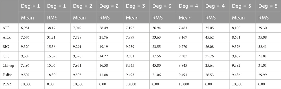
Table 1. Polynomial degree estimates in additive Gaussian noise averaged over all five noise standard deviations.

Table 2

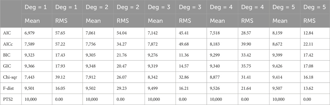
Table 2. Polynomial degree estimates in additive Uniform noise averaged over all five noise standard deviations.

Table 3

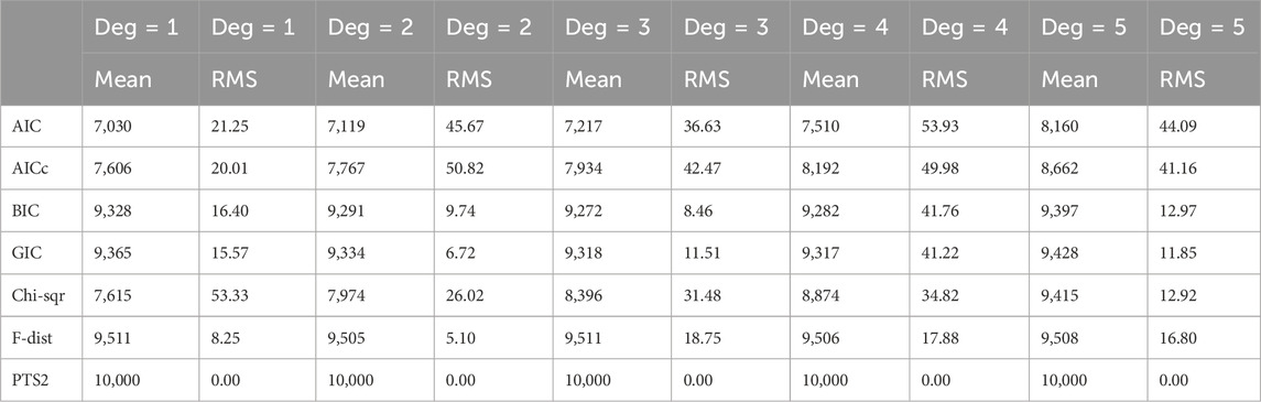
Table 3. Polynomial degree estimates in additive Exponential noise averaged over all five noise standard deviations.

For each of the methods, Figure 1 visualises numbers of correct polynomial degree estimates averaged over all five noise standard deviations in Exponential noise versus each of the polynomial degrees. AIC, AICc, BIC, GIC, Chi-square, F-distribution, and PTS2 results are depicted in ‘up triangle’, ‘down triangle’, ‘plus’, ‘square’, ‘diamond’, ‘star’, and ‘open circle’ respectively. The black solid line represents the ideal values. One can observe that AIC performs the worst, while PTS2 is perfect. It is interesting to note that Tables 1–3 are very similar. The performances of all the seven methods are very similar in three different types of noise. So, we have further averaged Tables 1–3. These combined results from summarizing 15 Tables are displayed in Figure 2. It is clear that Figures 1, 2 are very similar. Below are some observations:

1) AIC performs the worst and PTS2 is perfect.

2) BIC and GIC perform extremely similarly.

3) PTS2 performs better than F-distribution, which performs better than BIC and GIC, which perform better than Chi-square, which performs better than AICc, which performs better than AIC.

4) AIC, AICc, and Chi-square get more accurate as the degree of a polynomial increases.

5) For degree 1, the performance of Chi-square is similar to those of AICc and better than AIC. Notably, the performance of Chi-square gets more accurate more quickly as the degree of a polynomial increases. For example, in the case of degree 5, the performance of Chi-square is similar to those of BIC and GIC, and significantly better than those of AIC and AICc.

6) Performances of PTS2 or F-distribution or BIC and GIC are more stable as the degree of the polynomial increases.

Figure 1

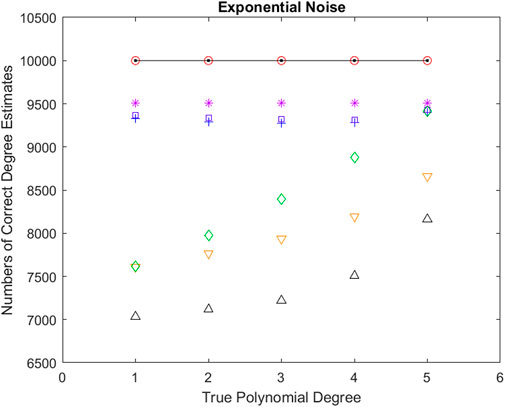
Figure 1. Numbers of correct polynomial degree estimations averaged over all five noise standard deviations in Exponential noise versus each of the polynomial degrees. AIC, AICc, BIC, GIC, Chi-square, F-distribution, and PTS2 results are depicted in “up triangle”, “down triangle”, “plus”, “square”, “diamond”, “star”, and “open circle” respectively. The black solid line represents the ideal values. AIC performs the worst, while PTS2 is perfect.

Figure 2

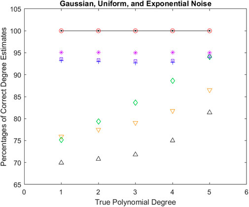
Figure 2. Percentages of correct polynomial degree estimations averaged over all five noise standard deviations as well as averaged over all three noise types (Gaussian, Uniform, and Exponential noise) versus each of the polynomial degrees. AIC, AICc, BIC, GIC, Chi-square, F-distribution, and PTS2 results are depicted in “up triangle”, “down triangle”, “plus”, “square”, “diamond”, “star”, and “open circle” respectively. The black solid line represents the ideal values. AIC performs the worst, while PTS2 is perfect.

3.3 Noise standard deviation estimation

For each type of noise distribution, we have generated 10,000 realisations for each combination of polynomial degrees (1, 2, 3, 4, and 5) and five different strengths of additive noise (standard deviations of 1, 2, 4, 7, and 10), where each realization has 101 data values. These have been used to estimate the noise standard deviations added to a polynomial using seven model order selection methods (AIC, AICc, GIC, BIC, Chi-square, F-distribution, and PTS2). The PTS2 accurately estimated the polynomial degree every time, but none of the other six methods were anywhere near as accurate and they themselves had different performances. For this study, unlike in Section 3.2, we have helped the other six methods by making available the correct polynomial degree in each case. Of course, this has allowed their results to have been artificially enhanced, but it allows us to compare with much better outcomes. These have been organized in five Tables. Each Table recorded the estimated noise and the standard deviation of the estimated noise from each of the seven methods for each of the five polynomial degrees.

There are five such Tables for each type of additive noise. It should be noted that, within each of these five Tables, seven methods offer very similar results. As an example, this can be observed in Table 4, which presents the results for the $\sigma$ values of 1 and 10. Since, all the ideal values in each of these five Tables are different (1 or 2 or 4 or 7 or 10) it does not make sense to aggregate them directly. Yet, a close study of Table 4 indicates that, if one were to normalise the individual five Tables by the corresponding true value of $\sigma$, all the values from different methods and Tables are similar. Therefore, the numbers in each of these five Tables have been normalized by the corresponding true value of the additive noise, ensuring that all the ideal values of noise in each of these five Tables are the same and it is 1. Finally, to avoid too many Tables and yet to aggregate all the information, we have averaged five normalized Tables into one Table. Table 5, Table 6, and Table 7 represent the summary results on noise estimation in additive Gaussian noise, Uniform noise, and Exponential noise respectively.

Table 4

Table 4. Noise standard deviation estimates of additive Gaussian noise.

Table 5

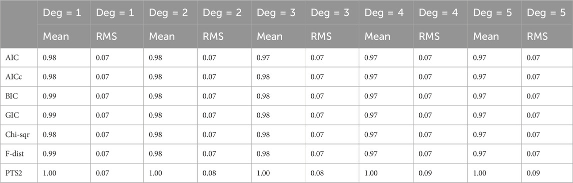
Table 5. Normalised noise standard deviation estimates of additive Gaussian noise averaged over all five noise standard deviations.

Table 6

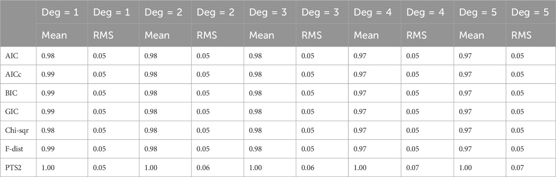
Table 6. Normalised noise standard deviation estimates of additive Uniform noise averaged over all five noise standard deviations.

Table 7

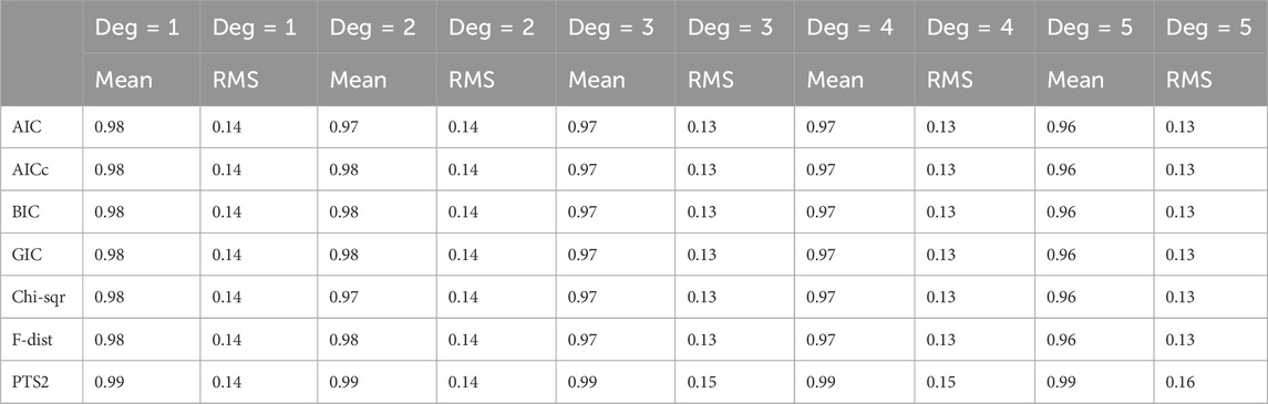
Table 7. Normalised noise standard deviation estimates of additive Exponential noise averaged over all five noise standard deviations.

It should be remembered that for this study, unlike in Section 3.2, we have helped the six methods (AIC. AICc, BIC, GIC, Chi-square, and F-distribution) by making available the correct polynomial degree in each case. Below are some observations:

1) In Table 5, PTS2 is the best and the other six methods are much the same.

2) In both Tables 6 and 7, PTS2 is the best and the other six methods are much the same.

3) It is interesting to note that the normalized mean value estimates of the additive noise in Tables 5–7 are very similar for each method.

4) The RMS (root-mean-square) values of normalized mean noise estimates from all methods for polynomial degrees of 1–5 are different in different types of noise. Typically, they are 0.05 in Uniform noise, 0.07 in Gaussian noise, and 0.13 in Exponential noise.

As the performance of all the seven methods are very similar in three different types of noise, we have further averaged Tables 5–7. Using these combined results from summarizing 15 Tables, Figure 3 visualises the mean value of the normalized standard deviation of the additive noise averaged over all five noise standard deviations and averaged over all three noise types (Gaussian, Uniform, and Exponential noise). F-distribution (as a representative of AIC, AICc, BIC, GIC, Chi-square, and F-distribution) and PTS2 results are represented by ‘star’ and ‘open circle’ respectively. The black solid line represents the ideal values. One can observe that both PTS2 and F-distribution performance are very good. PTS2 performances are perfect some of the times and are near perfect other times, but the ones from F-distribution and the other five methods are never perfect. It is clear that the PTS2 performances are better than the performances from the other six methods.

Figure 3

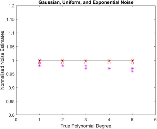
Figure 3. Mean values of the normalized standard deviation of the additive noise averaged over all five noise standard deviations and averaged over all three noise types (Gaussian, Uniform, and Exponential noise) versus each of the polynomial degrees. F-distribution (as a representative of AIC, AICc, BIC, GIC, Chi-square, and F-distribution) and PTS2 results are represented by ‘star’ and ‘open circle’ respectively. The black solid line represents the ideal values. Although both PTS2 and F-distribution performance are very good, PTS2 performances are better than the performances of the other six methods.

3.4 Polynomial coefficient corresponding to the highest degree estimation

For each type of noise distribution, we have generated 10,000 realisations for each combination of polynomial degrees (1, 2, 3, 4, and 5) and five different strengths of additive noise (standard deviations of 1, 2, 4, 7, and 10), where each realization has 101 data values. These have been used to estimate the highest degree coefficient of polynomial using seven model order selection methods (AIC, AICc, GIC, BIC, Chi-square, F-distribution, and PTS2). For this study, unlike in Section 3.2, the true value of the polynomial degree has been used for AIC, AICc, BIC, GIC, Chi-square, and F-distribution to obtain a more accurate estimate of the value of the highest degree coefficient. While this has allowed their results to have been artificially enhanced, it has allowed us to compare with better outcomes. These have been organized in five Tables. Each Table recorded the estimated value of the polynomial coefficient corresponding to the highest degree and its standard deviation from each of the seven methods for each of the five polynomial degrees. There are five such Tables for one type of additive noise. Remember that all the ideal values in each of these five Tables are not the same (2 for degree 1 and 4 for degree 2 and 8 for degree 3 and 16 for degree 4 and 32 for degree 5). Yet, for each degree the ideal value is the same in each of these five Tables. Therefore, the numbers in each of these five Tables have been averaged degree by degree, for each of the three different noise types. Table 8, Table 9, and Table 10 represent the summary results on estimated value of the polynomial coefficient corresponding to the highest degree and its standard deviation in Gaussian noise, Uniform noise, and Exponential noise respectively.

Table 8

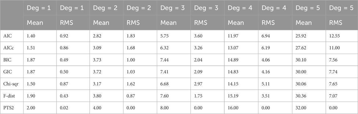
Table 8. Estimates of the polynomial coefficient corresponding to the highest degree in additive Gaussian noise averaged over all five noise standard deviations.

Table 9

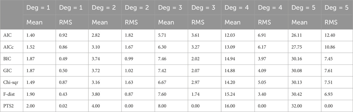
Table 9. Estimates of the polynomial coefficient corresponding to the highest degree in additive Uniform noise averaged over all five noise standard deviations.

Table 10

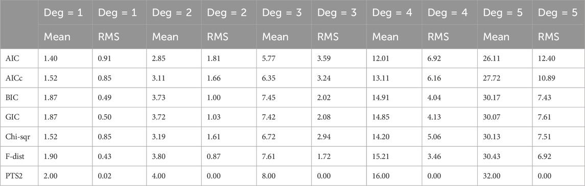
Table 10. Estimates of the polynomial coefficient corresponding to the highest degree in additive Exponential noise averaged over all five noise standard deviations.

It should be remembered that for this study, unlike in Section 3.2, we have helped the six methods (AIC. AICc, BIC, GIC, Chi-square, and F-distribution) with the knowledge of the correct polynomial degree in each case. Below are some observations:

1) Considering the mean or the standard deviation estimates of the highest degree coefficient of polynomial estimates, AIC performs the worst and PTS2 is the best.

2) BIC and GIC perform extremely similarly. F-distribution performs slightly better than BIC and GIC, as its mean is always slightly nearer to the true value and its standard deviation is always smaller.

3) PTS2 outperforms F-distribution, which performs better than BIC and GIC, which perform better than AICc, which performs better than AIC.

4) For degree 1, the performance of Chi-square is similar to those of AIC and AICc. But the performance of Chi-square gets more accurate as the degree of a polynomial increases. For example, in the case of degree 5, the performance of Chi-square is similar to those of BIC and GIC, and significantly better than those of AIC and AICc.

5) Mean estimates of PTS2 are ideal with extremely small standard deviations.

As the performance of all the seven methods are very similar in three different types of noise, we have further averaged Tables 8–10. Using these combined results from summarizing 15 Tables, Figure 4 presents the mean of the polynomial coefficient corresponding to the highest degree estimates from all seven methods averaged over all five noise standard deviations and averaged over all three noise types (Gaussian, Uniform, and Exponential noise) versus each of the polynomial degrees. AIC, AICc, BIC, GIC, Chi-square, F-distribution, and PTS2 results are depicted in ‘up triangle’, ‘down triangle’, ‘plus’, ‘square’, ‘diamond’, ‘star’, and “open circle” respectively. The black solid line indicates the ideal values. One can observe that PTS2 performances are perfect and are very much better than the remaining six methods.

Figure 4

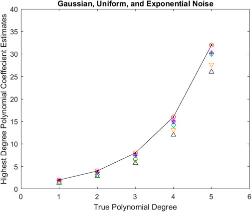
Figure 4. Mean values of estimates of the polynomial coefficient corresponding to the highest degree from all seven methods averaged over all five noise standard deviations and averaged over all three additive noise types (Gaussian, Uniform, and Exponential noise) versus each of the polynomial degrees. AIC, AICc, BIC, GIC, Chi-square, F-distribution, and PTS2 results are depicted in “up triangle”, “down triangle”, “plus”, “square”, “diamond”, “star”, and “open circle” respectively. The black solid line indicates the ideal values. One can observe that PTS2 performances are perfect and are very much better than the remaining six methods.

Figure 5 displays the standard deviation of the polynomial coefficient corresponding to the highest degree estimates from all seven methods averaged over all five noise standard deviations and averaged over all three noise types (Gaussian, Uniform, and Exponential noise) versus each of the polynomial degrees. AIC, AICc, BIC, GIC, Chi-square, F-distribution, and PTS2 results are depicted in “up triangle”, “down triangle”, “plus”, “square”, “diamond”, “star”, and “open circle” respectively. The black solid line represents the ideal values. One can observe that PTS2 performances are extremely accurate and are much better than the remaining six methods. AIC performs the worst.

Figure 5

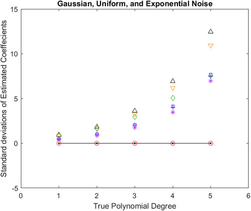
Figure 5. Standard deviations of estimates of the polynomial coefficient corresponding to the highest degree from all seven methods averaged over all five noise standard deviations and averaged over all three additive noise types (Gaussian, Uniform, and Exponential noise) versus each of the polynomial degrees. AIC, AICc, BIC, GIC, Chi-square, F-distribution, and PTS2 results are depicted in “up triangle”, “down triangle“, “plus”, “square”, “diamond”, “star”, and “open circle” respectively. The black solid line represents the ideal values. One can observe that PTS2 performances are extremely accurate and are very much better than the remaining six methods. AIC performs the worst.

4 Conclusion

This study has explored time-series representations of polynomials. The major contributions of this paper lie in the original research offering novel theoretical and experimental results. The theoretical results have included 1) an alternative proof of the qth order AR time-series representation, with a constant, of a polynomial of degree q, 2) an alternative proof of the (q + 1)-th order AR time-series representation, without a constant, of a polynomial of degree q, as well as 3) generalized equations (valid for a polynomial of an arbitrary degree) for reduced variance estimation of the polynomial coefficient corresponding to the highest degree. The reported experimental investigations are the most comprehensive so far, in that they have used well over 35 times more realisations than before, have used a wider variety of noisy data using zero-mean Gaussian, Uniform, and Exponential noise, and have used a larger range of polynomial degrees as well as of noise standard deviations than before. Experimental results on estimations of the degree of a polynomial, of the additive noise standard deviation, and of the polynomial coefficient corresponding to the highest degree using seven methods (AIC, AICc, BIC, GIC, Chi-square, F-distribution, and PTS2) have been presented.

In the estimations of the degree of a polynomial, AIC performs the worst while PTS2 is perfect. PTS2 performs better than F-distribution, which performs better than BIC and GIC, which perform better than AICc, which performs better than AIC. For degree 1, the performance of Chi-square is similar to those of AICc and better than AIC. Notably, the performance of Chi-square gets more accurate more quickly as the degree of a polynomial increases. For example, in the case of degree 5, the performance of Chi-square is similar to those of BIC and GIC, and significantly better than those of AIC and AICc.

In estimations of additive noise standard deviations, the performance of PTS2 is the best and the other six methods (with the exact knowledge of the degree) are much the same. The RMS values of normalized mean noise estimates from all methods for polynomial degrees of 1–5 are different in different types of noise. Typically, they are 0.05 in Uniform noise, 0.07 in Gaussian noise, and 0.13 in Exponential noise, In estimations of the polynomial coefficient corresponding to the highest degree, AIC performs the worst and PTS2 is the best. PTS2 outperforms F-distribution, which performs better than BIC and GIC, which perform better than AICc, which performs better than AIC. For degree 1, the performance of Chi-square is similar to those of AIC and AICc. Notably, the performance of Chi-square gets more accurate more quickly as the degree of a polynomial increases. For example, in the case of degree 5, the performance of Chi-square is similar to those of BIC and GIC, and significantly better than those of AIC and AICc. Mean estimates of PTS2 are ideal with extremely small standard deviations.

The paradigm and techniques discussed here can be useful in many diverse practical applications, e.g. (Fernandez-Jimenez et al., 2012; Monin et al., 2014; Moskalev et al., 2011; Nandi et al., 2020c; Sivaraman et al., 2024; Zhang et al., 2025), as well as many others.

Data availability statement

The raw data supporting the conclusions of this article will be made available by the authors, without undue reservation.

Author contributions

AN: Conceptualization, Data curation, Formal Analysis, Funding acquisition, Investigation, Methodology, Project administration, Resources, Software, Supervision, Validation, Visualization, Writing – original draft, Writing – review and editing.

Funding

The author(s) declare that no financial support was received for the research and/or publication of this article.

Acknowledgments

The author acknowledges Chao Liu for formatting the manuscript to the journal style file.

Conflict of interest

The author declares that the research was conducted in the absence of any commercial or financial relationships that could be construed as a potential conflict of interest.

Generative AI statement

The author(s) declare that no Generative AI was used in the creation of this manuscript.

Publisher’s note

All claims expressed in this article are solely those of the authors and do not necessarily represent those of their affiliated organizations, or those of the publisher, the editors and the reviewers. Any product that may be evaluated in this article, or claim that may be made by its manufacturer, is not guaranteed or endorsed by the publisher.

References

Abramowitz, M., and Stegun, I. A. (1972). Handbook of mathematical functions: with formulas, graphs, and mathematical Tables. New York: Dover Publications.

Google Scholar

Akaike, H. (1974). A new look at the statistical model identification. IEEE Trans. Autom. Contr 19, 716–723. doi:10.1109/tac.1974.1100705

CrossRef Full Text | Google Scholar

Akaike, H. (1978). On the likelihood of a time series model. Statistician 27, 217–235. doi:10.2307/2988185

CrossRef Full Text | Google Scholar

Bhansali, R. J., and Downham, D. Y. (1977). Some properties of the order of an autoregressive model selected by a generalization of akaike’s EPF criterion. Biometrika 64, 547–551. doi:10.2307/2345331

CrossRef Full Text | Google Scholar

Burnham, K. P., and Anderson, D. R. (2002). Model selection and multimodel inference. New York: Springer.

Google Scholar

Burnham, K. P., and Anderson, D. R. (2004). Multimodel inference: understanding AIC and BIC in model selection. Sociol. Methods Res. 33, 261–304. doi:10.1177/0049124104268644

CrossRef Full Text | Google Scholar

Cavanaugh, J. E. (1997). Unifying the derivations for the Akaike and corrected Akaike information criteria. Stat. Probab. Lett. 33, 201–208. doi:10.1016/S0167-7152(96)00128-9

CrossRef Full Text | Google Scholar

Claeskens, G., and Hjort, N. L. (2008). Model selection and model averaging. Cambridge University Press.

Google Scholar

Fernandez-Jimenez, N., Plaza-Izurieta, L., Lopez-Euba, T., Jauregi-Miguel, A., and Ramon Bilbao, J. (2012). Cubic regression-based degree of correction predicts the performance of whole bisulfitome amplified DNA methylation analysis. Epigenetics 7, 1349–1354. doi:10.4161/epi.22846

PubMed Abstract | CrossRef Full Text | Google Scholar

Kashyap, R. L. (1982). Optimal choice of AR and MA parts in autoregressive moving average models. IEEE Trans. Pattern Anal. Mach. Intell. PAMI-4, 99–104. doi:10.1109/TPAMI.1982.4767213

PubMed Abstract | CrossRef Full Text | Google Scholar

Konishi, S., and Kitagawa, G. (2008). Information criteria and statistical modeling. 1st Edn. Incorporated: Springer Publishing Company.

Google Scholar

Linhart, H., and Zucchini, W. (1986). Model selection. Wiley.

Google Scholar

Monin, P., Bosmans, H., Verdun, F. R., and Marshall, N. W. (2014). Comparison of the polynomial model against explicit measurements of noise components for different mammography systems. Phys. Med. Biol. 59, 5741–5761. doi:10.1088/0031-9155/59/19/5741

CrossRef Full Text | Google Scholar

Moskalev, E. A., Zavgorodnij, M. G., Majorova, S. P., Vorobjev, I. A., Jandaghi, P., Bure, I. V., et al. (2011). Correction of PCR-bias in quantitative DNA methylation studies by means of cubic polynomial regression. Nucleic Acid. Res. 39, e77. doi:10.1093/nar/gkr213

PubMed Abstract | CrossRef Full Text | Google Scholar

Nandi, A. K. (2020a). Data modeling with polynomial representations and autoregressive time-series representations, and their connections. IEEE Access 8, 110412–110424. doi:10.1109/ACCESS.2020.3000860

PubMed Abstract | CrossRef Full Text | Google Scholar

Nandi, A. K. (2020b). Model order selection from noisy polynomial data without using any polynomial coefficients. IEEE Access 8, 130417–130430. doi:10.1109/ACCESS.2020.3008527

CrossRef Full Text | Google Scholar

Nandi, A. K. (2021). Degree and noise power estimation from noisy polynomial data via AR modelling. Digit. Signal Process 114, 103071. doi:10.1016/j.dsp.2021.103071

CrossRef Full Text | Google Scholar

Nandi, A. K., Roberts, D. J., and Nandi, A. K. (2020c). Improved long-term time-series predictions of total blood use data from England. Transfusion 60, 2307–2318. doi:10.1111/trf.15966

PubMed Abstract | CrossRef Full Text | Google Scholar

Schwarz, G. (1978). Estimating the dimension of a model. Ann. Statistics 6, 461–464. doi:10.1214/aos/1176344136

CrossRef Full Text | Google Scholar

Sivaraman, D., Ongwattanakul, S., Pillai, B. M., and Suthakorn, J. (2024). Adaptive polynomial Kalman filter for nonlinear state estimation in modified AR time series with fixed coefficients. IET Control Theory and Appl. 18, 1806–1824. doi:10.1049/cth2.12727

CrossRef Full Text | Google Scholar

Stoica, P., and Selen, Y. (2004). Model-order selection: a review of information criterion rules. IEEE Signal Process Mag. 21, 36–47. doi:10.1109/MSP.2004.1311138

CrossRef Full Text | Google Scholar

Sugiura, N. (1978). Further analysis of the data by Akaike’s information criterion and the finite corrections. Commun. Stat. Theory Methods 7, 13–26. doi:10.1080/03610927808827599

CrossRef Full Text | Google Scholar

Vrieze, S. I. (2012). Model selection and psychological theory: a discussion of the differences between the Akaike information criterion (AIC) and the Bayesian information criterion (BIC). Psychol. Methods 17, 228–243. doi:10.1037/a0027127

PubMed Abstract | CrossRef Full Text | Google Scholar

Wikipedia (2025a). Chi-squared test. Available online at: https://en.wikipedia.org/wiki/Chi-squared_test.

Google Scholar

Wikipedia (2025b). F-test. Available online at: https://en.wikipedia.org/wiki/F-test#Regression_problems.

Google Scholar

Yang, Y. (2005). Can the strengths of AIC and BIC Be shared? A conflict between model identification and regression estimation. Biometrika 92, 937–950. doi:10.1093/biomet/92.4.937

CrossRef Full Text | Google Scholar

You, P., Ding, Z., Qian, L., Li, M., Zhou, X., Liu, W., et al. (2019). A motion parameter estimation method for radar maneuvering target in Gaussian clutter. IEEE Trans. Signal Process. 67, 5433–5446. doi:10.1109/TSP.2019.2939082

CrossRef Full Text | Google Scholar

Zhang, J., Zeng, C., Tao, H., Zhang, Y., Zhao, S., and Wu, Q. (2025). A broken-track association method for robust multi-target tracking adopting multi-view Doppler measurement information. Signal Process. 230, 109815. doi:10.1016/j.sigpro.2024.109815

CrossRef Full Text | Google Scholar