Deep learning-based GNSS composite jamming detection and recognition technology

As the interference environment of Global Navigation Satellite Systems (GNSS) becomes increasingly complex and diverse, real-time and precise interference detection and identification technologies are crucial for enhancing the anti-interference capabilities of receivers. However, most existing interference detection and identification methods focus on single interference types, with limited research on composite interference and a lack of quantitative conclusions. Therefore, this study investigates composite interference detection and identification techniques using deep learning methods, improving the system’s capability to detect and identify composite interference. This paper first constructs single interference model and composite interference model, proposes three signal preprocessing methods, and generates corresponding image datasets. Subsequently, the interference detection and identification performance under different signal preprocessing methods is analyzed using the ResNet-18 deep learning neural network. The optimal signal preprocessing method is identified, and quantitative conclusions are obtained. Finally, a lightweight network, LcxNet-Fusion, is designed, which significantly reduces the number of network parameters and forward processing time while maintaining an acceptable level of accuracy reduction. Results show that among the time-frequency 2D diagrams, power spectral diagrams, and histograms generated by signal preprocessing, the time-frequency diagram yields the best detection and identification performance. When the detection rate reaches 90%, the jamming-to-noise ratio (JNR) sensitivity of the time-frequency diagram is −20 dB; when the identification rate reaches 90%, the JNR sensitivity of the time-frequency diagram is −13 dB. On the Tesla V100 GPU, the LcxNet-Fusion network has 24.32 MB parameters, an 43% reduction compared to the ResNet-18 network, with a forward processing time of 1.25 s, reducing by 15%. This work holds promising prospects in the field of interference detection and identification for GNSS systems under complex electromagnetic environments.

1 Introduction

Global Navigation Satellite Systems (GNSS) are widely utilized in transportation, emergency rescue, financial transactions, precision agriculture, and drone navigation, serving as an indispensable technological backbone for the normal functioning of modern society. However, GNSS signals are inherently weak and susceptible to external interference, including intentional interference and unintentional interference. In recent years, GNSS interference events have occurred frequently, disrupting the normal operation of multiple industries. In recent years, GPS interference incidents have frequently occurred during military operations (Buesnel, 2018; Foundation, 2017). For instance, in 2018, multiple GPS interference events were observed in northern Finland during a NATO military exercise, accompanied by warnings about large-scale GPS signal disruptions (Yleisradio, 2018).

These cases highlight the significant challenges faced by GNSS systems in complex electromagnetic environments and emphasize the importance of promptly identifying and addressing interference. Timely and effective interference detection and identification technologies not only help identify potential interference sources and prevent losses caused by malicious attacks but also mitigate the impact of unintentional interference on critical services. For instance, by monitoring GNSS signals in real time, detecting abnormal fluctuations and sudden signal losses, interference sources can be swiftly localized, and necessary measures can be taken to ensure the reliable operation of navigation and positioning systems. Therefore, with the widespread application of GNSS across various fields, developing and implementing advanced interference detection and identification technologies has become increasingly important. This is not only critical to the efficient functioning of the global economy but also essential for societal safety and stability.

Traditional GNSS interference detection and identification methods primarily rely on signal feature analysis and statistical techniques, typically detecting interference by monitoring variations in signal parameters. For example, Sakorn. C et al. proposed a detection method based on signal power and C/N0 analysis, which identifies interference by monitoring noise levels and signal loss in GNSS receivers (Sakorn and Supnithi, 2021). These traditional methods rely on setting threshold values, where the system triggers interference alarms once the signal parameters exceed predefined thresholds. Zhu. W et al. proposed a spectrum analysis method based on Fourier transform to identify interference in GNSS signals (Zhu et al., 2024), while Jeong. S et al. introduced a CUSUM-based GNSS interference detection method (Jeong et al., 2020). This method first collects GNSS signal data to establish a reference model, then calculates and accumulates the deviations between real-time signals and the reference model. Interference is determined when the cumulative deviation exceeds a predefined threshold. Wang. Y et al. designed an SVM-based detection method that leverages feature extraction and selection techniques to extract frequency-domain and time-domain features from GNSS signals, enabling effective interference classification (Wang et al., 2020). Traditional interference detection methods achieve high accuracy under specific conditions but require manual extraction of interference features with explicit physical meanings. They rely on prior knowledge and fixed models, making it difficult to accurately and promptly identify interference types in complex environments. In contrast, deep learning-based GNSS interference detection and identification methods enable automatic recognition of interference signals through model training, improving both accuracy and robustness. For instance, CNN based classification is widely used in signal classification, and results are comparable even in some instances superior results (Cheikh and Soltani, 2006; Chralampidis et al., 2001; Darzikolaei et al., 2015; Ibrahim et al., 2009), which automatically extracts signal features and identifies various interference types by training on historical receiver data. By training on large-scale historical interference datasets, the model can learn the characteristic patterns of different interference types without requiring predefined thresholds for interference recognition. This approach is particularly suited to complex and dynamically changing interference environments, achieving significantly higher detection accuracy than traditional rule-based methods.

Although deep learning methods have demonstrated significant potential, research indicates that they still face several challenges. Firstly, publicly available GNSS interference datasets include only five types of interference, which severely limit the ability of CNN-based methods to learn more complex signal features. The overlapping of multiple interference types in composite interference scenarios has yet to be addressed. Furthermore, the impact of different signal preprocessing methods on deep learning approaches remains unclear and unquantified. Finally, most CNN-based methods utilize typical networks, such as AlexNet (Krizhevsky et al., 2012), ResNet-18 (He et al., 2016), and VGG-11 (Simonyan and Zisserman, 2015), as classifiers, which consume substantial memory. These networks were originally designed for the ImageNet dataset and are not well-suited for interference identification tasks, leading to suboptimal performance.

2 GNSS single interference and composite interference model

Based on the surveyed literature (Borio et al., 2016; Kraus et al., 2011), this section categorizes single interference into five types: single-frequency continuous wave interference, pulse interference, chirp interference, narrowband noise interference, and matched spectral interference. The following are the models for these single and composite interferences.

2.1 Single-frequency continuous wave interference

Single-frequency continuous wave interference (Continuous Wave Jamming, CW) is a persistent interference signal characterized by a fixed frequency and relatively high power. This type of interference appears as a sinusoidal wave with a constant frequency in the time domain and as a pulse centered at the interference frequency in the frequency domain. Its expression is given as:

$J\left(t\right)=\sqrt{P_J}{e}^{j\left(2\pi f_{J}t+{\theta }_J\right)}(1)$

Where $P_J$ is the interference amplitude, $f_J$ is the interference frequency, and ${\theta }_J$ is the interference phase.

2.2 Chirp interference

Chirp interference refers to an electromagnetic interference signal whose frequency continuously varies over time. It disrupts the normal operation of communication devices by continuously altering the frequency of the interference signal within a specific range. Its expression is as follows:

$J\left(t\right)=\sqrt{P_J}{e}^{j\left(2\pi f_{0}t+\pi \frac{f_{\max }-f_{\min }}{T_{swp}}{t}^2+{\theta }_J\right)}(2)$

where $P_J$ is the interference amplitude, $f_0$ is the starting frequency of the chirp, $f_{\max }-f_{\min }$ is the chirp bandwidth, $T_{swp}$ is the chirp period, and ${\theta }_J$ is the interference phase.

2.3 Pulse interference

Pulse interference features high peak power, short duration, and a wide spectrum, providing greater interference efficiency than continuous waves of equivalent power. When the pulse interference center frequency sweeps across a range overlapping the receiver bandwidth, it interferes with the receiver. Its mathematical expression is:

$s_i\left(t\right)=\left\{\begin{array}{l}1-\frac{\tau }{2}+nT\le t\le \frac{\tau }{2}+nT,n=1,2...\\ 0else\end{array}\right.(3)$

$J\left(t\right)=\sqrt{P_J}{e}^{j\left(2\pi f_{J}t+{\theta }_J\right)}s\left(t\right)(4)$

where $P_J$ is the interference amplitude, $f_J$ is the interference frequency, ${\theta }_J$ is the interference phase, $\tau$ is the pulse width, and $T$ is the pulse repetition period.

2.4 Narrow band interference

Narrow Band Gaussian interference (NB) refers to Gaussian noise with a band-width of 1%–10% of the actual bandwidth of the satellite signal. Its expression is:

$J\left(t\right)=\sqrt{P_J}{e}^{j\left(2\pi f_{J}t+{\theta }_J\right)}\otimes h\left(t\right)(5)$

$\begin{array}{l}H\left(j2\pi f\right)=\left\{\begin{array}{l}1,\left|f\right|\le W_I\\ 0,\text{otherwise}\end{array}\right.\end{array}(6)$

where $P_J$ is the interference amplitude, $f_J$ is the interference frequency, ${\theta }_J$ is the interference phase, $h\left(t\right)$ is a low-pass filter that controls the bandwidth of Narrow Band interference.

2.5 Matched spectral interference

Matched spectral interference is a type of interference signal that matches the spectral characteristics of the target signal. Unlike traditional broadband or narrow band interference, matched spectral interference is highly customized, making it nearly indistinguishable from the target signal. This significantly increases the decoding difficulty for the receiver. Its expression is given as follows:

$J\left(t\right)=P_J{p}_N\left(t\right)d\left(t\right)e^{j\left(2\pi f_{J}t+{\theta }_J\right)}(7)$

here $P_J$ is the interference amplitude, $f_J$ is the interference frequency, and ${\theta }_J$ is the interference phase, $P_N\left(t\right)$ is the p-code, $d\left(t\right)$ is the navigation messages.

2.6 Composite interference

In complex electromagnetic environments, GNSS receivers often face interference signals from various sources. These types of interference not only take diverse forms but are also growing increasingly complex. Composite interference, as an efficient form of interference, combines different types of interference signals to produce more pronounced effects, severely disrupting the normal operation of GNSS systems. Composite interference is generally defined in the following categories.

2.6.1 Composite interference of suppression and deception

Composite interference of suppression and deception refers to the combination of the characteristics of both suppression and deception interference to achieve more sophisticated interference effects. The process typically involves first using suppression interference to disable the receiver’s ability to acquire real satellite signals. Subsequently, deceptive signals are used to transmit false satellite signals, leading to positioning misguidance that not only prevents the victim system from recognizing genuine signals but also guides it to an erroneous state.

2.6.2 Composite interference with multiple modulation methods

Composite interference with multiple modulation methods refers to the combination of various modulation techniques during the interference process to enhance the interference effectiveness and the complexity of anti-interference measures. For example, narrowband interference can be modulated within the continuous wave interference frequency band, creating new interference components within the receiver and increasing the difficulty of interference detection, identification, and anti-jamming efforts.

2.6.3 Composite interference with multiple interferences

Composite interference with multiple interferences refers to the superposition of multiple types of interference signals within the same frequency spectrum, forming a complex interference field. The superimposed interference signals may originate from devices with different frequency bands and power levels. Due to differences in the spectral and time-domain characteristics of these signals, the resulting interference effects are highly complex, making it difficult for the receiver to distinguish between interference sources, which severely degrades GNSS positioning performance.

Due to the widespread application of wireless communication, radar, broadcasting, remote sensing, and other systems, multiple signal sources are typically present in urban environments, industrial zones, and military areas. These signal sources, with varying frequency ranges, power levels, and modulation methods, are highly prone to forming composite interference with multiple interferences. Therefore, this paper focuses on investigating the scenario of composite interference with multiple interferences. The schematic diagram and mathematical expression of the composite interference are shown as Figure 1 and Equation 8.

$J\left(t\right)={\displaystyle \sum ^N}{J}_N\left(t\right)=J_1\left(t\right)+J_2\left(t\right)+\cdots J_N\left(t\right)(8)$

Figure 1

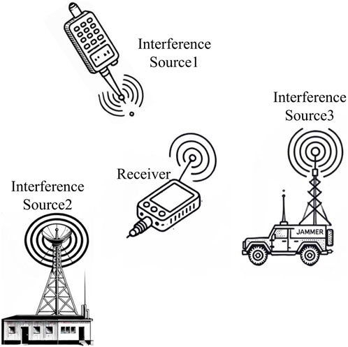
Figure 1. Composite interference.

Where $N$ represents the number of individual interference types. For example, when $N=3$ composite interference can be expressed as:

$\begin{array}{l}J\left(t\right)=J_1\left(t\right)+J_2\left(t\right)+J_3\left(t\right)\\ =J_{\text{PULSE}}\left(t\right)+J_{\text{CW}}\left(t\right)+J_{\text{NB}}\left(t\right)\\ =\sqrt{P_{J_1}}\exp \left(j\left(2\pi f_{J_1}t+{\theta }_{J_1}\right)\right)s\left(t\right)+\sqrt{P_{J_2}}\exp \left(j\left(2\pi f_{J_2}t+{\theta }_{J_2}\right)\right)\\ +\sqrt{P_{J_3}}\exp \left(j\left(2\pi f_{J_3}t+{\theta }_{J_3}\right)\right)\otimes h\left(t\right)\end{array}(9)$

3 Signal preprocessing method

Signal preprocessing is a critical step in signal analysis, aiming to transform raw-data into datasets suitable for analysis, modeling, or deep learning. Directly inputting raw signal data into neural networks without preprocessing increases the burden of feature extraction, necessitates complex and powerful network models, and imposes high demands on data volume and computational resources. Signal preprocessing methods make hidden features explicit, reduce the complexity of raw signals, facilitate more efficient feature learning by models, lower the difficulty of model training, and shorten training time. The field of signal processing typically explores signal characteristics from multiple dimensions, such as time-domain, frequency-domain, and time-frequency domain features. Selecting appropriate signal preprocessing methods is crucial, depending on specific application scenarios and requirements. This study employs three preprocessing methods to evaluate their impact on interference detection and recognition.

(1) Time-domain histogram distribution (Huang et al., 2024): used to extract statistical features of signals in the time domain. Many interferences exhibit randomness or deviation from normal signals in their time-domain distribution, which can be effectively distinguished through histogram analysis. Moreover, time-domain histogram analysis is computationally simple, easy to implement, and has low complexity, making it highly suitable for large-scale real-time processing.

(2) Power spectral transformation (Macii et al., 2001): used to represent the energy distribution of signals in the frequency domain, revealing periodic or frequency component characteristics. Many interferences exhibit specific frequency characteristics in the frequency domain, which can be effectively detected and identified through power spectral analysis. Additionally, power spectral analysis has strong noise resistance, enabling clearer extraction of signal features in noisy environments.

(3) Time-frequency transformation (Wei and Mo, 2025): In non-stationary scenarios, the frequency components of a signal may vary over time, making it difficult for time-domain or frequency-domain analysis alone to comprehensively characterize the signal features. Time-frequency transformation reveals time-varying frequency characteristics on a two-dimensional time-frequency plane, enabling the description of transient characteristics. In many applications, interference may be transient or time-varying, making time-frequency transformation an effective analytical tool. Time-frequency transformation captures spectral information varying with time and extracts time-frequency image features. These two-dimensional features are well suited for integration with deep learning techniques for pattern recognition and classification. This method effectively handles non-stationary signals, which is particularly important for analyzing such signals.

3.1 Time-domain histogram distribution

The time domain histogram characterizes the amplitude distribution of a signal in the time domain. The horizontal axis depicts the real part of the signal’s amplitude, while the vertical axis indicates its occurrence count. The formula for computing the time domain histogram is as follows. First, identify the amplitude range of the signal $\left[n\right]$ , defined by its maximum $x_{\max }$ and minimum $x_{\min }$ . The amplitude range $\left[x_{\max },x_{\min }\right]$ is then divided into equal width intervals $B$.

$\Delta x=\frac{x_{\max }-x_{\min }}{B}(10)$

For each interval, the number of signal samples falling within that interval is counted. Assuming the range of the bth interval is $\left[x_b,x_{b+1}\right]$ , the corresponding statistical quantity $N_b$ is calculated as:

$N_b={\displaystyle \sum _{n=1}^N}\mathrm{I}\mathrm{I}\left(x_b<x\left[n\right]<x_{b+1}\right)(11)$

Where $\mathrm{I}\mathrm{I}$ represents the indicator function, which takes the value of 1 when the condition is true, otherwise 0.

Taking CHIRP interference as an example, its time-domain histogram is shown in Figure 2.

Figure 2

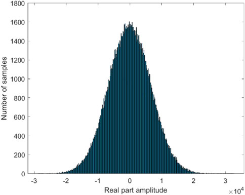
Figure 2. Histogram legend of CHIRP.

The x-axis represents the real part amplitude, while the y-axis represents the number of statistical samples.

The absence of x-y axis information is intentional, as image datasets for deep learning training should retain only the most useful image features while removing redundant elements (such as axes and scale markers). This helps the convolutional neural network (CNN) focus on learning distinguishing features between different labels, thereby improving training performance. Based on the interference model described in Section 2, a subset of interference histogram datasets was generated at a JNR of 0 dB, as shown in Figure 3.

Figure 3

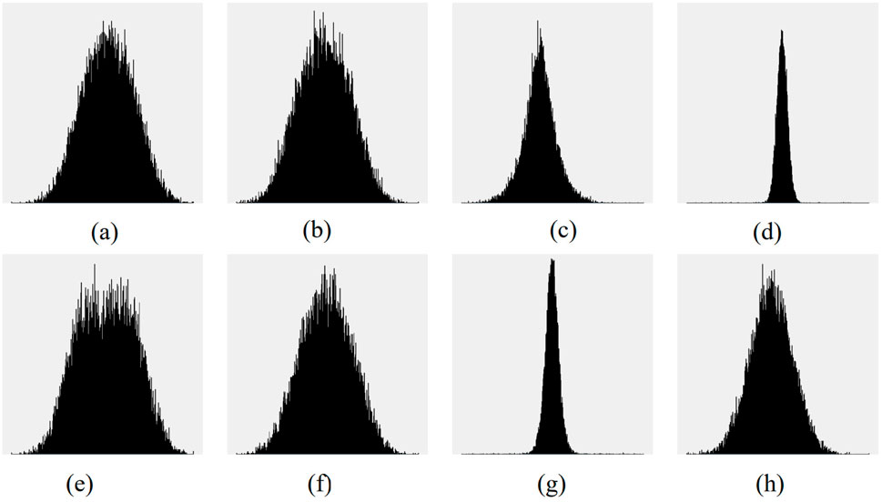
Figure 3. Histogram legend of interference at 0 dB. (a) CW. (b) CHIRP. (c) NB. (d) PULSE. (e) MATCH. (f) MATCH_CHIRP. (g) NB_PULSE. (h) noJam.

It can be intuitively observed that different types of interference exhibit distinct characteristics in the time-domain histogram distribution. These features can be effectively used as inputs to neural networks for interference recognition. However, the characteristics of CW and CHIRP interference are similar in the time-domain histogram, making it likely to confuse their recognition results during interference identification. When the JNR increases to 9 dB, the histograms of the aforementioned types of interference are illustrated, for example, in Figure 4.

Figure 4

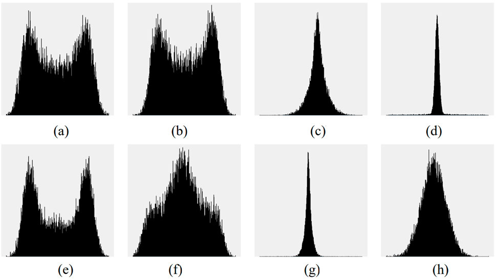
Figure 4. Histogram legend of interference at 9 dB. (a) CW. (b) CHIRP. (c) NB. (d) PULSE. (e) MATCH. (f) MATCH_CHIRP. (g) NB_PULSE. (h) noJam.

It can be observed that as the JNR increases, all types of interference exhibit more distinct characteristics. However, the images of CW and CHIRP interference remain similar, indicating that their recognition results are likely to remain confused in the histogram recognition process, even as JNR increases. In contrast, the recognition rates of other types of interference improve significantly as the JNR increases.

3.2 Power spectral transformation

The power spectral density (PSD) characterizes the energy distribution of a signal within the frequency domain. The horizontal axis indicates the frequency, while the vertical axis denotes the amplitude or power associated with the frequency. For discrete signals $\left[n\right]$ , the power spectrum is derived using the discrete Fourier transform (DFT). The DFT of the signal is defined as $\left[k\right]$ :

$X\left[k\right]={\displaystyle \sum _{n=0}^{N-1}}x\left[n\right]e^{-j2\pi kn/N}(12)$

The PSD is:

$S\left[k\right]=\frac{1}{N}{\left|X\left[k\right]\right|}^2(13)$

Taking CHIRP interference as an example, its PSD is shown in Figure 5.

Figure 5

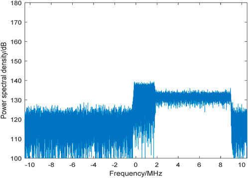
Figure 5. PSD legend of CHIRP.

Where $S\left[k\right]$ represents the power spectral density of the signal at the $k$ frequency, and $N$ represents the length of the DFT. The x-axis indicates the frequency, while the y-axis denotes the amplitude or power associated with the frequency. The PSD plots of some interference types at a JNR of 0 dB are shown in Figure 6.

Figure 6

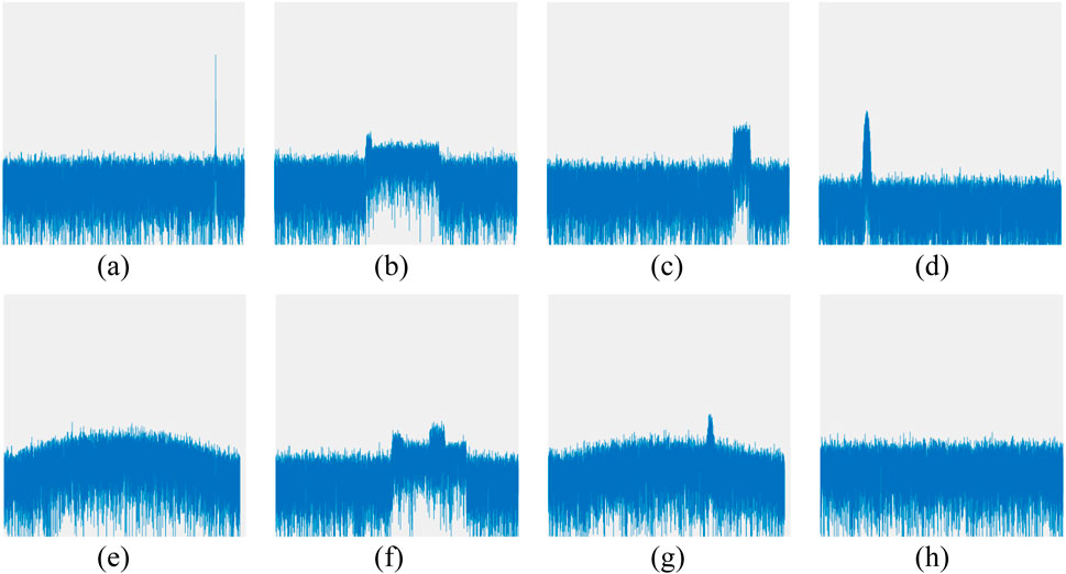
Figure 6. PSD legend of interference at 0 dB. (a) CW. (b) CHIRP. (c) NB. (d) PULSE. (e) MATCH. (f) NB_CHIRP. (g) MATCH_PULSE. (h) noJam.

It can be observed that the distinguishing features of different types of interference are more pronounced in the power spectrum and show significant differences compared to the characteristics in the absence of interference. This suggests that using the PSD for interference detection and recognition yields better results compared to histograms.

3.3 Time-frequency transformation

The time-frequency 2D diagram is used to represent the relationship between time and frequency. Common time-frequency transformation methods include the Short-Time Fourier Transform (STFT), Continuous Wavelet Transform (CWT), Wigner-Ville Distribution (WVD), and Hilbert-Huang Transform (HHT). The advantages and disadvantages of various time-frequency transformation methods are summarized in Table 1.

Table 1

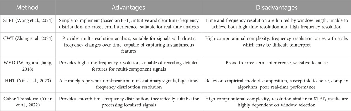
Table 1. Advantages and disadvantages of various time-frequency transformation methods.

Although STFT has certain limitations in terms of resolution, it provides good computational efficiency and intuitiveness in practical applications. It is a widely used general purpose time-frequency analysis tool in engineering, medicine, and science. STFT is often the preferred method for scenarios requiring fast, efficient, and reliable signal analysis. Based on these criteria, this paper adopts the STFT method for analysis. The basic principle involves segmenting the signal and performing Fourier transforms on each segment to observe how the signal frequency changes over time. The main formula of STFT is as follows:

$X\left[t,f\right]={\displaystyle \sum _{n=-\infty }^{\infty }}x\left[n\right]\omega \left[n-t\right]e^{-j2\pi fn/N}(14)$

$X\left[t,f\right]$ is the output of STFT, representing complex values of time and frequency. $\omega \left[n\right]$ represents the window function.

Taking CHIRP interference as an example, its Spectrogram is shown in Figure 7.

Figure 7

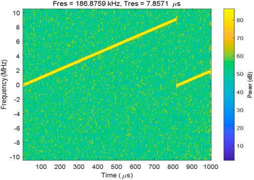
Figure 7. Spectrogram legend of CHIRP.

The x-axis indicates the time, while the y-axis represents the frequency. The time-frequency diagrams of some interference types at a JNR of 0 dB are shown, for example, in Figure 8.

Figure 8

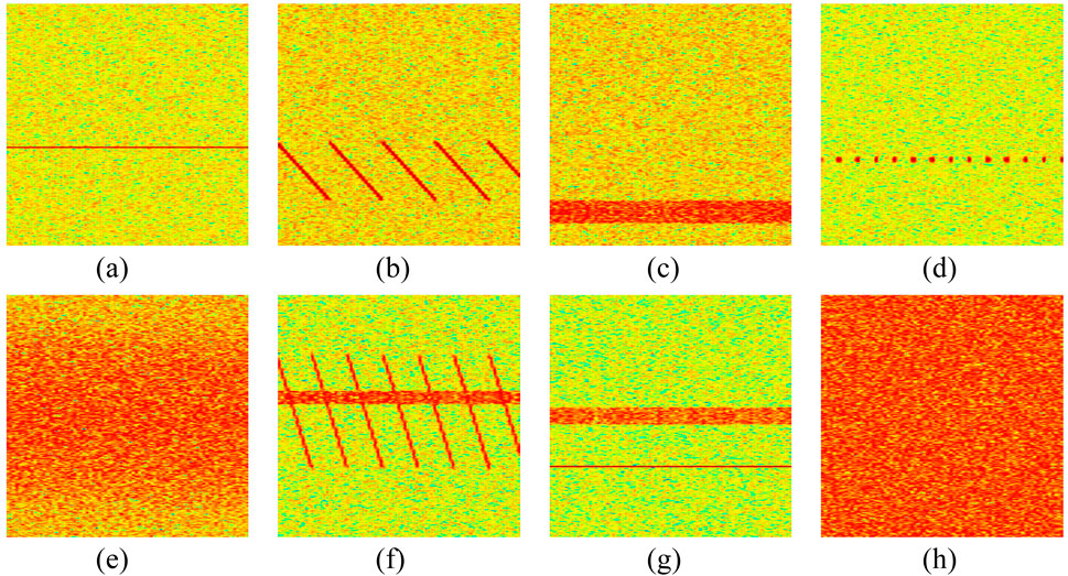
Figure 8. Time-frequency diagrams legend of interference at 0 dB. (a) CW. (b) CHIRP. (c) NB. (d) PULSE. (e) MATCH. (f) NB_CHIRP. (g) NB_CW. (h) noJam.

It can be observed that interference exhibits distinct characteristics in time-frequency diagrams, and the time-frequency diagram of composite interference is a superposition of the corresponding single interference diagrams. This suggests that time-frequency diagram-based detection and recognition should demonstrate good performance, with composite interference achieving recognition results consistent with its corresponding single interference components. However, the characteristics of matched spectral interference are relatively similar to noise, which may result in slightly lower detection and recognition performance compared to other single interference types. Likewise, composite interference involving matched spectral interference may also exhibit lower detection and recognition performance than other composite interferences.

4 Analysis of the impact of preprocessing methods on interference detection and recognition performance

This section first develops the interference detection and recognition flowchart. Then, based on the interference models and signal preprocessing methods presented in the previous sections, it generates the image dataset required for deep learning. Subsequently, it introduces the deep learning environment and neural network used to explore the impact of preprocessing methods on interference detection and recognition. Finally, the performance of different preprocessing methods on interference detection and recognition is presented, and their effects on various types of interference are quantitatively analyzed. The interference detection and recognition process is shown in Figure 9.

Figure 9

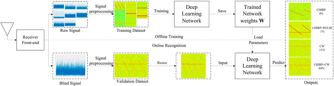
Figure 9. Detection and recognition process.

Interference detection and recognition primarily consist of two steps: offline training and real-time recognition. In the offline training phase, the receiver first collects signals via the antenna and transmits them to the front end of the receiver to generate raw sampled data. The sampled data is then preprocessed to construct a training dataset. Finally, the training data is input into the neural network for training, and the resulting network weights are saved. In the real-time recognition phase, the receiver antenna collects unknown signals, transmits them to the front end, and generates raw data. The data is then preprocessed, and its image dimensions are adjusted to meet the requirements of the neural network input. Finally, the processed data is input into the neural network, the weights saved from the offline training phase are loaded, and the classification results of the interference signal are output.

4.1 Simulated dataset

At the receiver front end, GNSS signals are first converted down to an intermediate frequency, then sampled into a digital sequence and finally sent to the acquisition and tracking module (Ferre et al., 2019). The received signal is represented as:

$x\left(t\right)={\displaystyle \sum _{i=1}^M}{s}_i\left(t\right)+n\left(t\right)+j\left(t\right)(15)$

where $M$ is the number of observed satellites, $s_i\left(t\right)n\left(t\right)$ $j\left(t\right)$ represent the signal from the $ith$ satellite, zero-mean Gaussian white noise with variance ${\sigma }_n^2$ , and jamming signal. Based on the investigation of interference source parameter settings both domestically and internationally, as well as a literature review, the simulated dataset in this paper generates B3I-type navigation signals with an initial code phase of 1,000 and a signal-to-noise ratio (SNR) set to −26 dB. The parameter ranges for the interference are shown in Table 2.

Table 2

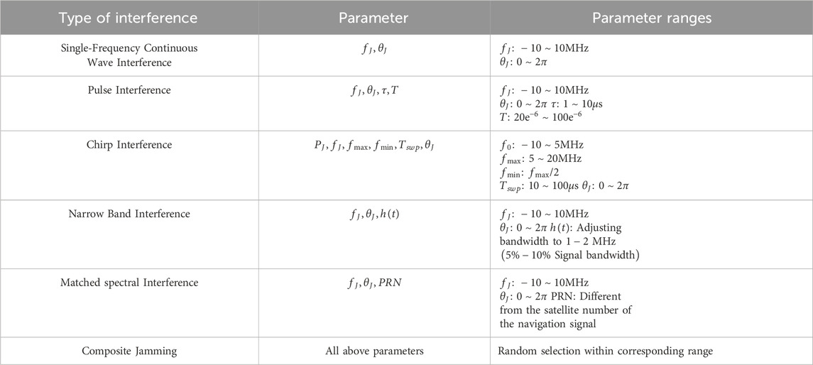
Table 2. Interference parameter settings.

The sampling rate is set to 21 MHz, the sampling time is 2 ms, and the JNR is set to −21–27 dB. Based on the above parameters and model, a simulated signal dataset is generated, followed by image datasets for each preprocessing method. The interference signals in the dataset include 16 types: 5 single interference types, 10 composite interferences combining two different interference types, and 1 case without interference. The JNR is set to range from −21 to −13 dB, with increments of 1 dB (as the detection probability and recognition accuracy vary significantly at lower JNR levels). Once the detection probability and recognition accuracy stabilize, the JNR is set from −12–27 dB with increments of 3 dB, resulting in 23 total JNR cases. For each JNR, 400 images are generated, with the validation, test, and training sets split in a ratio of 1:2:7. Specifically, for each JNR, 40 images are allocated to the validation set, 80 images to the test set, and 280 images to the training set.

4.2 Neural network and deep learning environment

This section focuses on the impact of preprocessing methods on interference detection and recognition performance. Therefore, a neural network that balances accuracy and parameter size should be selected. Figure 10 illustrates the relationship between recognition accuracy and GPU parameters for various neural networks used in image recognition. It is evident that the ResNet-18 network strikes a balance between image recognition speed and accuracy, achieving relatively short runtimes and high recognition rates (Sunnetci et al., 2023). Therefore, ResNet-18 is chosen as the standard neural network in this section. The network structure of ResNet-18 is shown in Figure 11.

Figure 10

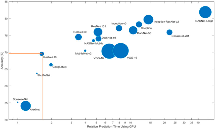
Figure 10. Recognition accuracy and speed of different neural networks.

Figure 11

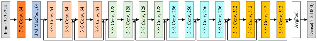
Figure 11. ResNet-18.

ResNet-18 consists of 17 convolutional layers, 1 dense layer, and additional layers such as pooling layers, batch normalization layers, and activation functions. The roles of these layers are as follows.

(1) Convolutional Layer: Convolutional layers perform the cross correlation operation to extract features and yield the feature map. The process is achieved by sliding a window, called the convolutional kernel, across the input matrix to compute an element-wise multiplication and sum up the result.

(2) Pooling Layer: Pooling layers perform the down sampling operation to further aggregate features. Unlike the convolutional operator with learnable parameters, the pooling operator is deterministic and typically calculates either the maximum or average value of elements in the pooling window.

(3) Batch Normalization Layer: Batch normalization layers are generally implemented after convolutional layers or pooling layers. It normalizes the inputs by subtracting their mean and dividing by their standard deviation, leading to faster training and less overfftting for deep networks.

(4) Activation Function: The objective of activation functions is to decide whether a neuron should be connected to the next layer.

(5) Dense Layer: Dense layer, also referred to as the fully connected layer, is the last layer of the network and plays the role of classification.

The training process was conducted using 50 iterations, with a learning rate set to 0.001 and a batch size of 64. An Nvidia Tesla V100 GPU was employed to accelerate computation. The hardware setup included an Intel^® Xeon^® Gold 6234 CPU operating at 3.30 GHz and an Nvidia Tesla V100 GPU, running on a Linux operating system. The software environment was configured with g++ and gcc compilers, along with CUDA 11.6 and PyTorch 2.0.0 as the deep learning framework.

4.3 Analysis of interference detection and recognition performance under different signal preprocessing methods

4.3.1 Performance analysis of detection and recognition

The results indicate that the detection rates of the time-frequency diagram and the power spectrum are comparable, both outperforming the histogram in detection performance. At a detection rate threshold of 90%, the sensitivity of time-frequency detection is approximately −20 dB, while spectrum detection achieves a sensitivity of −19 dB. In contrast, the histogram detection exhibits significantly lower sensitivity, approximately −3 dB. The relationship between detection probability and JNR is illustrated in Figure 12.

Figure 12

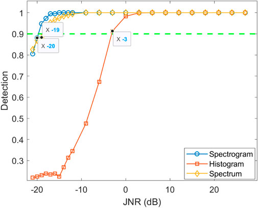
Figure 12. Relationship between detection probability and JNR.

The results demonstrate that the average recognition accuracy of the time-frequency diagram is marginally higher than that of the spectrum diagram and substantially higher than that of the histogram. At a recognition accuracy threshold of 90%, the sensitivity of the time-frequency recognition method is −13 dB, while the spectrum recognition method achieves a sensitivity of approximately −9 dB. In contrast, the histogram method achieves a maximum recognition accuracy of only 77.4%, reflecting a higher false detection rate and greater susceptibility to confusion between interference types. The relationship between recognition accuracy and JNR is depicted in Figure 13.

Figure 13

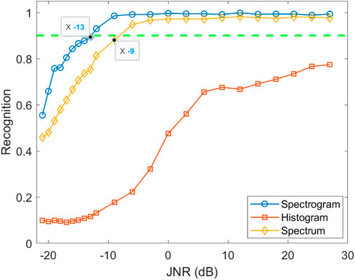
Figure 13. Relationship between recognition probability and JNR.

4.3.2 Analysis of the recognition of different types of interference using different preprocessing methods

4.3.2.1 Histogram

Experimental results indicate that in single interference recognition using histograms, the recognition accuracy for NB, PULSE, and MATCH interference approaches 100% only at high JNR levels. When the recognition accuracy reaches 90%, their sensitivity levels are 0, 3, and 18 dB, respectively. In contrast, the recognition accuracy for CW and CHIRP interference remains low. The relationship between the recognition accuracy of single interference using histograms and JNR is shown in Figure 14A. The recognition accuracy for NB, PULSE, and MATCH interference generally increases, while the accuracy for CHIRP and CW interference fluctuates significantly. At the same JNR, when CHIRP interference achieves relatively high recognition accuracy, CW interference has lower accuracy, and vice versa. This indicates that CHIRP and CW interference are prone to mutual confusion during recognition.

Figure 14

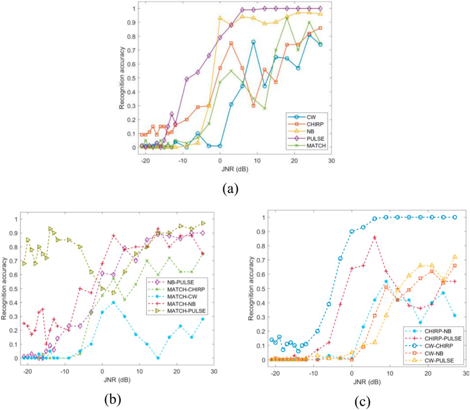
Figure 14. Relationship between recognition accuracy of interference and JNR using histograms. (a) Single interference. (b) and (c) composite interference.

In composite interference recognition, CW-CHIRP, NB-PULSE, MATCH-PULSE, and MATCH-NB achieve relatively high recognition accuracy. When their recognition accuracy reaches 90%, their sensitivity levels are 0, 15, 3, and 15 dB, respectively. The recognition accuracy for the remaining interference types is suboptimal. The confusion matrix at a JNR of 6 dB is shown in Figure 15.

Figure 15

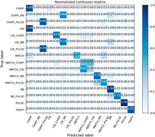
Figure 15. The confusion matrix of the histogram at a JNR of 6 dB.

From the confusion matrix, it can be observed that the reason for the low recognition accuracy of certain composite interferences is their combination with either CW or CHIRP interference. For example, CHIRP-NB is misclassified as CW-NB interference, and MATCH-CHIRP is misclassified as MATCH-CW interference. This is because the histogram features of CW and CHIRP are similar. The fundamental reason is that during signal generation, CHIRP interference is created by linearly varying the frequency of CW, which does not affect its time-domain statistical characteristics. The recognition accuracy-JNR plot for composite interference using histograms is shown in Figures 14B, C.

4.3.2.2 Power spectral density

Experimental results show that in single interference recognition, the recognition accuracy increases with the JNR, and NB interference exhibits higher recognition accuracy at low JNR levels. The JNR sensitivity for the five types of single interference when the recognition accuracy reaches 90% is as follows: PULSE, NB, CW: -9 dB; CHIRP, MATCH: -6 dB. The relationship between recognition accuracy for single interference and JNR is shown in Figure 16A.

Figure 16

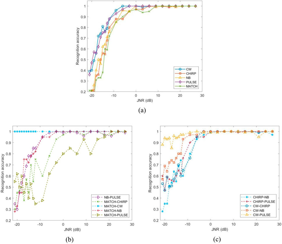
Figure 16. Relationship between recognition accuracy of interference and JNR using PSD. (a) Single interference. (b) and (c) composite interference.

Experimental results indicate that at low JNR levels, CW-PULSE and CW-MATCH exhibit superior recognition performance. At a JNR of −20 dB, their recognition accuracy reaches 94% and 100%, respectively, significantly higher than other types of composite interference. For the remaining composite interferences, the JNR sensitivity when the recognition accuracy reaches 90% is as follows: CW-NB: -12 dB; CHIRP-PULSE, NB-PULSE, MATCH-NB: -9 dB; CHIRP-NB, CW-CHIRP: -6 dB; MATCH-CHIRP: -3 dB; MATCH-PULSE: 9 dB. Among them, MATCH-PULSE is often misclassified as MATCH interference during recognition. The relationship between the recognition accuracy of composite interference using PSD and JNR is shown in Figures 16B, C.

4.3.2.3 Time-frequency diagram

In single interference recognition, under the threshold condition of achieving a recognition accuracy of 90%, the JNR sensitivities for the five types of single interference are as follows: PULSE: -19 dB, NB: -17 dB, CW and CHIRP: -16 dB, MATCH: -3 dB. As the JNR increases, the recognition accuracy for single interference shows a consistent upward trend, eventually approaching 100%. The relationship between the recognition accuracy of single interference using time-frequency diagrams and JNR is shown in Figure 17A.

Figure 17

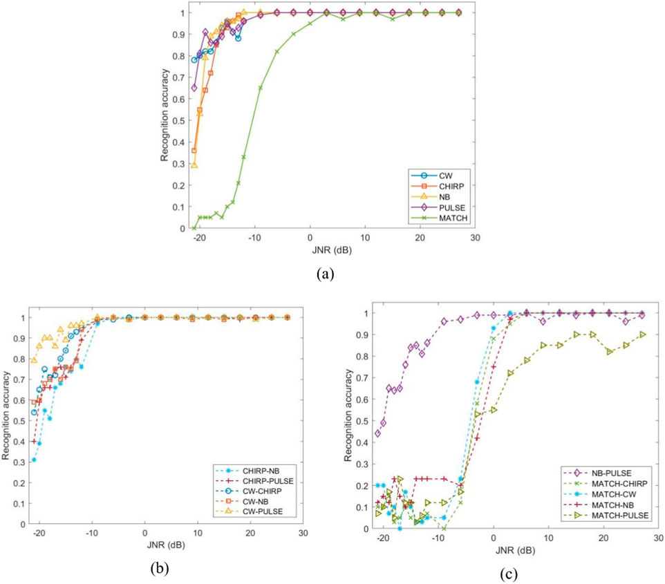
Figure 17. Relationship between recognition accuracy of interference and JNR using time frequency diagram. (a) single interference. (b) and (c) composite interference.

During the recognition of composite interference, CW-PULSE interference exhibits higher recognition accuracy at low JNR levels. When the recognition accuracy reaches 90%, the JNR sensitivities for ten types of composite interference are as follows: CW-PULSE: -19 dB, CW-CHIRP: -14 dB, CW-NB and CHIRP-PULSE: -12 dB, NB-PULSE and CHIRP-NB: -9 dB, MATCH-CW: 0 dB, MATCH-CHIRP and MATCH-NB: 3 dB, MATCH-PULSE: 15 dB. The results indicate that in single interference recognition, MATCH has the weakest recognition performance. When combined with other single interference types to form composite interference, the recognition performance of the resulting composite interference types is also suboptimal. In contrast, CW and PULSE achieve the best recognition accuracy in single interference recognition, and CW-PULSE also performs the best in composite interference recognition. It can be inferred that the time-frequency spectrogram of composite interference is the superposition of the corresponding single interference spectrograms. Therefore, the recognition accuracy of composite interference aligns with the trends of its constituent single interference recognition accuracy. The recognition accuracy-JNR plot for composite interference using time-frequency diagrams is shown in Figures 17B, C.

His section compares the performance of three signal preprocessing methods in interference detection and recognition. The results indicate that the data preprocessing methods generating time-frequency diagrams and PSD plots achieve similar detection and recognition performance, which is higher than that of histograms. Furthermore, the interference detection and recognition results were quantitatively analyzed, and the detection sensitivity for different methods was obtained. In the next step, the conclusions of this chapter will be used to integrate the preprocessing methods with better performance to further improve interference detection and recognition performance.

5 Low-complexity detection and recognition method for GNSS composite interference

Traditional interference recognition methods include threshold detection, spectral analysis, decision trees, and support vector machines (SVMs). These approaches typically rely on signal processing techniques and statistical analysis for manual feature extraction, resulting in lower recognition accuracy and sensitivity in complex interference scenarios. In contrast, deep learning methods leverage automatic feature extraction, offering higher recognition accuracy, better adaptability to complex interference environments, and the ability to handle nonlinear relationships between signals. The recognition accuracy and sensitivity of various methods are shown in Figure 18.

Figure 18

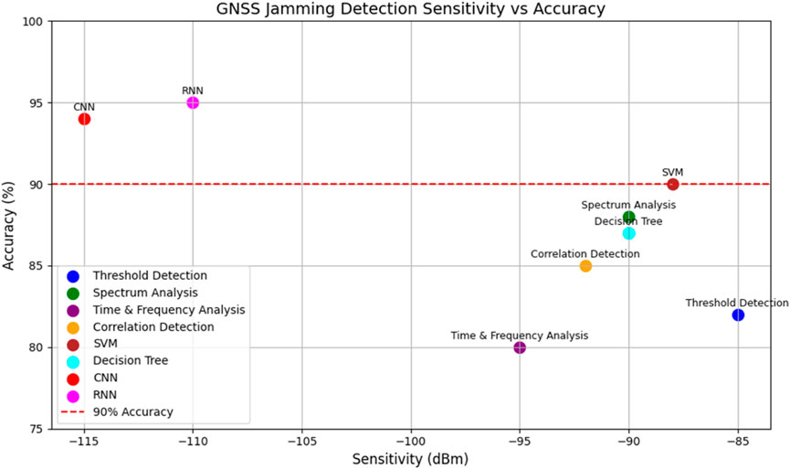
Figure 18. Average recognition accuracy and sensitivity of different methods for GNSS jamming.

Existing CNN-based interference classification techniques mostly adopt typical CNNs (AlexNet, ResNet-18, VGG-11) as classifiers. These networks are specifically designed for the ImageNet dataset and are not well-suited for interference recognition tasks, resulting in suboptimal performance. Another drawback of typical CNNs is that they contain numerous convolutional layers, leading to large data sizes and significant memory usage when deployed on terminal devices. Based on the dataset and hardware setup from the previous chapter, calculations show that the initial ResNet-18 network requires 42.67 MB of parameters, has a forward processing time of 1.43 s, and can process one image every 1.63 milliseconds on average. To achieve model light-weighting, this paper reduces the number of convolutional layers in typical CNNs, addressing their large number of convolutional layers, and designs the LcxNet network to reduce processing time. The architecture of the LcxNet network is shown in Figure 19.

Figure 19

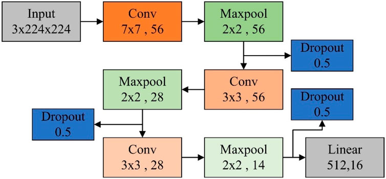
Figure 19. LcxNet architecture.

This network employs only three convolutional layers and three pooling layers, significantly reducing the number of parameters and computational complexity compared to deep networks like ResNet-18. This makes it more suitable for devices with limited computational resources. Additionally, the use of a 7 × 7 large kernel convolution for initial feature extraction effectively expands the receptive field and enhances information extraction efficiency, thereby reducing the need for deeper layers.

The first layer utilizes a 7 × 7 large kernel convolution (56 channels) for preliminary feature extraction, followed by a 2 × 2 max pooling operation to reduce data dimensionality and improve computational efficiency. Subsequently, a 3 × 3 small kernel convolution (56 channels) is applied to extract local details, followed by another pooling operation to further reduce computation. The final layer employs a 3 × 3 small kernel convolution (28 channels) to extract deeper features, combined with 2 × 2 max pooling to further compress the data volume, providing a refined feature representation for the fully connected layer. This network incorporates a multi-layer Dropout (0.5) mechanism, inserting Dropout after pooling layers to prevent overfitting and enhance the model’s generalization ability. Dropout is mainly applied to feature-rich layers to avoid redundancy and improve model stability. After feature extraction through convolutional and pooling layers, a 512-dimensional fully connected layer is used for feature fusion, ultimately mapping to an 16-dimensional output layer, making it suitable for 16-class classification tasks. Compared to ResNet-18, this network significantly reduces the number of parameters and computational complexity, making it more suitable for embedded and edge computing devices, particularly for real-time interference detection in complex electromagnetic environments.

After using the LcxNet network, the parameter size is reduced to 12.36 MB, the forward processing time is shortened to 1.21 s, and the network can process one image every 1.38 milliseconds, achieving a 15% improvement in recognition speed. This demonstrates that reducing the number of convolutional layers can significantly decrease network parameters and processing time, but it also leads to a notable reduction in detection and recognition accuracy to improve the interference detection and recognition rate based on this model, the study proposes a method of concatenating feature values obtained from different preprocessing methods after convolutional layers. Additionally, to further reduce model parameters, depthwise separable convolution is adopted in the original convolution module, making the network more light-weight.

In standard convolution operations, for an input tensor $H\times W\times C_{in}$ with height $H$, width $W$, and $C_{in}$ input channels, we typically use $C_{out}$ convolutional filters, each of size $K\times K$. The total number of parameters $P_n$ in a standard convolution is:

$P_n=H\times W\times K^2\times C_{in}\times C_{out}(16)$

The total computational cost arises because each pixel undergoes convolution with all filters. In contrast, depthwise separable convolutions decompose standard convolution into two independent steps:

• Depthwise Convolution: This operation applies a separate convolution filter to each input channel individually, without mixing information between channels. Each channel has its own $K\times K$ kernel, but there is no cross-channel interaction.

• Pointwise Convolution: A $1\times 1$ convolutional kernel (size: $1\times 1\times C_{in}\times C_{out}$) is used to combine information across different channels. This operation linearly combines the outputs of the depthwise convolution, effectively merging multiple input channels into new output channels. By separating spatial and channel-wise processing, this method significantly reduces both the parameter count and computational complexity compared to standard convolutions. The total computational cost of depthwise separable convolutions $P_s$ is given by:

$\begin{array}{l}{P}_s=H\times W\times K^2\times C_{in}+H\times W\times C_{in}\times C_{out}\\ =H\times W\times \left(K^2\times C_{in}+C_{in}\times C_{out}\right)\end{array}(17)$

Its computational cost is significantly lower than that of traditional convolutional blocks:

$\begin{array}{l}\frac{P_s}{P_n}=\frac{H\times W\times \left(K^2\times C_{in}+C_{in}\times C_{out}\right)}{H\times W\times K^2\times C_{in}\times C_{out}}\\ =\frac{1}{C_{out}}+\frac{1}{K^2}\end{array}(18)$

As a result, the LcxNet-Fusion network is designed. This network uses time-frequency diagrams and power spectral density plots, which have better interference recognition performance, as inputs. The two network models are concatenated to achieve feature fusion. The architecture of the LcxNet-Fusion network is shown in Figure 20.

Figure 20

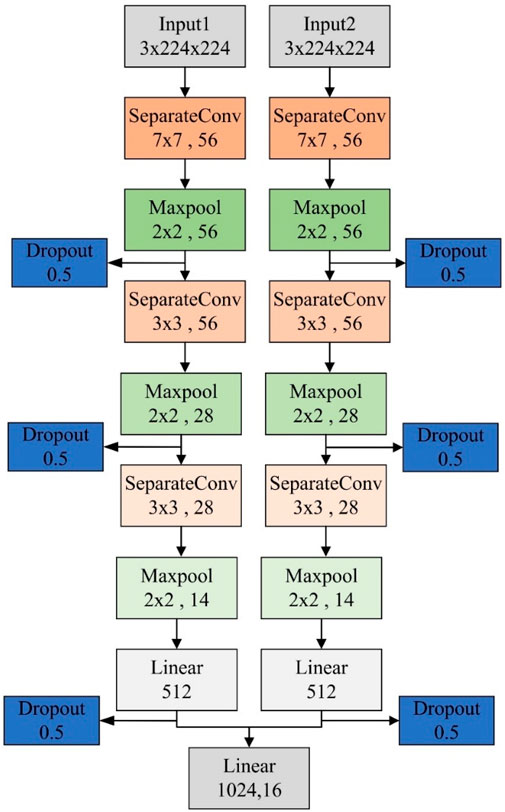
Figure 20. LcxNet-fusion architecture.

After using LcxNet-Fusion, the network parameter size is reduced to 24.32 MB, and the forward processing time is 1.25 s, with an average recognition time of 1.4 ms per image. While the recognition accuracy is slightly lower compared to ResNet-18, the accuracy under low signal-to-noise ratio conditions is significantly higher than that of the LcxNet network. The recognition accuracy of the three networks under varying signal-to-noise ratios is shown in Figure 21.

Figure 21

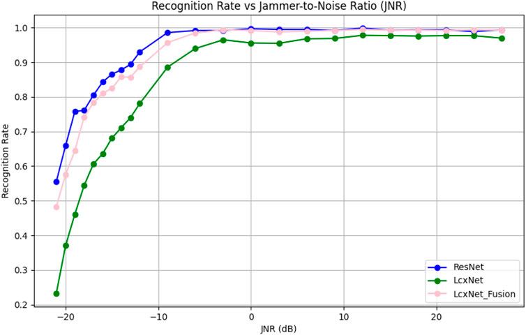
Figure 21. Comparison of recognition accuracy among three networks.

To verify the effectiveness of the deep learning network used in this study for interference detection and recognition, we provide a comparison of existing detection and recognition methods, as shown in Table 3, along with their corresponding JNR values at which they achieve a detection and recognition accuracy of 90%.

Table 3

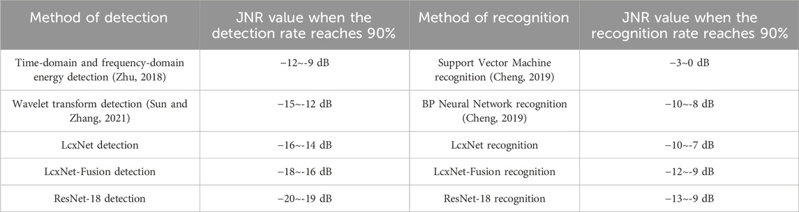
Table 3. Comparison of existing interference detection and recognition methods.

6 Conclusion

This study focuses on the detection and recognition of composite interference. Using various signal preprocessing methods, we analyzed the detection and recognition of composite interference and obtained quantitative conclusions. Furthermore, we developed the LcxNet-Fusion network, which reduces the parameter size within an acceptable range of accuracy loss. This study addresses the limitations of existing interference detection and recognition methods, which mostly focus on single interference scenarios, and enables lightweight deployment on terminals. It lays the foundation for future research on suppressing composite interference in receivers. The specific contributions of this paper are as follows:

• A composite interference model and dataset were constructed, providing a foundation for future research on composite interference suppression and more efficient detection and recognition methods.

• The effects of three different signal preprocessing methods on the detection and recognition of composite interference were analyzed. Quantitative conclusions were drawn regarding the relationship between JNR and detection results for various interference types under each method.

• The LcxNet-Fusion network was developed to achieve a more lightweight model with improved real-time performance compared to the ResNet network.

To enhance the robustness of composite interference detection and recognition for application across various terminals, future research can be conducted in the following directions:

• Investigate the integration of other preprocessing methods to analyze the detection and recognition performance for specific types of interference and to construct a more robust network model.

• Design more interference combination scenarios to investigate the detection and recognition of composite interference integrating suppression and deception techniques.

Data availability statement

The raw data supporting the conclusions of this article will be made available by the authors, without undue reservation.

Author contributions

CL: Conceptualization, Data curation, Formal Analysis, Investigation, Software, Validation, Visualization, Writing – original draft, Writing – review and editing. BR: Conceptualization, Software, Validation, Writing – review and editing. YX: Conceptualization, Project administration, Writing – review and editing. FC: Project administration, Resources, Software, Supervision, Validation, Visualization, Writing – review and editing.

Funding

The author(s) declare that financial support was received for the research and/or publication of this article. This research was funded by the National Natural Science Foundation of China (U20A0193).

Acknowledgments

The authors would like to thank the editors and reviewers for their efforts to help the publication of this paper.

Conflict of interest

The authors declare that the research was conducted without any commercial or financial relationships that could be construed as a potential conflict of interest.

Generative AI statement

The author(s) declare that no Generative AI was used in the creation of this manuscript.

Publisher’s note

All claims expressed in this article are solely those of the authors and do not necessarily represent those of their affiliated organizations, or those of the publisher, the editors and the reviewers. Any product that may be evaluated in this article, or claim that may be made by its manufacturer, is not guaranteed or endorsed by the publisher.

References

Borio, D., Dovis, F., Kuusniemi, H., and Presti, L. L. (2016). Impact and detection of GNSS jammers on consumer grade satellite navigation receivers. Proc. IEEE 104, 1233–1245. doi:10.1109/jproc.2016.2543266

CrossRef Full Text | Google Scholar

Buesnel, G. (2018). Expect your GPS to Be trashed, GPS and ADS-B problems at manila airport. RNT Foundation.

Google Scholar

Cheikh, K., and Soltani, F. (2006). Application of neural networks to radar signal detection in K-distributed clutter. IEE Proc. Radar Sonar Navig. 153, 460–466. doi:10.1049/ip-rsn:20050103

CrossRef Full Text | Google Scholar

Cheng, W. (2019). Research on interference identification technology in satellite communication systems [Doctoral dissertation, Xidian University]. Xidian Univ.

Google Scholar

Chralampidis, D., Kasparis, T., and Georgiopoulos, M. (2001). Classification of noisy signals using fuzzy ARTMAP neural networks. IEEE Trans. Neural Netw. 12, 1023–1036. doi:10.1109/72.950132

PubMed Abstract | CrossRef Full Text | Google Scholar

Darzikolaei, M. A., Ebrahimzade, A., and Gholami, E. (2015). “Classification of radar clutters with artificial neural network,” in Proceedings of the 2nd International Conference on Knowledge-Based Engineering and Innovation (KBEI), Tehran, Iran, 5–6 November 2015 (IEEE), 577–581.

CrossRef Full Text | Google Scholar

Ferre, R. M., Fuente, A. D. L., and Lohan, E. S. (2019). Jammer classification in GNSS bands via machine learning algorithms. Sensors 19, 22. doi:10.3390/s19224841

CrossRef Full Text | Google Scholar

R. N. T. Foundation (2017). Russian exercise jams aircraft GPS in north Norway for a week—NRK translated from Norwegian, RNT foundation.

Google Scholar

He, K., Zhang, X., Ren, S., and Sun, J. (2016). “Deep residual learning for image recognition,” in Proceedings of the IEEE/CVF Conference on Computer Vision and Pattern Recognition (CVPR), Las Vegas, NV, USA, 27–30 June 2016, 770–778.

Google Scholar

Huang, Z., Kabán, A., and Reeve, H. (2024). Efficient learning with projected histograms. Data Min. Knowl. Discov. 38 (6), 3948–4000. doi:10.1007/s10618-024-01063-6

CrossRef Full Text | Google Scholar

Ibrahim, N., Abdullah, R., and Saripan, M. (2009). Artificial neural network approach in radar target classification. J. Comput. Sci. 5 (1), 23–32. doi:10.3844/jcssp.2009.23.32

CrossRef Full Text | Google Scholar

Jeong, S., Kim, M., and Lee, J. (2020). CUSUM-based GNSS spoofing detection method for users of GNSS augmentation system. Int. J. Aeronaut. Space Sci. 21, 513–523. doi:10.1007/s42405-020-00272-9

CrossRef Full Text | Google Scholar

Kraus, T., Bauernfeind, R., and Eissfeller, B. (2011). “Survey of in-car jammers—analysis and modeling of the RF signals and IF samples (suitable for active signal cancelation),” in Proceedings of the 24th International Technical Meeting of The Satellite Division of the Institute of Navigation (ION GNSS 2011), Portland, OR, USA, September 2011, 20–23.

Google Scholar

Krizhevsky, A., Sutskever, I., and Hinton, G. E. (2012). ImageNet classification with deep convolutional neural networks. Commun. ACM 60, 84–90. doi:10.1145/3065386

CrossRef Full Text | Google Scholar

Macii, A., Macii, E., Poncino, M., and Scarsi, R. (2001). Stream synthesis for efficient power simulation based on spectral transforms. IEEE Trans. Very Large Scale Integr. (VLSI) Syst. 9, 417–426. doi:10.1109/92.929576

CrossRef Full Text | Google Scholar

Sakorn, C., and Supnithi, P. (2021). “Calculating AGC and C/N₀ thresholds of mobile for jamming detection,” in Proceedings of the 2021 18th International Conference on Electrical Engineering/Electronics, Computer, Telecommunications and Information Technology (ECTI-CON), Thailand, 24–27 May 2021 (Chiang Mai).

Google Scholar

Simonyan, K., and Zisserman, A. (2015). “Very deep convolutional networks for large-scale image recognition,” in Proceedings of the 3rd International Conference on Learning Representations (ICLR), San Diego, CA, USA, 7–9 May 2015, 1–14.

Google Scholar

Sun, K., and Zhang, T. (2021). A new GNSS interference detection method based on rearranged wavelet–Hough transform. Sensors 21, 1714. doi:10.3390/s21051714

PubMed Abstract | CrossRef Full Text | Google Scholar

Sunnetci, K. M., Kaba, E., Çeliker, F. B., and Alkan, A. (2023). Comparative parotid gland segmentation by using ResNet-18 and MobileNetV2 based DeepLab v3+ architectures from magnetic resonance images. Concurr. Comput. Pract. Exp. 35, e7405. doi:10.1002/cpe.7405

CrossRef Full Text | Google Scholar

Wang, A., Zhu, T., and Meng, Q. (2024). Spectrum sensing method based on STFT-RADN in cognitive radio networks. Sensors 24, 5792. doi:10.3390/s24175792

PubMed Abstract | CrossRef Full Text | Google Scholar

Wang, H., and Jiang, Y. (2018). Real-time parameter estimation for SAR moving target based on WVD slice and FrFT. Electron. Lett. 54, 47–49. doi:10.1049/el.2017.1740

CrossRef Full Text | Google Scholar

Wang, Y., Liu, Y., Roesler, C., and Morton, Y. J. (2020). “Detection of coherent GNSS-R measurements using a support vector machine,” in Proceedings of the IGARSS 2020—2020 IEEE International Geoscience and Remote Sensing Symposium, Waikoloa, HI, USA, 26 September–2 October 2020.

Google Scholar

Wei, M., and Mo, Z. (2025). Multireassignment method based on S-transform for time-frequency analysis of nonstationary signal. IEEE Sens. J. 25, 3110–3118. doi:10.1109/jsen.2024.3506784

CrossRef Full Text | Google Scholar

Yin, H., Chen, H., Feng, Y., and Zhao, J. (2023). Time-frequency-energy characteristics analysis of vibration signals in digital electronic detonators and nonel detonators exploders based on the HHT method. Sensors 23, 5477. doi:10.3390/s23125477

PubMed Abstract | CrossRef Full Text | Google Scholar

Yleisradio, Y. (2018). Russia suspected of GPS jamming during nato exercises. Finnair reports GPS jamming near Kaliningrad. Yle

Google Scholar

Yuan, Y., Wang, L.-N., Zhong, G., Gao, W., Jiao, W., Dong, J., et al. (2022). Adaptive gabor convolutional networks. Pattern Recognit. 124, 108495. doi:10.1016/j.patcog.2021.108495

CrossRef Full Text | Google Scholar

Zhang, J., Li, H., Yang, X., Cheng, Z., Zou, P. X. W., Gong, J., et al. (2024). A novel moisture damage detection method for asphalt pavement from GPR signal with CWT and CNN. NDT E Int. 145, 103116. doi:10.1016/j.ndteint.2024.103116

CrossRef Full Text | Google Scholar

Zhu, P. (2018). GNSS interference detection and recognition technology research [Doctoral dissertation, Chongqing University]. Chongqing Univ.

Google Scholar

Zhu, W., Sice, P. V., Zhang, W., Krajewska, K., and Zhao, Z. (2024). Parallels between the physical vacuum and concept of qi in medical qigong: comprehending oneness. Kybernetes. doi:10.1108/k-04-2024-1087

CrossRef Full Text | Google Scholar