 Riccardo Simionato
 Stefano Fasciani
- Department of Musicology, University of Oslo, Oslo, Norway
This article introduces a novel method for emulating piano sounds. We propose to exploit the sine, transient, and noise decomposition to design a differentiable spectral modeling synthesizer replicating piano notes. Three sub-modules learn these components from piano recordings and generate the corresponding quasi-harmonic, transient, and noise signals. Splitting the emulation into three independently trainable models reduces the modeling tasks’ complexity. The quasi-harmonic content is produced using a differentiable sinusoidal model guided by physics-derived formulas, whose parameters are automatically estimated from audio recordings. The noise sub-module uses a learnable time-varying filter, and the transients are generated using a deep convolutional network. From singular notes, we emulate the coupling between different keys in trichords with a convolutional-based network. Results show the model matches the partial distribution of the target while predicting the energy in the higher part of the spectrum presents more challenges. The energy distribution in the spectra of the transient and noise components is accurate overall. While the model is more computationally and memory efficient, perceptual tests reveal limitations in accurately modeling the attack phase of notes. Despite this, it generally achieves perceptual accuracy in emulating single notes and trichords.
1 Introduction
Piano sound synthesis is a challenging problem and is still a topic of great interest. Historically, accurate piano models have been developed mainly using physical modeling techniques (Chabassier et al., 2014), which are required to discretize and solve partial differential equations. This approach leads to significant computational challenges. Recently, neural-based approaches, based on autoregressive architecture (Hawthorne et al., 2019) or Differentiable Digital Signal Processing (DDSP) framework (Engel et al., 2020), have produced convincing audio signals. In particular, the DDSP framework, which involves integrating machine learning techniques into digital signal processors, has been mainly explored. Among traditional synthesis algorithms, DDSP has been integrated with wavetable (Shan et al., 2022) and frequency modulation (FM) (Caspe et al., 2022) synthesis. DDSP allows data generation conditioned by MIDI information, specifically generating parameters used for digital signal algorithms. DDSP has also been used with Spectral Modelling Synthesis (Serra and Smith, 1990) (SMS), which considers the sound signal as the sum of harmonic and noise parts. The harmonic content can be synthesized with a sum of sine waves whose parameters are directly extrapolated from the target. The noise is usually approximated with white noise processed with a time-varying filter. This method has been applied to (Kawamura et al., 2022) for a mixture of harmonic audio signals, guitar (Wiggins and Kim, 2023; Jonason et al., 2023), and piano synthesis (Renault et al., 2022). The method has been extended considering transients for the case of sound effects (Liu et al., 2023) and percussive sound synthesis (Shier et al., 2023). In the first-mentioned work (Liu et al., 2023), the transients are synthesized using the discrete cosine transform (DCT) (Verma and Meng, 2000), transforming an impulse signal in a sine wave. The authors synthesized the transient by learning the amplitudes and frequencies of its discrete cosine transforms and synthesized it using sinusoidal modeling. In the second work (Shier et al., 2023), the transients are added to the signal using a Temporal convolutional neural network. In the reviewed works, audio is mostly generated with a sampling frequency of 16 kHz, except in (Liu et al., 2023; Jonason et al., 2023), where the sampling rates are 22.5 and 48 kHz, respectively.
Artificial neural networks can learn complex system behaviors from data, and their application for acoustic modeling has been beneficial. Differentiable synthesizers aiming to synthesize acoustic instruments have already been proposed, but, as we have previously detailed, reviewed studies on guitar and piano neural synthesis employ models that learn from datasets filled with recorded songs and melodies. This approach increases the complexity of the tasks and can limit the network’s ability to generalize, leading to challenges in scenarios not represented in the datasets. One example is the reproduction of isolated individual notes, where other concurrent sonic events might obscure the harmonic content of single notes in the dataset. Consequently, neural networks require a large amount of internal trainable parameters and training data to learn these complex patterns.
The work we detail in this paper extends our prior proposal for modeling the quasi-harmonic contents of piano notes (Simionato et al., 2024), and faces the problem from another perspective. We address the mentioned shortcoming by first emulating individual piano notes and then by incorporating the effects of key coupling, re-striking of played keys, and other scenarios that could occur during a real piano performance. Here, we combine the Differentiable Digital Signal Processing (DDSP) approach with the sines, transients, and noise (STN) decomposition (Verma and Meng, 2000) to synthesize the sound of individual piano notes, while a convolutional-based network is employed to emulate trichords. The generation of the notes is guided by physics knowledge, which allows designing a model with significantly fewer internal parameters. In addition, the model predicts a few audio samples at a time, allowing interactive low-latency implementations. The long-term objective of this research is to develop novel approaches for piano emulation that improve fidelity compared to existing techniques and are less computationally expensive than physical modeling while requiring less memory than sample-based methods.
Our approach includes three sub-modules, one for each component of the sound: quasi-harmonic, transient, and noise. The quasi-harmonic component corresponds to the partials during the quasi-stationary part of the note, which decays exponentially. The transient component, also referred to as percussive (Driedger et al., 2014), refers to the initial, inharmonic, and percussive portion produced by the hammer strike, which decays rapidly. Lastly, the noise component is the residual from the decomposition process, which, in the case of piano notes, can be associated with background noise and friction sound arising from internal mechanisms, such as the movements of the hammer and key.
The quasi-harmonic component is modeled using differentiable spectral modeling to synthesize the sines waves composing the sound. The quasi-harmonic module, guided by physics formulas, predicts the inharmonic factor to produce the characteristic inharmonicity of the piano sound and the amplitude’s envelope for each partial. The model also considers phantom partials, beatings, and double decay stages. The transients are modeled by generating a sine-based waveform that is transformed using the Inverse Discrete Cosine Transform (IDCT), producing the impulsive component of the sound. The vector of samples representing the waveform is computed entirely using a convolutional-based neural network. Finally, the noise component is synthesized filtering in the frequency domain of a Gaussian noise signal. The noise sub-model predicts the coefficients of the noise filter. Once the notes are computed, we emulate the coupling between different keys for trichords. A convolutional neural network processes the sum of individual note signals to emulate the sound of real chords.
The approach synthesizes the notes separately, removing the need to have a large network learning how to synthesize all the notes using the same parameters. In this way, we need one model per key, similar to the sample-based methods, but we need to store a few parameters without storing the audio. Interpolation between different velocities, which indicate the speed and force with which a key is pressed to play a note, is also automatically modeled. This does not preclude the modeling of coupling or re-striking of keys, which is not allowed by sample-based methods, by adding an additional small network and, in turn, without adding significant complexity as in physical modeling methods.
The rest of the paper is organized as follows. Section 2 describes the physics of the piano, focusing on aspects used to inform our model. Section 3 details our methodology, the architectures, the used datasets, and the experiments we have carried out. Section 4 summarizes and discusses the results we obtained, while Section 5 concludes the paper with a summary of our findings.
2 The piano
The piano is an instrument that produces sound by striking strings with hammers. When a key is pressed, a mechanism moves the corresponding hammer, usually covered with felt layers, to accelerate it to a few meters per second (1–6 m/s) before release. One important aspect of piano strings is the tension modulation. This modulation occurs due to the interaction between the string’s mechanical stretching and viscoelastic properties. It allows for shear deformation and changes in length during oscillation. These length changes cause the bridge to move sideways, which excites the string to vibrate in a different polarization. This vibration gains energy through coupling and induces the creation of longitudinal waves (Etchenique et al., 2015). Longitudinal motion (Nakamura, 1994; Conklin Jr, 1999) is also generated due to the string stretching during the collision with the hammer. When the hammer comes into contact with the string, it causes the string to elongate slightly from its initial length. This stretching creates longitudinal waves that propagate freely. The amplitude of these waves is relatively small compared to the transverse vibrations. The longitudinal vibration of piano strings greatly contributes to the distinctive character of low piano notes, and their properties and generation are not fully understood yet. They are named phantom partials and are generated by nonlinear mixing, and their frequencies are the sum or difference of transverse model frequencies. We can distinguish two types: even phantoms and odd phantoms. Even phantoms have double the frequency of a transverse mode, while odd ones have a frequency as the sum or difference of two transverse modes. Even and odd are pointed as the free and forced responses of the system (Bank and Sujbert, 2003).
Another important phenomenon in piano strings happens when keys feature multiple strings (Weinreich, 1977). Imperfections in the hammers cause the strings to vibrate with slightly varying amplitudes. In the case of two strings, they initially vibrate in phase, but each string loses energy faster than when it vibrates alone. As the amplitude of one string approaches zero, the bridge continues to be excited by the movement of the other string. As a result, the first string reabsorbs energy from the bridge, leading to a vibration of the opposite phase. This antiphase motion of the strings creates the piano’s aftersound. Any discrepancies in tuning between the strings contribute to this effect, together with the bridge’s motion, which can cause the vibration of one string to influence others. These phenomena affect the decay rates and produce the characteristic double decay. Similarly, the same effects can be caused by different polarizations in the string. Specifically, since the vertical polarization is greater than that one parallel to the soundboard, more energy is transferred to the soundboard, resulting in a faster decay. When the vertical vibrations are small, the horizontal displacement becomes more significant, producing double decay. In addition, the horizontal vibration is usually detuned with respect to the vertical one [
String stiffness leads to another significant aspect characterizing the piano sound: the inharmonicity of its spectrum (Podlesak and Lee, 1988). Specifically, the overtones in the spectra shift, so their frequencies do not have an integer multiple relationship. For this reason, they are called partials instead of harmonics. There are slightly different formulations of this aspect, which lead to different definitions of the inharmonicity factor
where
where
while
The soundboard damping is a linear phenomenon of modal nature, and the attenuation increases with the frequency of the modes (Ege, 2009). Therefore, the damping function is supposed to be increasing and have a sub-linear growth at infinity:
with
Lastly, aspects of sound radiation are not considered here and are left as a separate and independent modeling challenge. For this purpose, Renault et al. (2022) utilize a collection of room impulse responses, while recent advancements in neural approaches have also been explored (Mezza et al., 2024).
3 Methodology
The proposed modeling method presents three trainable sub-modules synthesizing different aspects of the piano sound. The respective quasi-harmonic, transient, and noise components extracted from real piano recordings are utilized to train the sub-modules separately. The sum of the signals generated by the three sub-modules represents the output of the model. Each sub-module is fed at the input with a vector, including the fundamental frequency and the velocity of the note to be synthesized. For the sub-models synthesizing the quasi-harmonic part and the noise, the input vector also includes an integer time index informing the model of the time elapsed from the note’s attack. The index expresses time in audio sampling periods, progressively incremented by the number of output audio samples predicted by each model’s inference. Including this time index is beneficial for the model as it simplifies the task of tracking the envelopes in the target sound. Note that the model learns to generate the sound of individual piano notes with the same duration found in the dataset, which generally includes recordings of keys held in the struck position until the sound has fully decayed. Shorter durations can be obtained by integrating an envelope generator as an additional damping module and leveraging its release stage.
3.1 Quasi-harmonic model
The architecture of the quasi-harmonic model is visible in Figure 1, while the layers composing it is in Figure 2. The quasi-harmonic model consists of 3 layers: the Inharmonicity layer, the Damping layer, and the Sine Generator layer. Physical information is embedded in the model when generating the note’s partials and envelope. The Sine Generator layer takes the partial frequency values and generates the corresponding sine waves. In the quasi-harmonic model, the learning is pursued using the multi-resolution Short-time Fourier Transform (STFT) loss and the Mean-Absolute-Error (MAE) of the Root-Mean-Square (RMS) energy computed per iteration, as similarly in (Simionato et al., 2024). The multi-resolution STFT loss is the average of STFT losses computed with window sizes of [256, 512, 1,024, 2,048, 4,096] and

Figure 1. The quasi-harmonic model consists of 3 layers: the Inharmonicity layer (a), the Damping layer (b), and the Sine Generator layer (c). The Inharmonicity layer computes the partial distribution for vertical and horizontal polarizations, the Damping layer predicts the partial amplitudes, while the Sine Generator layer computes and sums together all the sine components.
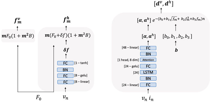
Figure 2. The layers composing the quasi-harmonic model. The Inharmonicity layer (left) takes the inharmonicity factor
3.1.1 Inharmonicity layer
The Inharmonicity layer adjusts the generation of partials based on the learnable inharmonicity factor
This approach provides an approximation to the inharmonic characteristics of the note. The tuning employs the Cent loss (Simionato et al., 2024), which takes into account the first 6 partials. The actual fundamental frequency
3.1.2 Damping layer
The Damping layer is based on the VC damping model. Partials exponentially decay over time as described by Equation 6:
where
where
where
where
where
where
The actual decay rate for each partial is generated using Equation 11, and the corresponding sine waves are synthesized as described in Equation 12:
The model can generate amplitude values for audio segments of any length without architectural constraints. Using lower sample numbers leads to reduced latency, longer training times, and increased computational costs per sample during inference. However, the accuracy of the results tends to improve, as this approach avoids additional artifacts by allowing the network to update the damping coefficients more frequently. The results presented in this paper pertain to the extreme case where the model generates a single sample per inference iteration.
3.2 Beatings and double decay
As mentioned in Section 2, piano strings present vertical and horizontal vibrations. The vibrations have different decay rates. The string exchanges energy with the bridge. The vertical vibration energy dissipates quickly, making up the initial fast decay. As the vertical displacement reduces, horizontal displacement becomes more dominant and exhibits the second slower decay. This created the so-called double decay, while the detuning between the two polarizations creates beatings. Similarly, the same effect can be created when the hammer strikes multiple strings. Strings in the same key cannot be perfectly in tune or slightly differently excited. The detuning creates out-of-phase vibrations that cancel each other out and reduce the energy exchange with the bridge. As before, it creates two different decaying rates and beatings.
This feature is integrated into the model, generating an additional set of partials. To account for the second polarization, the model employs a feedforward network consisting of two linear hidden layers with 8 units each. The first layer operates without activation functions, while the second utilizes the GELU activation function. Batch normalization is placed before the output layer with a single unit and the hyperbolic tangent as the activation function. The network predicts the detuning factor
3.3 Phantom partials
The model incorporates longitudinal displacements described in Section 2. Instead of employing a machine-learning approach, phantom partials are computed directly from the predicted transverse partials and their associated coefficients. Specifically, even phantom partials are obtained by doubling the frequencies of the two transverse polarizations and squaring their corresponding coefficients, as described by Equation 13
Note that doubling the partials leads to doubling the decay rates
where
3.4 Transient model
The architecture of the transient model is illustrated in Figure 3. We exploit the discrete cosine domain to synthesize the transients. In particular, we designed a deep convolutional oscillator to compute a sines-based waveform that will be converted using an inverse Discrete Cosine Transform (IDCT). Similarly to (Kreković, 2022), we designed a generative network based on a stack of upsampling and convolutional layers to generate the waveform from the frequency and velocity information. The model outputs an array of 1,300 samples representing the DCT waveform that is converted into the transient using the Equation 16:
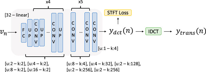
Figure 3. The transient model takes the velocity of the note as input and, using a stack of upsampling and convolutional layers, generates the waveform. The resulting waveform is inversely discrete cosine transformed to compute
The multi-resolution STFT loss function compares the output vector to the actual DCT signal from the dataset, using [32, 64, 128, 256] as window lengths. The input to the network is the velocity
3.5 Noise model
The architecture of the noise model is shown in Figure 4. The noise is modeled generating noise filter magnitudes
where
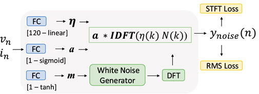
Figure 4. The noise is modeled generating noise filter magnitudes
To help the prediction, we also anchor the mean of the white noise signal to be generated. An FC layer with 1 unit and hyperbolic tangent activation predicts the mean of the white noise to be generated, and another FC layer with 1 unit and sigmoid activation computes the amplitudes of the noise signal. In this case, the MAE of the RMS is used as a loss function. The inputs of all the cases are a vector containing the velocity
3.6 Trichords
The coupling among different keys that happens during chords is modeled by a convolutional neural network and temporal Feature-wise Linear Modulation (FiLM) method (Birnbaum et al., 2019) followed by Gated Linear Unit (Dauphin et al., 2017) as in (Simionato and Fasciani, 2024), which conditions the network based on the playing keys. The input vector consists of the sum of the signals of the three generated notes, while the frequencies and velocities corresponding to the three notes, together with the time index
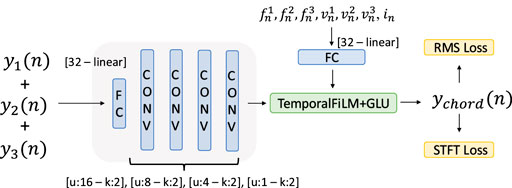
Figure 5. The coupling among different keys is modeled by a convolutional neural network and temporal FiLM method combined with the GLU to condition the network based on the keys playing. The input vector is the sum of the three separate note sounds, while their frequencies, velocities, and time index compose the conditioning vector.
3.7 Dataset
For this study, we use the BiVib dataset1, which includes piano sounds recorded from electro-mechanically actuated pianos controllable via MIDI messages. We selected the piano recordings related to the upright-closed and grand-open collection. For both collections, we also narrowed the recordings utilized to train the models to two octaves (C3 to B4), and we considered velocities between 45 and 127. Each recording in the dataset is associated not with a specific velocity value but rather with a velocity range, likely because small variations in velocity produce negligible changes in sound. For our experiments, we have associated each recording with the lower bound of its respective velocity range. This resulted in 168 note recordings with
where
We use all combinations derived from the 6 extrapolated partials to estimate
The transient and harmonic content of the notes were constructed using the Harmonic Percussive Source Separation (HPSS) method (Driedger et al., 2014) with a margin of 8. These separated components are considered the target of each sub-model. Once trained, the model will generate each component to be added to each other and reconstruct the original sound. The noise components were computed by subtracting the transient and harmonic spectrograms from the original note spectrogram. The DCT was also calculated from the transient component.
For the chords, we extended the dataset used in (Simionato et al., 2024) by including not only singular notes but also minor triads in the C3-B4 range, played at velocities of [60, 70, 80, 90, 100, 110, 120]. The input-output pair, in this case, is the sum of separate notes and the actual trichord recording.
3.8 Experiments setup
The models are trained using the Adam (Kingma and Ba, 2014) optimizer with a gradient norm scaling of 1 (Pascanu et al., 2013). The training was stopped earlier in case of no reduction of validation loss for 50 epochs, and the learning rate was reduced by
The datasets considering single notes are partitioned by key, with the middle velocity of 78 designated as the test set. On the other hand, in the trichords scenario, the dataset is split into
3.9 Perceptual evaluation
Perceptual evaluation is based on Multiple Stimuli test with Hidden Reference and Anchor (MUSHRA) (ITU-R, 2015), which is utilized to evaluate single notes and trichords generated by the proposed model. Usually, the MUSHRA test involves multiple trials. In each trial, the listener is requested to rate a set of signals on a scale 0 to 100 against a given reference signal. Each 20-point band on the scale is labeled with descriptors: excellent, good, fair, poor, and bad. Each trial requires participants to rate a set of signals, which includes the reference itself, known as the hidden reference, as well as one or more anchors. The hidden reference is used to identify clear and obvious errors. Indeed, data from listeners who rate the hidden reference lower than 90 for more than
The test consisted of 9 trials: in the first 6, participants rated single notes generated by the models trained with datasets from both an upright and a grand piano, with 3 trials dedicated to each. This was done to evaluate whether the model had successfully learned the characteristics of the specific target piano. In the last 3 trials, participants rated trichords to assess the model’s ability to emulate a realistic-sounding trichord. The models are trained on a dataset with notes ranging from
To assess the statistical significance of the MUSRA test results, we employ the Friedman test and the Cliff’s delta. The Friedman test evaluates the consistency of rankings assigned to the MUSHRA scores across different trials. Scores from each trial are ranked in ascending order; the lowest score receives a rank of 1, while the highest score is given a rank equal to the number of conditions evaluated in the trial. These ranks are used to calculate a test statistic, from which
MUSHRA tests are carried out in a controlled, quiet room, with participants using professional over-ear headphones, the Beyerdynamic DT-990 Pro, connected to the output of a MOTU M4 audio interface. Participants are provided with a browser-based Graphical User Interface (GUI) (Schoeffler et al., 2018) to facilitate the process of listening, comparing, and rating the audio signals. The 9 trials are conducted sequentially, in a fixed order, without interruption, and the total duration of the test, excluding the introduction and setup, is approximately 10 min.
3.10 Comparative evaluations
To further evaluate the approach, we employed the computational method proposed in Simionato and Fasciani (2023). We used the same audio descriptors in the proposal but are considering recording at 24,000 Hz. In particular, the method involves the Linear Discriminant Analysis (LDA) projection to maximize the separability between the types of pianos, acoustic, sample-based models, and physics-based models while minimizing within-type variance. LDA projects the feature vectors into a lower-dimensional space with dimensionality or a number of components equal to the number of classes minus one. A large set of audio descriptors are used to compute the feature vectors. For this paper, we considered two cases, the single note and trichord stimuli. For each type of stimulus, each feature vector is associated with a label representing the type of piano, acoustic or synthetic Pulse Code Modulation (PCM)-based or synthetic physics-based. For the single-note case, each vector is a high-dimensional representation of how the generated sound changes when increasing the velocity of the stimulus, while for the trichord case, each vector represents the difference between the sum of three notes and the actual trichord. For the single note case, we compute the dataset by creating a recording of sample-based and physical-based digital pianos, using the same velocities and the length of the dataset used for training our models. On the opposite, since the dataset used for training the trichord models uses the same sounds collected for the comparative study presented in Simionato and Fasciani (2023), we downsampled the original example to 24,000 Hz.
4 Results
Figure 6 shows the RMS and STFT losses for models of each key, also detailing losses for the quasi-harmonic, transient, and noise sub-models. The bar plot presents the STFT losses, normalized by the target spectrogram norm, as used for training the quasi-harmonic sub-module. The window resolutions utilized here are the same STFT resolutions used for the quasi-harmonic component. Generally, the model presents good accuracy considering all component-related losses. The models’ accuracy is also consistent in most of the keys across the octaves, except for
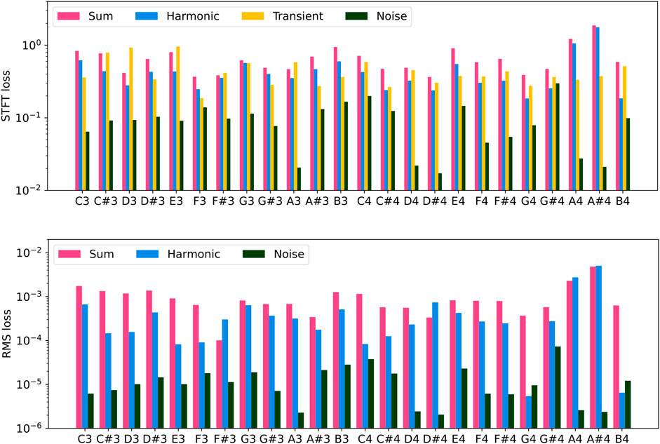
Figure 6. STFT (top) and RMS (bottom) losses of the test set across all the keys and considering the upright piano. STFT losses are normalized by the norm of the target spectrogram, as in the training process, and the window resolutions employed are identical to those used for the STFT of the quasi-harmonic component. The y-axis is on a logarithmic scale. Magenta bars refer to the sum of all components; blue bars refer to the quasi-harmonic component; the yellow bars refer to the transient component, and the dark green bars refer to the noise component.
Similar behavior is found when training the model with the grand piano dataset. In the bars plot of Figure 7, the RMS mismatch is considerably lower, but the STFT one is generally slightly bigger than the upright case. This may be due to the physics equations used for the partials’ decay envelope being intended for the grand piano case. The upright piano type could involve slightly different behaviors due to the different soundboards. In this case, there are no specific keys that appear to be more challenging for accurate modeling, unlike the situation with the upright piano.
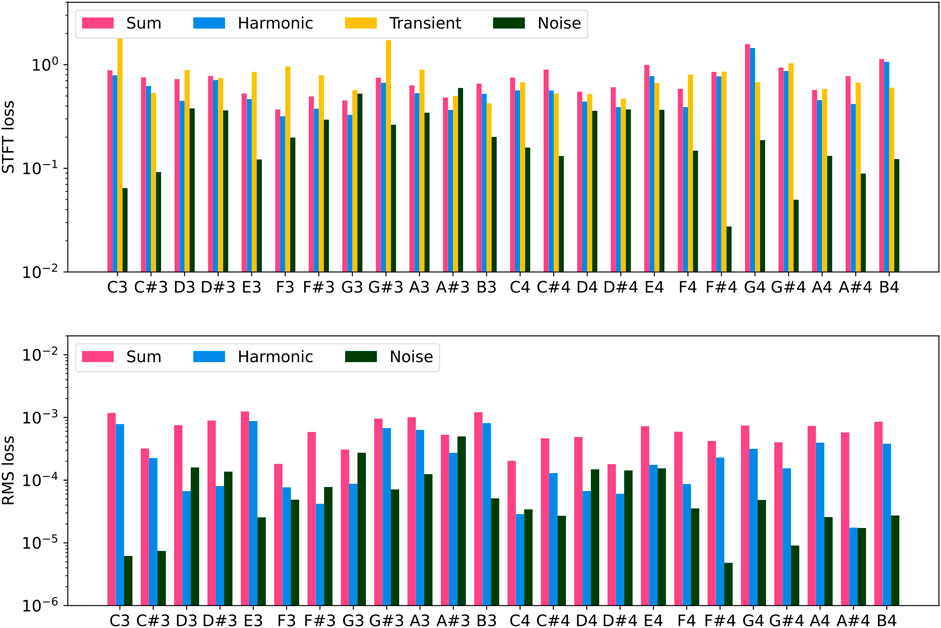
Figure 7. STFT (top) and RMS (bottom) losses of the test set across all the keys and considering the upright piano. STFT losses are normalized by the norm of the target spectrogram, as in the training process, and the window resolutions employed are identical to those used for the STFT of the quasi-harmonic component. The y-axis is on a logarithmic scale. Magenta bars refer to the sum of all components; blue bars refer to the quasi-harmonic component; the yellow bars refer to the transient component, and the dark green refer to the noise component.
The Cent losses, as reported in Figure 8, indicates a good match for inharmonicity for the quasi-harmonic module, reporting a maximum cent deviation of approximately
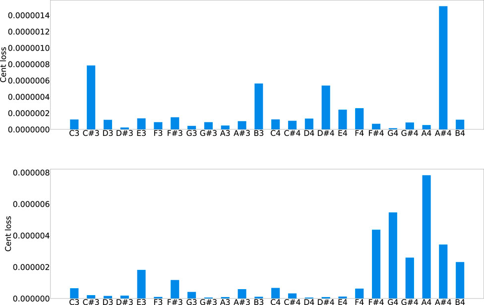
Figure 8. Cent loss for all the keys of the upright piano (top) and grand piano (bottom).
Figure 9 shows the results for the transient and noise components of an example note in the test set, corresponding to
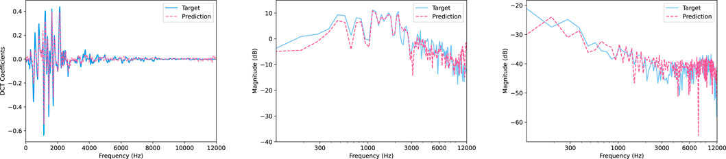
Figure 9. Predictions and targets for the
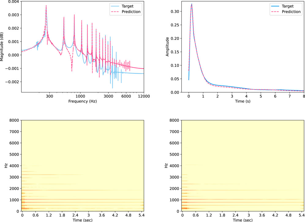
Figure 10. Predictions and targets for the
Table 1 reports the losses for the trichord scenarios. The measure indicates a good similarity between the prediction and the target, which is confirmed by the spectrograms of a trichord example in the test set: the
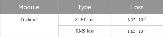
Table 1. Test set losses for the trichord dataset.
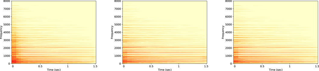
Figure 11. Spectrogram of the
A total of 20 participants took part in the MUSHRA test, consisting of 13 men and 7 women, aged between 26 and 36. All participants were trained musicians with varying levels of expertise, ranging from intermediate to expert. None reported any hearing impairment, and none met the criteria for exclusion due to clear and obvious rating errors. Figure 12 presents the results of the test, where the box plots illustrate the median, lower, and upper quartiles, as well as the maximum, minimum values, and outliers of the responses. It is evident that the sound generated by the model is perceptually distinguishable from that of a real piano, which was used to train the model, but the difference is not substantial. For the chords, the model provides a better sound than the simple sum of the individual notes, typical of most synthesis approaches. Table 2 presents a statistical analysis of the results based on the non-parametric Friedman test and Cliff’s delta. The results show small
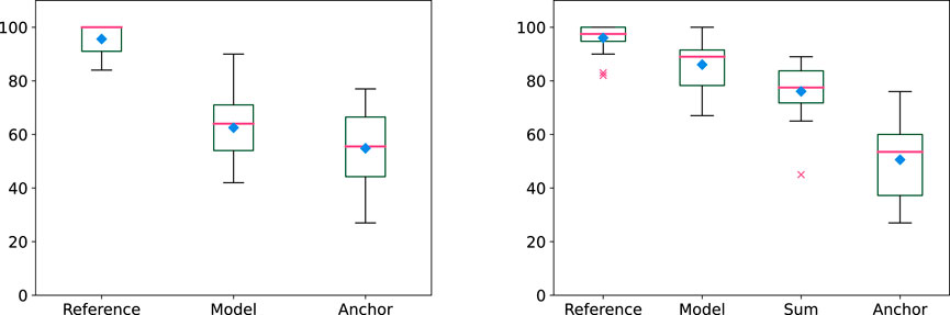
Figure 12. Box plot showing the rating results of the listening tests for single notes (left) and trichords (right). The magenta horizontal lines and the diamond markers indicate the median and the mean values, respectively. Outliers are displayed as crosses.
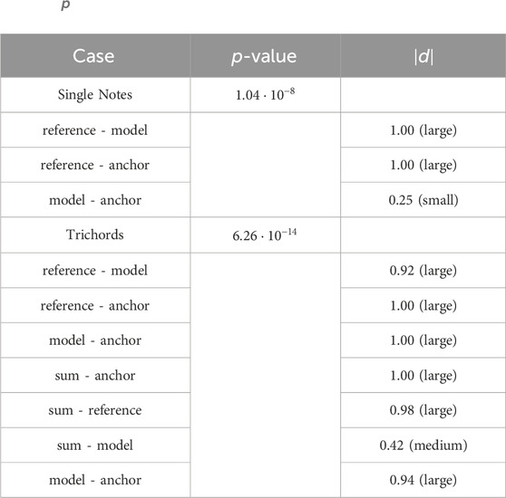
Table 2.
Figure 13 reports the related LDA projections for the single notes and trichords. In the first case, the comparison focuses on the sound variation at different velocities, while the second considers the difference between the sum and the actual trichord. The examples used from the models are included in the test set. We can see how, for single notes, the models’ predictions are confined in the same cluster of the acoustic piano, while the samples-based and physics-based digital piano examples are in different visible clusters. This suggests that the proposed methodology is able to simulate the sound changes due to different velocities. On the other hand, the trichords case shows that the acoustic cluster is separated from the model’s one, although the model cluster does not overlap with samples-based and physics-based clusters, which in this case are totally overlapped. Therefore, although the model behaves differently from the samples-based and physics models, whose emulations are close to the simple sum, it presents differences in the frequency components with respect to the acoustic case.
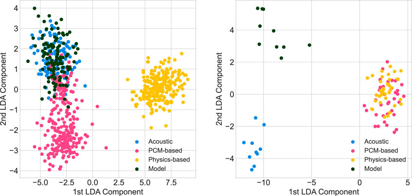
Figure 13. Projected feature vectors to 2D space using LDA for the case of single-note stimuli (left) and trichords (right).
4.1 Efficiency
Generating the damping parameters based on physical laws helps to restrict the layer sizes and, consequently, reduces the computational cost. Furthermore, utilizing target information such as the inharmonicity factor to initialize the training simplifies the learning challenges for the model, further contributing to the achievement of accuracy with smaller neural networks. The quasi-harmonic module comprises only 7,601 trainable parameters and requires
5 Discussion and conclusion
The paper presented a novel method to approach differentiable spectral modeling. The target sound, in this case, piano notes, is decomposed into quasi-harmonic, transient, and noise components. The harmonic part is synthesized using sinusoidal modeling and physics knowledge. From MIDI information, the trained model predicts the inharmonicity factor, the frequency-dependent damping coefficients, and the attack time. The inharmonicity factor and the frequency-dependent damping coefficients are computed using physical equations. A sine generator computes the partials multiplied by the amplitude envelope to generate the quasi-harmonic content. Beatings, double decay, and even phantom partials are included in the model, generating other sets of partials. The noise is targeted by predicting a time-varying filter to filter the white noise, its mean, and amplitude envelope across time. Finally, the transient component is generated using a deep convolutional oscillator that produces the discrete cosine transform (DCT) of the transient, which is later reversed. The network generating the DCT consists of a stack of upsampling and convolutional layers that generate a waveform from the MIDI information. The model is trained to emulate a specific piano by learning directly from actual sound recordings and analytical information extracted from them. Eventual imprecision in the analysis algorithms, physics-derived equations, or unconsidered physical aspects can negatively impact the resulting model’s accuracy. For example, at this stage, the soundboard influence is implicitly learned from the damping layer, and the room reverb is not included. The model learns three components separately, lowering the task’s complexity. The physical law guiding the generation of the quasi-harmonic content also helps lower the computational cost requirements. The architecture is designed to generate an arbitrary number of samples per inference iteration, thereby allowing flexibility and minimizing input-to-output latency. For this specific configuration, we have demonstrated the integration of more complex aspects, such as the coupling effect when different keys are struck simultaneously in trichords.
All three sub-models can provide overall good emulation accuracy. The quasi-harmonic content matches the partial placements, although it becomes less precise at higher partial. Frequently, these are predicted to have a greater energy than the target piano recordings. The RMS envelopes show a good matching as well, and the predicted signal presents two decay rates. Also, the generation of the transient and noisy parts presents overall spectral accuracy. On the other hand, listening tests still underscore perceptual differences between the target and emulated piano sounds. In particular, the attack portion of the note is where most inaccuracies appear to be concentrated. This is evident when listening to the audio examples we have made publicly available, and it was also highlighted during informal post-test discussions with the majority of participants.
The computational bottleneck of the model is represented by the transient generation that requires a relatively large neural network. The discrete cosine transform allows the restriction of the size of the vector to be generated since the limited extension of the frequency content and, in turn, lowers the network’s effort. Finally, the method relies on the quasi-harmonic, transient, and noise components separation quality, which is crucial for learning, and on the precision of the utilized physical laws. This aspect introduces further flexibility to the model. Once trained, the model accepts variations on its equation, and users can potentially navigate different equations, such as, in this case, the attack envelope and energy damping. The possibility of emulating the sound of individual piano notes without the requirements of storing audio samples can also be a memory-efficient alternative to the sample-based synthesizer. In the future, we will develop datasets to integrate other complex performance scenarios, such as re-stricken keys, arpeggios, and chords consisting of different numbers of notes and arbitrarily simultaneously played notes. Another aspect to further investigate is the inclusion of phase information in the quasi-harmonic model, which could potentially enhance the accuracy of note attack. In the current model, convergence issues arise and gradients tend to explode when phase information is incorporated—that is, when both the frequency and phase of each partial are predicted. The underlying reasons for this phenomenon remain unknown; however, they may lie in the cyclic nature of the phase.
Data availability statement
The datasets presented in this study can be found in online repositories. The names of the repository/repositories and accession number(s) can be found in the article/supplementary material.
Ethics statement
This research was conducted in accordance with the University of Oslo’s research ethics guidelines and the Norwegian Research Ethics Act, which stipulate that no clearance, approval, or notification to relevant bodies is necessary when research does not involve the collection or use of personal data, as is the case with the listening test described in this article. In line with the requirements of the Norwegian Agency for Shared Services in Education and Research, all participants were fully informed about the study and provided their written consent at its outset. The studies adhered to local legislation and institutional requirements, ensuring that participants’ consent was knowingly and voluntarily given.
Author contributions
RS: Conceptualization, Data curation, Investigation, Methodology, Writing–original draft. SF: Supervision, Writing–review and editing.
Funding
The author(s) declare that no financial support was received for the research, authorship, and/or publication of this article.
Conflict of interest
The authors declare that the research was conducted in the absence of any commercial or financial relationships that could be construed as a potential conflict of interest.
Publisher’s note
All claims expressed in this article are solely those of the authors and do not necessarily represent those of their affiliated organizations, or those of the publisher, the editors and the reviewers. Any product that may be evaluated in this article, or claim that may be made by its manufacturer, is not guaranteed or endorsed by the publisher.
Footnotes
1https://zenodo.org/records/2573232
2https://github.com/RiccardoVib/STN_Neural
References
Bank, B., and Sujbert, L. (2003). “Modeling the longitudinal vibration of piano strings,” in Proc. Stockholm Music acoust (Stockholm, Sweden: Conf.), 143–146.
Bank, B., and Sujbert, L. (2005). Generation of longitudinal vibrations in piano strings: from physics to sound synthesis. J. Acoust. Soc. Am. 117, 2268–2278. doi:10.1121/1.1868212
Birnbaum, S., Kuleshov, V., Enam, Z., Koh, P. W. W., and Ermon, S. (2019). Temporal film: capturing long-range sequence dependencies with feature-wise modulations. Adv. Neural Inf. Process. Syst. 32.
Caspe, F., McPherson, A., and Sandler, M. (2022). Ddx7: differentiable fm synthesis of musical instrument sounds. arXiv Prepr. arXiv:2208.06169.
Chabassier, J., Chaigne, A., and Joly, P. (2014). Time domain simulation of a piano. part 1: model description. ESAIM Math. Model. Numer. Analysis 48, 1241–1278. doi:10.1051/m2an/2013136
Cuesta, C., and Valette, C. (1988). Evolution temporelle de la vibration des cordes de clavecin. Acta Acustica united Acustica 66, 37–45.
Conklin Jr, H. A. (1999). Generation of partials due to nonlinear mixing in a stringed instrument. J. Acoust. Soc. Am. 105, 536–545. doi:10.1121/1.424589
Dauphin, Y. N., Fan, A., Auli, M., and Grangier, D. (2017). “Language modeling with gated convolutional networks,” in International conference on machine learning (Sydney, Australia: PMLR), 933–941.
Driedger, J., Müller, M., and Disch, S. (2014). “Extending harmonic-percussive separation of audio signals,” in Ismir.
Ege, K. (2009). La table d’harmonie du piano-Études modales en basses et moyennes fréquences. Paris, France: Ecole Polytechnique X. Ph.D. thesis.
Engel, J., Hantrakul, L., Gu, C., and Roberts, A. (2020). Ddsp: differentiable digital signal processing. Int. Conf. Learn. Represent. doi:10.1109/LSP.2018.2880284
Etchenique, N., Collin, S. R., and Moore, T. R. (2015). Coupling of transverse and longitudinal waves in piano strings. J. Acoust. Soc. Am. 137, 1766–1771. doi:10.1121/1.4916708
Hawthorne, C., Stasyuk, A., Roberts, A., Simon, I., Huang, C. A., Dieleman, S., et al. (2019). Enabling factorized piano music modeling and generation with the maestro dataset. Int. Conf. Learn. Represent.
Issanchou, C., Bilbao, S., Le Carrou, J., Touzé, C., and Doaré, O. (2017). A modal-based approach to the nonlinear vibration of strings against a unilateral obstacle: simulations and experiments in the pointwise case. J. Sound. Vibr. 393, 229–251. doi:10.1016/j.jsv.2016.12.025
ITU-R (2015). Bs.1534-3, method for the subjective assessment of intermediate quality level of audio systems. Geneva, Switzerland: International Telecommunication Union.
Jonason, N., Wang, X., Cooper, E., Juvela, L., Sturm, B. L., and Yamagishi, J. (2023). Ddsp-based neural waveform synthesis of polyphonic guitar performance from string-wise midi input. arXiv Prepr. arXiv:2309.07658.
Kawamura, M., Nakamura, T., Kitamura, D., Saruwatari, H., Takahashi, Y., and Kondo, K. (2022). “Differentiable digital signal processing mixture model for synthesis parameter extraction from mixture of harmonic sounds,” in Ieee int. Conf. On acoustics, speech and signal processing (ICASSP).
Kingma, D. P., and Ba, J. (2014). Adam: a method for stochastic optimization. Int. Conf. Learn. Represent.
Kreković, G. (2022). “Deep convolutional oscillator: synthesizing waveforms from timbral descriptors,” in Proceedings of the international conference on sound and music computing (SMC), 200–206.
Liu, Y., Jin, C., and Gunawan, D. (2023). Ddsp-sfx: acoustically-guided sound effects generation with differentiable digital signal processing. In Proc. of the Conf. Digital Audio Effects (DAFx)
Mezza, A. I., Giampiccolo, R., De Sena, E., and Bernardini, A. (2024). Data-driven room acoustic modeling via differentiable feedback delay networks with learnable delay lines. EURASIP J. Audio, Speech, Music Process. 2024, 51. doi:10.1186/s13636-024-00371-5
Pascanu, R., Mikolov, T., and Bengio, Y. (2013). “On the difficulty of training recurrent neural networks,” in Int. Conf. on machine learning.
Podlesak, M., and Lee, A. R. (1988). Dispersion of waves in piano strings. J. Acoust. Soc. Am. 83, 305–317. doi:10.1121/1.396432
Renault, L., Mignot, R., and Roebel, A. (2022). “Differentiable piano model for midi-to-audio performance synthesis,” in Proc. Of the conf. On digital audio effects (DAFx).
Schoeffler, M., Bartoschek, S., Stöter, F., Roess, M., Westphal, S., Edler, B., et al. (2018). webmushra—a comprehensive framework for web-based listening tests. J. Open Res. Softw. 6 (8), 8. doi:10.5334/jors.187
Serra, X., and Smith, J. (1990). Spectral modeling synthesis: a sound analysis/synthesis system based on a deterministic plus stochastic decomposition. Comput. Music J. 14, 12–24. doi:10.2307/3680788
Shan, S., Hantrakul, L., Chen, J., Avent, M., and Trevelyan, D. (2022). “Differentiable wavetable synthesis,” in Ieee int. Conf. On acoustics, speech and signal processing (ICASSP).
Shier, J., Caspe, F., Robertson, A., Sandler, M., Saitis, C., and McPherson, A. (2023). Differentiable modelling of percussive audio with transient and spectral synthesis. Forum Acusticum.
Simionato, R., and Fasciani, S. (2023). “A comparative computational approach to piano modeling analysis,” in Proceedings of the international conference on sound and music computing (SMC).
Simionato, R., Fasciani, S., and Holm, S. (2024). Physics-informed differentiable method for piano modeling. Front. Signal Process. 3, 1276748. doi:10.3389/frsip.2023.1276748
Tan, J. J. (2017). Piano acoustics: string’s double polarisation and piano source identification. Paris, France: Université Paris Saclay (COmUE). Ph.D. thesis.
Verma, T. S., and Meng, T. H. (2000). Extending spectral modeling synthesis with transient modeling synthesis. Comput. Music J. 24, 47–59. doi:10.1162/014892600559317
Weinreich, G. (1977). Coupled piano strings. J. Acoust. Soc. Am. 62, 1474–1484. doi:10.1121/1.381677
Keywords: sound source modeling, physics-informed modeling, acoustic modeling, deep learning, piano synthesis, differentiable digital signal processing
Citation: Simionato R and Fasciani S (2025) Sines, transient, noise neural modeling of piano notes. Front. Signal Process. 4:1494864. doi: 10.3389/frsip.2024.1494864
Received: 11 September 2024; Accepted: 30 December 2024;
Published: 29 January 2025.
Edited by:
Farook Sattar, University of Victoria, CanadaReviewed by:
Tim Ziemer, University of Hamburg, GermanyJelena Ćertić, University of Belgrade, Serbia
Copyright © 2025 Simionato and Fasciani. This is an open-access article distributed under the terms of the Creative Commons Attribution License (CC BY). The use, distribution or reproduction in other forums is permitted, provided the original author(s) and the copyright owner(s) are credited and that the original publication in this journal is cited, in accordance with accepted academic practice. No use, distribution or reproduction is permitted which does not comply with these terms.
*Correspondence: Riccardo Simionato, cmljY2FyZG8uc2ltaW9uYXRvQGltdi51aW8ubm8=