State-space estimation of spatially dynamic room impulse responses using a room acoustic model-based prior

Room impulse responses (RIRs) between static loudspeaker and microphone locations can be estimated using a number of well-established measurement and inference procedures. While these procedures assume a time-invariant acoustic system, time variations need to be considered for the case of spatially dynamic scenarios where loudspeakers and microphones are subject to movement. If the RIR is modeled using image sources, then movement implies that the distance to each image source varies over time, making the estimation of the spatially dynamic RIR particularly challenging. In this paper, we propose a procedure to estimate the early part of the spatially dynamic RIR between a stationary source and a microphone moving on a linear trajectory at constant velocity. The procedure is built upon a state-space model, where the state to be estimated represents the early RIR, the observation corresponds to a microphone recording in a spatially dynamic scenario, and time-varying distances to the image sources are incorporated into the state transition matrix obtained from static RIRs at the start and end points of the trajectory. The performance of the proposed approach is evaluated against state-of-the-art RIR interpolation and state-space estimation methods using simulations, demonstrating the potential of the proposed state-space model.

1 Introduction

A room impulse response (RIR) is the time-domain representation of the linear time-invariant (LTI) system that uniquely characterizes the cumulative impact of a room on sound waves between a specific static source and a microphone’s position, effectively representing the room’s acoustic environment. This concept is fundamental to various acoustic signal processing applications, including source localization (Evers et al., 2020), dereverberation (Naylor and Gaubitch, 2010), echo cancellation (Elko et al., 2003), and spatial audio reproduction (Schissler et al., 2017). Considerable research has been dedicated to developing robust measurement (Stan et al., 2002; Szöke et al., 2018) and estimation (Lin and Lee, 2006; Crocco and Bue, 2015; Ratnarajah et al., 2022) techniques for capturing RIRs, particularly in scenarios where the source and microphone remain static within the acoustic environment (Stan et al., 2002; Szöke et al., 2018). However, real-world situations often involve spatially dynamic scenarios, where sources and microphones are subject to movement. This paper addresses the challenge of accurately estimating the early part of RIRs along a trajectory in a time-varying acoustic scenario with a stationary source and a moving microphone. This can be thought of as a time-varying system identification problem where the system to be identified may be referred to as a time-variant RIR.

In this context, it is important to consider the apparent contradiction between the previously defined RIR as an LTI system representation and the concept of a time-variant RIR. In this paper, the acoustic environment itself is assumed to be time-invariant, in which case an RIR between two static positions indeed corresponds to an LTI system. RIRs, however, are inherently location-variant—they depend on the locations of the source and the microphone. The time-variant RIR, as considered here, can be defined as the time-varying system representation (Cherniakov, 2003) relating the source signal to the microphone signal if the microphone moves—that is, has a time-varying location. In discrete time, this time-variant RIR can also be thought of as a collection of RIRs in the LTI sense over different time-instances: the location of the microphone changes at each time step, leading to a new discrete position in space associated with a time-invariant RIR. Time-variant RIR estimation, as defined above, has relevance across numerous acoustic signal processing applications, especially amid the growing interest in virtual acoustic environments. For instance, Ajdler et al. (2007) demonstrated the use of time-varying acoustic system models for enabling the rapid measurement of head-related impulse responses. Moreover, sub-optimal estimations of time-variant RIRs can impair the effectiveness of echo-cancellation systems in telepresence and communication technologies (Nophut et al., 2024).

In order to contextualize our contribution in estimating the early part of a time-variant RIR, it is necessary to provide a brief outline of the related literature. In this context, the concept of spatial RIR interpolation is highly relevant given that we can consider a time-varying RIR as a collection of RIRs over a discrete set of locations. RIR interpolation facilitates sound field rendering for dynamic source–microphone positions by filling spatial gaps in RIR data, as measurements or simulations are usually limited to sparse grids. Numerous approaches have been proposed for RIR interpolation, including compressed sensing methods (Mignot et al., 2013; Katzberg et al., 2018), spherical harmonics (Borra et al., 2019), physics-based models (Antonello et al., 2017; Hahmann and Fernandez-Grande, 2022), directional RIRs (Zhao et al., 2022), and neural networks (Pezzoli et al., 2022; Karakonstantis et al., 2024). Haneda et al. (1999) introduced a frequency-domain approach for interpolating room transfer functions (RTFs), which is particularly effective at lower frequencies; it was extended by Das et al. (2021). Additionally, several techniques for the interpolation of head-related transfer functions (HRTFs), which are critical for accurate binaural rendering and share some methodological approaches with RTF interpolation, have been explored (Carty, 2010). For the purpose of this paper, we focus on the interpolation of an RIR at a point between two microphone locations given their estimated RIRs for a common stationary source. Kearney et al. (2009) introduced Dynamic Time Warping (DTW)-based interpolation, dividing RIRs into early reflections and diffuse decay. This method temporally aligns and linearly interpolates early reflections while modeling the tail using the approach of Masterson et al. (2009) and laying the foundation for subsequent developments. Garcia-Gomez and Lopez (2018) expanded on Kearney’s work, enhancing algorithm robustness and computational efficiency while retaining the core interpolation technique. Building on this, Bruschi et al. (2020) refined peak finding and matching aspects of the interpolation technique. Geldert et al. (2023) proposed a novel approach using partial optimal transport for interpolation, enabling non-bijective mapping of sound events between the early part of RIRs. It is important to highlight that these interpolation approaches operate outside of a conventional system identification framework. Instead, they use a limited set of measured RIRs and predominantly rely on a room acoustic sound propagation model such as the image source method (ISM) (Allen and Berkley, 1979). As opposed to interpolation strategies, fully data-driven approaches for estimating time-variant RIRs have also been investigated. In this case, the estimation relies directly on the source and microphone signals and can be framed as a system identification or adaptive filtering problem. This approach has been largely motivated by the need to obtain rapid measurements of head-related impulse responses (Enzner, 2008; Hahn and Spors, 2015) and for echo cancellation (Antweiler and Symanzik, 1995; Enzner, 2010), where a typical scenario involves an excitation signal being continuously captured by a moving microphone. Using carefully designed excitation signals (Hahn and Spors, 2015; Kuhl et al., 2018), time-variant RIRs can be estimated using a normalized least mean squares (NLMS) algorithm (Enzner, 2008; Antweiler et al., 2012) or more generally using a Kalman filter (Enzner, 2010). In the context of this paper, a Kalman filter is of particular interest as it is derived from a state-space model of the dynamic system where the state to be estimated is the time-variant RIR (Enzner, 2010). In such a state-space model, the evolution of the time-variant RIR is explicitly modeled using a first-order difference equation, which allows more modeling flexibility than other adaptive algorithms such as NLMS. One popular choice for the first-order difference model is to relate the states at two time instants by a transition factor and an additional process noise term. The transition coefficient and process noise covariance are typically set according to the expected variability of the state, influencing the convergence behavior of the Kalman filter. For instance, in Nophut et al. (2024), the transition coefficient was modeled as a function of the microphone velocity.

We here consider the problem of estimating the early part of the time-variant RIR between a stationary source and a microphone moving on a linear trajectory at constant velocity. We propose integrating RIR interpolation, derived from a room acoustic model, into a state-space-based framework for RIR estimation, thereby merging data-driven approaches with physical modeling. More specifically, rather than relying solely on a state transition factor within the state equation, we propose incorporating the ISM into a state transition matrix between the early segments of consecutive RIRs. We derive an analytical model for this transition matrix and subsequently propose estimating it from static RIRs at the trajectory’s start and end points using a DTW-based algorithm. The proposed approach's performance is evaluated through simulations by comparing it to two alternatives: one that relies solely on the state equation for RIR estimation, resembling a pure interpolation method with the ISM-based transition matrix, and another that uses a conventional state-space estimation with a simple state transition factor. Our findings suggest that the proposed state-space model outperforms both alternatives in terms of normalized misalignment between the simulated “ground-truth” RIRs and estimated RIRs.

The subsequent sections of this paper are organized as follows. Section 2 introduces the signal model and provides an overview of the most pertinent state-of-the-art methods. Section 3 elaborates on the proposed RIR state-space model and outlines the update equations of the Kalman filter used to recursively estimate the defined state. Section 4 offers detailed derivations of the proposed room acoustic model-based state transition matrix. Finally, Section 5 presents experimental validation through simulations, followed by a discussion of the results.

2 Signal model, problem statement, and related state of the art

2.1 Signal model and problem statement

We first introduce the signal model to formally define the concept of an RIR as employed in this paper. When we henceforth use the term “RIR”, it will specifically pertain to the early part of the RIRs, as we do not address the estimation of the late reverberant tail. We also assume that the source location remains static. Let $k$ denote the time index, and let the location of the microphone relative to the linear trajectory be denoted by the one-dimensional location index $l$. If the microphone location is time-variant, an RIR defines the LTI system relating a source signal $x(k)$ to an observed signal $y(l,k)$. Let the RIR for microphone location $l$ be denoted by $h(l,n)$, where $n$ indexes the time-shift of the RIR samples. The signals $x(k)$ and $y(l,k)$ are then related by

$y\left(l,k\right)={\displaystyle \sum _{n=0}^{N-1}}h\left(l,n\right)x\left(k-n\right)+v\left(k\right),(1)$

where $v(k)$ is a noise term that we generally assume to be present in the observed signal and may include late reverberation. Now, defining the vectors $\mathbf{x}(k)$ and $\mathbf{h}(l)$ as

$\mathbf{x}\left(k\right)={\left(\begin{array}{cccc}\hfill x\left(k\right)\hfill & \hfill x\left(k-1\right)\hfill & \hfill \dots \hfill & \hfill x\left(k-N+1\right)\hfill \end{array}\right)}^T,(2)$

$\mathbf{h}\left(l\right)={\left(\begin{array}{cccc}\hfill h\left(l,0\right)\hfill & \hfill h\left(l,1\right)\hfill & \hfill \dots \hfill & \hfill h\left(l,N-1\right)\hfill \end{array}\right)}^T,(3)$

the convolution in Equation 1 can alternatively be written as

$y\left(l,k\right)={\mathbf{x}}^T\left(k\right)\mathbf{h}\left(l\right)+v\left(k\right).(4)$

Within the scope of this paper, we assume a linear microphone trajectory of length $d$, divided into $L$ equidistant locations spaced by $\mathrm{\Delta }d$ and indexed as $l=0,\dots ,L-1$, as illustrated in Figure 1, such that $L=d/\mathrm{\Delta }d+1$. We consider the problem of estimating $\mathbf{h}(l)$ using the source signal $x(k)$ and the observed signal $y(l,k)$ if the microphone moves along the trajectory at a constant velocity ${\mu }_{\text{rx}}$—that is, if $l$ varies over time. For this, we make the assumptions that $\mathbf{h}(0)$ and $\mathbf{h}(L-1)$ are known, and that the time intervals which the individual reflections occupy within the time-variant RIR over the range of the trajectory do not overlap. An example of $\mathbf{h}(0)$ and $\mathbf{h}(L-1)$ including only first-order reflections is shown in Figure 2, where peaks corresponding to the same source or reflection are labeled by the same number in each RIR.

Figure 1

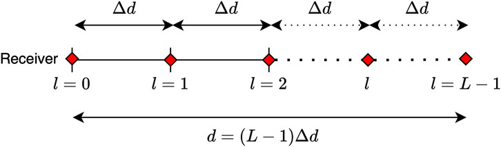
Figure 1. Linear microphone trajectory of length $d$ divided into $L$ equidistant locations spaced by $\mathrm{\Delta }d$ and indexed as $l=0,\dots ,L-1$ such that $d=(L-1)\mathrm{\Delta }d$.

Figure 2

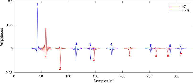
Figure 2. An example of simulated RIRs, $\mathbf{h}(0)$ and $\mathbf{h}(L-1)$, including only first-order reflections. Peaks corresponding to the same source or reflection are labeled by the same number in each RIR.

2.2 Related state of the art

Before introducing the proposed approach, it is instructive to briefly introduce the most relevant concepts used in the state of the art. On the one hand, we consider RIR interpolation approaches that estimate $\mathbf{h}(l)$ from $\mathbf{h}(0)$ and $\mathbf{h}(L-1)$ only based on a room acoustic sound propagation model, without making use of an observed signal $y(l,k)$. On the other hand, we consider data-driven approaches that estimate $\mathbf{h}(l)$ in an adaptive manner from a data set containing $x(k)$ and $y(l,k)$ over multiple time indexes $k$ for a moving microphone, but without exploiting a room acoustic sound propagation model.

As previously mentioned, some RIR interpolation approaches (Kearney et al., 2009; Geldert et al., 2023) are motivated by the ISM for room acoustic sound propagation, which expresses an RIR as a sum of contributions from the original source and so-called image sources representing reflections from the boundaries of the room. Based on this model, RIR interpolation approaches infer the location-variant time of arrival (TOA) as well as the amplitude of the direct component and individual reflections (or equivalently, source and image source components) at a particular location $l$ using the RIRs $\mathbf{h}(0)$ and $\mathbf{h}(L-1)$. The general principle can be described as follows. Assuming that reflections corresponding to the same image source in $\mathbf{h}(0)$ and $\mathbf{h}(L-1)$ can be identified, let ${\mathbf{n}}_r(0)$ and ${\mathbf{n}}_r(L-1)$ be vectors collecting the respective time-shift indices of the direct component and these reflections in $\mathbf{h}(0)$ and $\mathbf{h}(L-1)$. The corresponding time-shift indices of $\mathbf{h}(l)$ can be interpolated as

${\mathbf{n}}_r\left(l\right)={\mathbf{n}}_r\left(0\right)+\mathrm{r}\mathrm{o}\mathrm{u}\mathrm{n}\mathrm{d}\left(\beta \left(l\right)\left({\mathbf{n}}_r\left(L-1\right)-{\mathbf{n}}_r\left(0\right)\right)\right),(5)$

where ${\mathbf{n}}_r(L-1)-{\mathbf{n}}_r(0)$ can be conceived as sample-based time differences of arrival (TDOAs), $\beta (l)\in [\mathrm{0,1}]$ with $\beta (0)=0$ and $\beta (L-1)=1$, and $\mathrm{r}\mathrm{o}\mathrm{u}\mathrm{n}\mathrm{d}(\cdot )$ defines a rounding operation. The function $\beta (l)$ can be defined such that the interpolation is correct for the direct component (Kearney et al., 2009). Applying a similar interpolation rule for the amplitudes of the direct component and reflections, an estimate of $\mathbf{h}(l)$ can then be obtained. The collections of corresponding indices ${\mathbf{n}}_r(0)$ and ${\mathbf{n}}_r(L-1)$ can, for instance, be found by means of Dynamic Time Warping with $\mathbf{h}(0)$ and $\mathbf{h}(L-1)$ as inputs (Kearney et al., 2009; Bruschi et al., 2020). Here, an accurate identification of all corresponding reflections requires that their order of arrival is the same in $\mathbf{h}(0)$ and $\mathbf{h}(L-1)$.

Data-driven approaches (Enzner, 2010) to the estimation of location- or time-variant RIRs do not rely on explicit modeling of room acoustic sound propagation, but instead perform adaptive system identification given a data set containing $x(k)$ and $y(l,k)$ over multiple time indexes $k$. For the moment, let us assume that the moving microphone crosses one location $l$ at each time instant $k$, such that the location-variant RIR $\mathbf{h}(l)$ can equivalently be thought of as a time-variant RIR $\mathbf{h}(k)$ with $k=l$. The convolution in Equation 1 then becomes

$y\left(k\right)={\displaystyle \sum _{n=0}^{N-1}}h\left(k,n\right)x\left(k-n\right)+v\left(k\right).(6)$

This can be expressed similarly to Equation 4 using the definitions in Equations 2 and 3. A popular approach to adaptively estimate $\mathbf{h}(k)$ is the Kalman filter, whose update equations are obtained from a state-space model where $\mathbf{h}(k)$ is the state. A commonly used state-space model can be defined as

$\mathbf{h}\left(k\right)=\alpha \mathbf{h}\left(k-1\right)+\mathbf{w}\left(k\right),(7)$

$y\left(k\right)={\mathbf{x}}^T\left(k\right)\mathbf{h}\left(k\right)+v\left(k\right),(8)$

where the state equation in Equation 7 models the evolution of the state as a first-order difference equation, and the observation equation (Equation 8) relates the state to the observation $y(k)$ and is identical to Equation 6. The model commonly chosen in Equation 7 defines a factor $\alpha$, referred to as the “forgetting” or “transition” factor, and a noise term $\mathbf{w}(k)$, referred to as “process noise”, for which the covariance matrix is required in the Kalman filter. In practice, the choice of $\alpha$ and the covariance matrix of $\mathbf{w}(k)$ is typically not directly motivated by a physical model of the RIR evolution. Instead, they are often considered tuning parameters that can be used to control the convergence behavior of the Kalman filter, although they can be tuned depending on physical parameters such as the velocity of the microphone (Nophut et al., 2024).

3 Proposed RIR state-space model

In the proposed approach, we aim to include prior knowledge on room acoustic sound propagation into a state-space model for time-variant RIR estimation. To this end, rather than resorting to a scalar factor as in Equation 7, we assume that the relation between two RIRs $\mathbf{h}(l)$ and $\mathbf{h}(l-1)$ on the trajectory can approximately be modeled by a location-invariant transition matrix $\mathbf{A}$ as

$\mathbf{h}\left(l\right)\approx \mathbf{A}\mathbf{h}\left(l-1\right)(9)$

for $l=1,\dots ,L-1$. The transition matrix $\mathbf{A}$ will be used to model changes in the TOA of the direct component and the early reflections between the neighboring locations $l$ and $l-1$ and will be applied in the state equation of the proposed state-space model. As described in Section 4, the analytical definition of $\mathbf{A}$ will be based on the ISM, which also serves as the foundation of the RIR interpolation approaches discussed in Section 2.2. Furthermore, we will show that the transition matrix $\mathbf{A}$ can be modeled as location-invariant if the time intervals which the individual reflections occupy in the time-variant RIR over the range of the trajectory do not overlap, which is also implicitly assumed in Kearney et al. (2009) and Geldert et al. (2023). In practice, an estimate of $\mathbf{A}$ can be obtained from the presumed knowledge of the RIRs $\mathbf{h}(0)$ and $\mathbf{h}(L-1)$ at the start and the end of the trajectory, as will be discussed in Section 4.3.

While it is possible to interpolate between $\mathbf{h}(0)$ and $\mathbf{h}(L-1)$ based on $\mathbf{A}$ only as $\mathbf{h}(l)\approx {\mathbf{A}}^l\mathbf{h}(0)$, a more accurate estimate can be obtained by using the signals recorded along the trajectory with a microphone moving at a constant velocity. Without loss of generality, let $k=0$ denote the start of the recording at location $l=0$. For a given velocity ${\mu }_{\text{rx}}$ of the microphone and temporal sampling period $T_s$, the smallest possible spatial period $\mathrm{\Delta }d$ that could be used is given by ${\mu }_{\text{rx}}{T}_s$. In this case, one RIR estimate can be obtained per time sample. In the proposed approach, we also consider spatial periods of

$\mathrm{\Delta }d=\mathrm{\Omega }{\mu }_{\text{rx}}{T}_s,$

where $\mathrm{\Omega }$ is a positive integer that can be understood as a spatial down-sampling factor. If the microphone is at location with index $l$, we then observe sample

$k=l\mathrm{\Omega }.$

With Equation 9 and defining $y_{\mathrm{\Omega }}(l)=y(l\mathrm{\Omega })$, ${\mathbf{x}}_{\mathrm{\Omega }}(l)=\mathbf{x}(l\mathrm{\Omega })$, and $v_{\mathrm{\Omega }}(l)=v(l\mathrm{\Omega })$ for ease of presentation, we can define the state-space model of the proposed approach as

$\mathbf{h}(l)=\mathbf{A}\mathbf{h}(l-1)+\mathbf{w}(l),(10)$

$y_{\mathrm{\Omega }}(l)={\mathbf{x}}_{\mathrm{\Omega }}^T(l)\mathbf{h}(l)+v_{\mathrm{\Omega }}(l),(11)$

where $\mathbf{w}(l)$ is the process noise accounting for modeling errors in the definition of $\mathbf{A}$. From the state-space model, an estimate $\widehat{\mathbf{h}}(l)$ of $\mathbf{h}(l)$ can be obtained using the Kalman filter with one recursion per location $l$. The Kalman filter update equations are outlined in the next section.

3.1 Update equations of the Kalman filter

The Kalman filter (Simon, 2006) can be used to recursively estimate the state defined by a state-space model. For the proposed state-space model in Equations 10 and 11, let $\mathbf{Q}=\mathrm{E}[\mathbf{w}(l){\mathbf{w}}^T(l)]$ and $R=\mathrm{E}[v_{\mathrm{\Omega }}^2(l)]$ be the presumed location-invariant covariance matrix of $\mathbf{w}(l)$ and variance of $v_{\mathrm{\Omega }}(l)$, respectively, where $\mathrm{E}[\cdot ]$ denotes the expectation operation. The update equations of the Kalman filter for the model in Equations 10 and 11 are then given by

$\widehat{\mathbf{h}}\left(l\right)=\mathbf{A}{\widehat{\mathbf{h}}}^{+}\left(l-1\right),.(12)$

$\mathbf{P}\left(l\right)=\mathbf{A}{\mathbf{P}}^{+}\left(l-1\right){\mathbf{A}}^T+\mathbf{Q},.(13)$

$\mathbf{k}\left(l\right)=\frac{\mathbf{P}\left(l\right){\mathbf{x}}_{\mathrm{\Omega }}\left(l\right)}{{\mathbf{x}}_{\mathrm{\Omega }}^T\left(l\right)\mathbf{P}\left(l\right){\mathbf{x}}_{\mathrm{\Omega }}\left(l\right)+R},(14)$

${\widehat{\mathbf{h}}}^{+}\left(l\right)=\widehat{\mathbf{h}}\left(l\right)+\mathbf{k}\left(l\right)\left(y_{\mathrm{\Omega }}\left(l\right)-{\mathbf{x}}_{\mathrm{\Omega }}^T\left(l\right)\widehat{\mathbf{h}}\left(l\right)\right),.(15)$

${\mathbf{P}}^{+}\left(l\right)=\left(\mathbf{I}-\mathbf{k}\left(l\right){\mathbf{x}}_{\mathrm{\Omega }}^T\left(l\right)\right)\mathbf{P}\left(l\right),(16)$

where Equations 12 and 13 are commonly referred to as the prediction step producing prior estimates, and Equations 14–16 are referred to as the update step producing posterior estimates. In these equations, $\widehat{\mathbf{h}}(l)$ and ${\widehat{\mathbf{h}}}^{+}(l)$ are state estimates, $\mathbf{P}(l)$ and ${\mathbf{P}}^{+}(l)$ are estimates of the state-estimation error covariance matrix, $\mathbf{k}(l)$ is the Kalman gain, $\mathbf{I}$ the identity matrix, and the superscript ⁺ distinguishes posterior from prior estimates. In the prediction step Equations 12 and 13, the previously acquired posterior estimates ${\widehat{\mathbf{h}}}^{+}(l-1)$ and ${\mathbf{P}}^{+}(l-1)$ are propagated based on the state Equation 10 only, without taking into account the observation at recursion $l$, yielding the prior estimates $\widehat{\mathbf{h}}(l)$ and $\mathbf{P}(l)$. The update step Equations 14–16 is based on the observation Equation 11. Here, the Kalman gain $\mathbf{k}(l)$ and the error term $y_{\mathrm{\Omega }}(l)-{\mathbf{x}}_{\mathrm{\Omega }}^T(l)\widehat{\mathbf{h}}(l)$ are computed based on $y_{\mathrm{\Omega }}(l)$ and ${\mathbf{x}}_{\mathrm{\Omega }}(l)$ and are used to update the prior estimates $\widehat{\mathbf{h}}(l)$ and $\mathbf{P}(l)$, yielding the posterior estimates ${\widehat{\mathbf{h}}}^{+}(l)$ and ${\mathbf{P}}^{+}(l)$.

To implement the Kalman filter, $\mathbf{Q}$ and $R$ are required as inputs. While $R$ can potentially be obtained from background noise recordings, $\mathbf{Q}$ can be considered a tuning parameter as the variance of $\mathbf{w}(l)=\mathbf{h}(l)-\mathbf{A}\mathbf{h}(l-1)$ will not be known exactly in practice. The Kalman filter also needs to be initialized by defining ${\widehat{\mathbf{h}}}^{+}(0)$ and ${\mathbf{P}}^{+}(0)$. As we assume that $\mathbf{h}(0)$ is known, we set ${\widehat{\mathbf{h}}}^{+}(0)=\mathbf{h}(0)$. This choice of ${\widehat{\mathbf{h}}}^{+}(0)$ corresponds to the assumption that the initial state estimation error is 0, such that ${\mathbf{P}}^{+}(0)$ can be chosen to have a small norm. Finally, a practical implementation requires an estimate of $\mathbf{A}$, which will be discussed in more detail in Sections 4.2 and 4.3.

At this point, it is instructive to interpret Equations 12–16 in relation to the state of the art as discussed in Section 2. In the interpolation approaches in Kearney et al. (2009) and Geldert et al. (2023) on the one hand, recorded signals are not available, which corresponds to the assumption that $y_{\mathrm{\Omega }}(l)=0$ and ${\mathbf{x}}_{\mathrm{\Omega }}(l)=0$. In this case, we find that ${\widehat{\mathbf{h}}}^{+}(l)=\widehat{\mathbf{h}}(l)$ and ${\mathbf{P}}^{+}(l)=\mathbf{P}(l)$ in Equations 15 and 16, i.e. $\widehat{\mathbf{h}}(l)$ no longer depends on $\mathbf{P}(l)$ and the Kalman filter update equations effectively reduce to $\widehat{\mathbf{h}}(l)=\mathbf{A}\widehat{\mathbf{h}}(l-1)={\mathbf{A}}^l\mathbf{h}(0)$. As $\mathbf{A}$ is defined by interpolating TOAs of reflections between $\mathbf{h}(0)$ and $\mathbf{h}(L-1)$ based on a room acoustic model, this case is conceptually similar to the aforementioned interpolation approaches and can be referred to as “linear interpolation.” The state-space space approaches in Enzner (2010), on the other hand, are obtained if $\mathrm{\Omega }=1$ and the state transition matrix $\mathbf{A}$ is replaced by a scalar $\alpha$.

4 Proposed room acoustic model-based transition matrix

This section provides a detailed explanation of the methodology followed to obtain a suitable room acoustic model-based transition matrix for use in Equation 10 and is organized as follows. In Section 4.1, we derive an analytical expression for a location-variant transition matrix model $\mathbf{A}(l)$ based on the ISM. A suitable modification of the analytical transition matrix for use in the state-space model is then proposed in Section 4.2 in order to obtain a location-invariant transition matrix model $\mathbf{A}$ valid within the limits of the trajectory. The models presented are parameterized by the exact reflection TOAs, which are not inherently available in practice. Therefore, Section 4.3 introduces an approach based on DTW to obtain an estimate of $\mathbf{A}$ from $\mathbf{h}(0)$ and $\mathbf{h}(L-1)$ by TDOA interpolation.

4.1 Analytical location-variant transition matrix model

The objective of this section is to derive a transition matrix model $\mathbf{A}(l)\in {\mathbb{R}}^{N\times N}$ that approximates the mapping between two RIRs $\mathbf{h}(l)$ and $\mathbf{h}(l-1)$:

$\mathbf{h}\left(l\right)\approx \mathbf{A}\left(l\right)\mathbf{h}\left(l-1\right).(17)$

An illustration of this relation along a given trajectory is shown in Figure 3A.

Figure 3

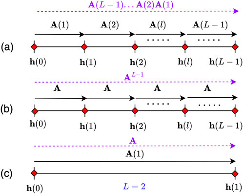
Figure 3. (A) Location-variant transition matrix model $\mathbf{A}(l)$ providing mapping between two RIRs $\mathbf{h}(l)$ and $\mathbf{h}(l-1)$ along a given trajectory. (B) Location-invariant transition matrix model $\mathbf{A}$ that approximates the mapping between two RIRs $\mathbf{h}(l)$ and $\mathbf{h}(l-1)$ along a given trajectory where the assumptions detailed in Section 4.2 hold. (C) Equivalent transition matrix models, $\mathbf{A}(1)$ and $\mathbf{A}$, for the special case of $L=2$—that is, a transition matrix between the start and end points of the trajectory.

To achieve this objective, we make use of the ISM. In this model, the RIR is expressed as the sum of contributions from the original sound source and additional image sources, which represent reflections within the room. Let the RIR at location $l$ with continuous time-shift $t$ be denoted by $h(l,t)$. With $\delta (t)$ denoting the Dirac delta function, the ISM models $h(l,t)$ as

$h\left(l,t\right)={\displaystyle \sum _{r\in \mathcal{R}}}{a}_r\left(l\right)\delta \left(t-{\tau }_r\left(l\right)\right),(18)$

where $r\in \mathcal{R}=\{\mathrm{0,1},..R-1\}$ is the (image) source or reflection index, and ${\tau }_r(l)$ and $a_r(l)$, respectively, denote the TOA and amplitude of the (image) source $r$ observed at location $l$. Ultimately, we aim to express a discretized version of $h(l,t)$ in terms of a discretized version of $h(l-1,t)$ as in Equation 17. To this end, we start by introducing parameters of $h(l-1,t)$ into $h(l,t)$ as follows.

$h\left(l,t\right)={\displaystyle \sum _{r\in \mathcal{R}}}{a}_r\left(l-1\right)\frac{a_r\left(l\right)}{a_r\left(l-1\right)}\delta \left(t-{\tau }_r\left(l\right)+{\tau }_r\left(l-1\right)-{\tau }_r\left(l-1\right)\right).(19)$

The inclusion of $a_r(l-1)/a_r(l-1)$ and ${\tau }_r(l-1)-{\tau }_r(l-1)$ preserves the definition of $h(l,t)$ in Equation 18, while allowing us to find a representation that more closely resembles $h(l-1,t)$. By incorporating ${\tau }_r(l-1)-{\tau }_r(l-1)$, we can isolate a Dirac delta function that only includes a time shift of ${\tau }_r(l-1)$ using the following identity derived from the sifting property (Hoskins, 2009):

$\delta \left(t-{\tau }_r\left(l\right)+{\tau }_r\left(l-1\right)-{\tau }_r\left(l-1\right)\right)={\int }_{-\infty }^{+\infty }\delta \left(t-{\tau }_r\left(l\right)+{\tau }_r\left(l-1\right)-t^{\prime }\right)\delta \left(t^{\prime }-{\tau }_r\left(l-1\right)\right)d{t}^{\prime }$

Therefore, Equation 19 can alternatively be expressed as

$h\left(l,t\right)={\displaystyle \sum _{r\in \mathcal{R}}}{\int }_{t^{\prime }}\frac{a_r\left(l\right)}{a_r\left(l-1\right)}\delta \left(t-{\tau }_r\left(l\right)+{\tau }_r\left(l-1\right)-t^{\prime }\right)a_r\left(l-1\right)\delta \left(t^{\prime }-{\tau }_r\left(l-1\right)\right)d{t}^{\prime }.(20)$

To obtain a discrete time-shift representation in terms of the time-shift index $n$, we impose a band limit with critical sampling period $T_s$. Band-limiting a Dirac delta function results in a sinc-function (Hoskins, 2009), which will be sampled at discrete time indices. Defining

${\mathrm{\Delta }}_r\left(l\right)={\tau }_r\left(l\right)-{\tau }_r\left(l-1\right)(21)$

as the TDOA of reflection $r$ between locations $l$ and $l-1$, we can now write Equation 23 as

$h\left(l,n\right)={\displaystyle \sum _{r\in \mathcal{R}}}{\displaystyle \sum _{n^{\prime }}}\frac{a_r\left(l\right)}{a_r\left(l-1\right)}\mathrm{s}\mathrm{i}\mathrm{n}\mathrm{c}\left(n-\frac{{\mathrm{\Delta }}_r\left(l\right)}{T_s}-n^{\prime }\right)a_r\left(l-1\right)\mathrm{s}\mathrm{i}\mathrm{n}\mathrm{c}\left(n^{\prime }-\frac{{\tau }_r\left(l-1\right)}{T_s}\right).(22)$

At this point, it is advantageous to introduce a time-shift-dependent approximation of Equation 22. At any $n$, the RIR sample $h(l,n)$ is dominated by a subset of reflections only, which we denote as $\tilde{\mathcal{R}}(l,n)$. Due to the decaying nature of the sinc-function, the product $\mathrm{s}\mathrm{i}\mathrm{n}\mathrm{c}\left(n-{\mathrm{\Delta }}_r(l)/T_s-n^{\prime }\right)\mathrm{s}\mathrm{i}\mathrm{n}\mathrm{c}\left(n^{\prime }-{\tau }_r(l-1)/T_s\right)$ in Equation 22 will have a prominent peak only if the two sinc-functions are closely aligned—that is, if $n{T}_s$ is near ${\mathrm{\Delta }}_r(l)+{\tau }_r(l-1)={\tau }_r(l)$. In the following, the product is considered negligible for $|n{T}_s-{\tau }_r(l)|>ϵ$, where $ϵ$ is a misalignment threshold and $2ϵ$ can be understood as the effective temporal width of reflection $r$. For ease of presentation, we define the interval of width $2ϵ$ around ${\tau }_r(l)$ as

${\mathcal{T}}_r\left(l\right)=\left[{\tau }_r\left(l\right)-ϵ,{\tau }_r\left(l\right)+ϵ\right],(23)$

which contains the TOAs of the non-negligible components of reflection $r$ in the RIR at location $l$. With Equation 23, the misalignment condition $|n{T}_s-{\tau }_r(l)|>ϵ$ can alternatively be expressed as $n\notin {\mathcal{T}}_r(l)/T_s$. Based on this, we define $\tilde{\mathcal{R}}(l,n)$ as¹

$\tilde{\mathcal{R}}\left(l,n\right)=\left\{r\in \mathcal{R}\left|n\in \frac{{\mathcal{T}}_r\left(l\right)}{T_s}\right.\right\}.(24)$

With Equation 24, we can therefore approximate Equation 22 as

$h\left(l,n\right)\approx {\displaystyle \sum _{n^{\prime }}}{\displaystyle \sum _{r\in \tilde{\mathcal{R}}\left(l,n\right)}}\frac{a_r\left(l\right)}{a_r\left(l-1\right)}\mathrm{s}\mathrm{i}\mathrm{n}\mathrm{c}\left(n-\frac{{\mathrm{\Delta }}_r\left(l\right)}{T_s}-n^{\prime }\right)a_r\left(l-1\right)\mathrm{s}\mathrm{i}\mathrm{n}\mathrm{c}\left(n^{\prime }-\frac{{\tau }_r\left(l-1\right)}{T_s}\right),(25)$

where we have swapped the order of summation over $n$ and $r$. Analogous to Equation 18, we introduce the coefficients $h(l-1,n^{\prime })$ defined by the ISM as

$h\left(l-1,n^{\prime }\right)={\displaystyle \sum _{r^{\prime }\in \mathcal{R}}}{a}_{r^{\prime }}\left(l-1\right)\mathrm{s}\mathrm{i}\mathrm{n}\mathrm{c}\left(n^{\prime }-\frac{{\tau }_{r^{\prime }}\left(l-1\right)}{T_s}\right)$

and rewrite Equation 25 as

$h\left(l,n\right)\approx {\displaystyle \sum _{n^{\prime }}}{\displaystyle \sum _{r\in \tilde{\mathcal{R}}\left(l,n\right)}}\frac{a_r\left(l\right)}{a_r\left(l-1\right)}\mathrm{s}\mathrm{i}\mathrm{n}\mathrm{c}\left(n-\frac{{\mathrm{\Delta }}_r\left(l\right)}{T_s}-n^{\prime }\right)h\left(l-1,n^{\prime }\right)-e\left(l,n\right)(26)$

with the error term $e(l,n)$ defined as

$e\left(l,n\right)={\displaystyle \sum _{n^{\prime }}}{\displaystyle \sum _{\begin{array}{c}r\in \tilde{\mathcal{R}}\left(l,n\right)\\ r^{\prime }\in \mathcal{R}\\ r^{\prime }\ne r\end{array}}}\frac{a_r\left(l\right)}{a_r\left(l-1\right)}\mathrm{s}\mathrm{i}\mathrm{n}\mathrm{c}\left(n-\frac{{\mathrm{\Delta }}_r\left(l\right)}{T_s}-n^{\prime }\right)a_{r^{\prime }}\left(l-1\right)\mathrm{s}\mathrm{i}\mathrm{n}\mathrm{c}\left(n^{\prime }-\frac{{\tau }_{r^{\prime }}\left(l-1\right)}{T_s}\right).(27)$

Given the relation between $h(l,n)$ and $h(l-1,n^{\prime })$ in Equation 26, we can define the elements of $\mathbf{A}(l)$ in Equation 17 assuming that $e(l,n)$ as defined Equation 31 is negligible. Before turning to the elements of $\mathbf{A}(l)$, let us first verify the conditions under which this assumption holds. As before, we can argue that the product $\mathrm{s}\mathrm{i}\mathrm{n}\mathrm{c}(n-{\mathrm{\Delta }}_r(l)/T_s-n^{\prime })\mathrm{s}\mathrm{i}\mathrm{n}\mathrm{c}(n^{\prime }-{\tau }_{r^{\prime }}(l-1)/T_s)$ in Equation 40 will be negligible if the two sinc-functions are misaligned, where $|n{T}_s-{\mathrm{\Delta }}_r(l)-{\tau }_{r^{\prime }}(l-1)|>ϵ$. As shown in Supplementary Appendix SA, this condition is equivalent to

${\mathcal{T}}_{r^{\prime }}\left(l-1\right)\cap {\mathcal{T}}_r\left(l-1\right)=\varnothing ,r^{\prime }\ne r,(28)$

which essentially says that the reflections in $h(l-1,n)$ should be well-separated in time. Neglecting $e(l,n)$ and referring back to the vector representation of RIRs in Equation 3, it can be seen that Equation 26 can be expressed in the form $\mathbf{h}(l)\approx \mathbf{A}(l)\mathbf{h}(l-1)$ as anticipated in Equation 17, where the element of $\mathbf{A}(l)$ at index $(n+1,n^{\prime }+1)$ is given by

$A_{n+1,n^{\prime }+1}\left(l\right)={\displaystyle \sum _{r\in \tilde{\mathcal{R}}\left(l,n\right)}}\frac{a_r\left(l\right)}{a_r\left(l-1\right)}\mathrm{s}\mathrm{i}\mathrm{n}\mathrm{c}\left(n-\frac{{\mathrm{\Delta }}_r\left(l\right)}{T_s}-n^{\prime }\right)(29)$

if $\tilde{\mathcal{R}}(l,n)\ne \varnothing$ and otherwise $A_{n+1,n^{\prime }+1}(l)=0$—that is, at indices where $h(l,n)$ does not contain reflections. In the actual implementation of such a matrix, one may choose to truncate the sinc-functions in Equation 29 for $|n^{\prime }{T}_s-{\tau }_r(l-1)|>ϵ$. As illustrated in Figure 4, this results in a matrix $\mathbf{A}(l)$ composed of Toeplitz-structured submatrices of size $\lfloor \frac{2ϵ}{T_s}\rfloor \times \lfloor \frac{2ϵ}{T_s}\rfloor$ containing sampled sinc-functions, with one such submatrix per reflection $r$. These sampled sinc-functions are vertically and horizontally centered around ${\tau }_r(l)/T_s$ and ${\tau }_r(l-1)/T_s$, which are non-integer in general.² Practically speaking, we note that submatrices centered above the main diagonal of $\mathbf{A}(l)$ shift the corresponding reflection in $\mathbf{h}(l-1)$ toward smaller TOAs, while entries below shift it toward larger TOAs.

Figure 4

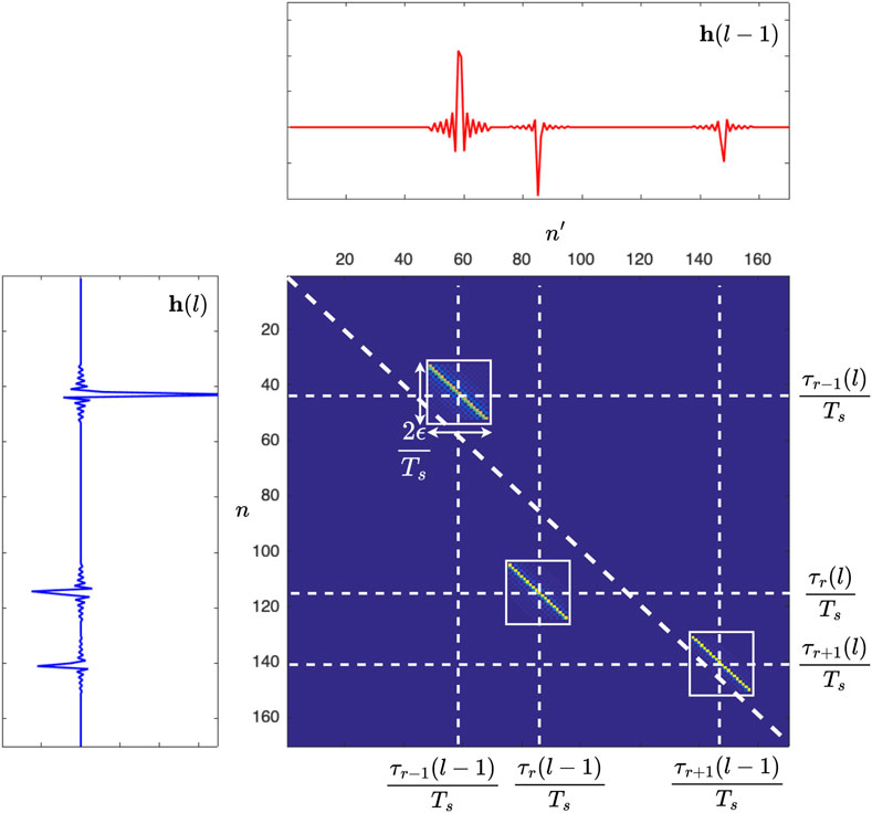
Figure 4. An example of an analytical location-variant transition matrix $\mathbf{A}(l)$ constructed from the early segments of two impulse responses, $\mathbf{h}(l)$ and $\mathbf{h}(l-1)$. The grid lines indicate the positions of the respective reflection TOAs.

4.2 Analytical location-invariant transition matrix model

For the application at hand, we anticipate employing a location-invariant transition matrix model as described in Equation 9 and illustrated in Figure 3B. We show that by using a location-invariant matrix, in which TOA intervals are defined to span the entire trajectory, we can reduce the necessity for accurate TOA estimates. This efficiency is achieved because these TOA intervals, along with TDOA estimates, can be obtained directly from $\mathbf{h}(0)$ to $\mathbf{h}(L-1)$ using the DTW-based method outlined in Section 4.3. In this section, we therefore derive a location-invariant transition matrix $\mathbf{A}$ from the definition of $\mathbf{A}(l)$ in Equation 29. As will be shown, location-invariance can be achieved within the limits of the trajectory under some assumptions.

In Equation 29, we observe two dependencies on $l$: in the TDOA ${\mathrm{\Delta }}_r(l)$ and in the set $\tilde{\mathcal{R}}(l,n)$. The dependency of ${\mathrm{\Delta }}_r(l)$ on $l$ disappears under the following conditions. As illustrated in Figure 5, under the assumptions of a far-field scenario where the (image) sources are far away in relation to the length of the trajectory, $a_r(l)/a_r(l-1)=1$ and ${\mathrm{\Delta }}_r(l)={\mathrm{\Delta }}_r$, meaning corresponding reflection TOAs are shifted by the same amount at each step along the trajectory. Consequently, the reflection TOA ${\tau }_r(l)$ can be approximated by the linear relation

${\tau }_r\left(l\right)={\tau }_r\left(0\right)+l{\mathrm{\Delta }}_r.(30)$

Figure 5

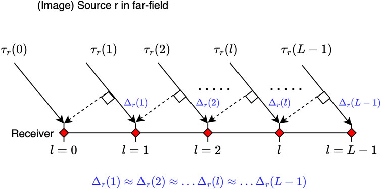
Figure 5. Illustration of the far-field assumption used to mitigate the dependence of ${\mathrm{\Delta }}_r(l)$ on $l$.

The dependence of $\tilde{\mathcal{R}}(l,n)$ on $l$ as defined in Equation 24 can be resolved as follows. The model in Equation 9 is required to hold for $l=1,\dots ,L-1$. Over this range of $l$, the components of reflection $r$ occupy the interval

${\mathcal{T}}_r=\left[{\tau }_{r|\mathrm{m}\mathrm{i}\mathrm{n}},{\tau }_{r|\mathrm{m}\mathrm{a}\mathrm{x}}\right](31)$

$\text{with}{\tau }_{r|\mathrm{m}\mathrm{i}\mathrm{n}}=\mathrm{m}\mathrm{i}\mathrm{n}\left({\tau }_r\left(1\right),{\tau }_r\left(L-1\right)\right)-ϵ,(32)$

${\tau }_{r|\mathrm{m}\mathrm{a}\mathrm{x}}=\mathrm{m}\mathrm{a}\mathrm{x}\left({\tau }_r\left(1\right),{\tau }_r\left(L-1\right)\right)+ϵ,(33)$

which can be understood as an extension of Equation 23.³

Based on Equation 31, we define the set similar to Equation 24 without the dependency on $l$:

$\tilde{\mathcal{R}}\left(n\right)=\left\{r\in \mathcal{R}\left|n\in \frac{{\mathcal{T}}_r}{T_s}\right.\right\}(34)$

The approximation in Equation 26 can then be replaced by

$h\left(l,n\right)\approx {\displaystyle \sum _{n^{\prime }}}{\displaystyle \sum _{r\in \tilde{\mathcal{R}}\left(n\right)}}\mathrm{s}\mathrm{i}\mathrm{n}\mathrm{c}\left(n-\frac{{\mathrm{\Delta }}_r}{T_s}-n^{\prime }\right)h\left(l-1,n^{\prime }\right)-e\left(l,n\right),(35)$

with the error term $e(l,n)$ redefined as

$e\left(l,n\right)={\displaystyle \sum _{n^{\prime }}}{\displaystyle \sum _{\begin{array}{c}r\in \tilde{\mathcal{R}}\left(n\right)\\ r^{\prime }\in \mathcal{R}\\ r^{\prime }\ne r\end{array}}}\mathrm{s}\mathrm{i}\mathrm{n}\mathrm{c}\left(n-\frac{{\mathrm{\Delta }}_r}{T_s}-n^{\prime }\right)\mathrm{s}\mathrm{i}\mathrm{n}\mathrm{c}\left(n^{\prime }-\frac{{\tau }_{r^{\prime }}\left(l-1\right)}{T_s}\right).(36)$

Again, the product $\mathrm{s}\mathrm{i}\mathrm{n}\mathrm{c}(n-{\mathrm{\Delta }}_r/T_s-n^{\prime })\mathrm{s}\mathrm{i}\mathrm{n}\mathrm{c}\left(n^{\prime }-({\tau }_{r^{\prime }}(l-1)/T_s)\right.$ in Equation 32 will be negligible if the two sinc-functions are misaligned, where $|n{T}_s-{\mathrm{\Delta }}_r-{\tau }_{r^{\prime }}(l-1)|>ϵ$. As shown in the Supplementary Appendix SB, this condition is equivalent to

${\mathcal{T}}_{r^{\prime }}^{-}\cap {\mathcal{T}}_r^{-}=\varnothing ,r^{\prime }\ne r(37)$

where

$\begin{array}{ll}\hfill {\mathcal{T}}_r^{-}& ={\mathcal{T}}_r-{\mathrm{\Delta }}_r\hfill \\ \hfill & =\left[{\tau }_{r|\mathrm{m}\mathrm{i}\mathrm{n}}^{-},{\tau }_{r|\mathrm{m}\mathrm{a}\mathrm{x}}^{-}\right],\hfill \end{array}(38)$

$\text{with}{\tau }_{r|\mathrm{m}\mathrm{i}\mathrm{n}}^{-}={\tau }_{r|\mathrm{m}\mathrm{i}\mathrm{n}}-{\mathrm{\Delta }}_r=\mathrm{m}\mathrm{i}\mathrm{n}\left({\tau }_r\left(0\right),{\tau }_r\left(L-2\right)\right)-ϵ-{\mathrm{\Delta }}_r,(39)$

${\tau }_{r|\mathrm{m}\mathrm{a}\mathrm{x}}^{-}={\tau }_{r|\mathrm{m}\mathrm{a}\mathrm{x}}-{\mathrm{\Delta }}_r=\mathrm{m}\mathrm{a}\mathrm{x}\left({\tau }_r\left(0\right),{\tau }_r\left(L-2\right)\right)+ϵ-{\mathrm{\Delta }}_r,(40)$

and the limits in Equations 39, 40 are obtained from Equations 32, 33, and ${\tau }_r(1)-{\mathrm{\Delta }}_r={\tau }_r(0)$ and ${\tau }_r(L-1)-{\mathrm{\Delta }}_r={\tau }_r(L-2)$ according to Equation 30. The condition in Equation 37 essentially states that the intervals that the individual reflections occupy over the range of the trajectory (with exclusion of the end point $l=L-1$) may not overlap. This can be understood as an extension of condition Equation 28 derived for the location-variant transition matrix. Neglecting $e(l,n)$ and referring back to the vector representation of RIRs in Equation 3, it can be seen that Equation 35 can be expressed in the form $\mathbf{h}(l)\approx \mathbf{A}\mathbf{h}(l-1)$ as anticipated in Equation 9, where the element of $\mathbf{A}$ at index $(n+1,n^{\prime }+1)$ is given by

$A_{n+1,n^{\prime }+1}={\displaystyle \sum _{r\in \tilde{\mathcal{R}}\left(n\right)}}\mathrm{s}\mathrm{i}\mathrm{n}\mathrm{c}\left(n-\frac{{\mathrm{\Delta }}_r}{T_s}-n^{\prime }\right).(41)$

if $\tilde{\mathcal{R}}(n)\ne \varnothing$ and otherwise $A_{n+1,n^{\prime }+1}(l)=0$.

Given the assumption of access to exact reflection TOAs ${\tau }_r(0)$ and ${\tau }_r(L-1)$, we estimate ${\mathrm{\Delta }}_r$ using Equation 30 as follows:

${\mathrm{\Delta }}_r=\frac{{\tau }_r\left(L-1\right)-{\tau }_r\left(0\right)}{L-1},(42)$

Note that from a conceptual point of view, the terms ${\tau }_r(l)$, ${\tau }_r(0)$, ${\tau }_r(L-1)-{\tau }_r(0)$, and $l/(L-1)$ in Equations 30 and 42 are comparable to ${\mathbf{n}}_r(l)$, ${\mathbf{n}}_r(0)$, ${\mathbf{n}}_r(L-1)-{\mathbf{n}}_r(0)$, and $\beta (l)$ in Equation 5, respectively. Note, however, that the latter are sample-based, while the former are defined in continuous time-shifts and can indeed be used to implement non-integer shifts by using the sinc-functions in Equation 29.

Keeping in mind Figures 3A and B, for an intuitive understanding of the relationship between $\mathbf{A}(l)$ and $\mathbf{A}$, we refer the reader to the toy example illustrated in Figure 6. Here, a trajectory with $L=3$ is considered, and matrices $\mathbf{A}(l)$ and $\mathbf{A}$ are, respectively, formed using Equations 29 or 41 with integer TOAs and $2ϵ/T_s=3$. It can be seen that the result of taking ${\mathbf{A}}^{L-1}$ yields an identical matrix to that of the multiplication of $\mathbf{A}(L-1)\cdots \mathbf{A}(2)\mathbf{A}(1)$ (Figures 6C, E). Furthermore, we note that the resulting matrix is equivalent to the matrix constructed using either Equations 29 or 41 for the case of $L=2$: a transition matrix between the start and end points of the trajectory as shown in Figure 3C.

Figure 6

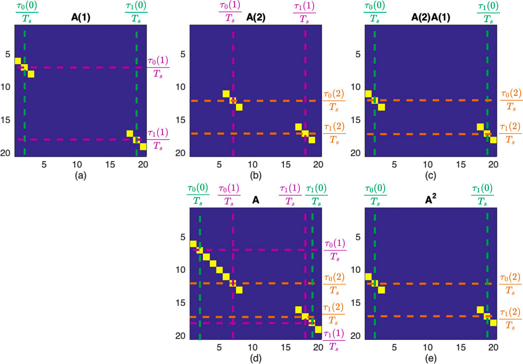
Figure 6. Illustration of the analytical transition matrices for a toy problem along a trajectory with $L=3$, with $\frac{2ϵ}{T_s}=3$ and integer reflection TOAs. Subfigures (a) and (b) show the location-variant matrices $\mathbf{A}(l)$ for $l=1$ and $l=2$, respectively. Subfigure (c) shows their product, A(2) A(1). Subfigure (d) shows the location-invariant matrix $\mathbf{A}$, while (e) depicts ${\mathbf{A}}^2$ (i.e., ${\mathbf{A}}^{L-1}$ for L = 3).

4.3 Dynamic Time Warping transition matrices

As it stands, the analytical solution proposed in Section 4.2 cannot be applied directly to RIRs and requires inherent knowledge of the TOAs in $\mathbf{h}(0)$ and $\mathbf{h}(L-1)$. Therefore, we propose an approach to estimate the matrix $\mathbf{A}$ using a DTW algorithm to temporally align elements in $\mathbf{h}(0)$ and $\mathbf{h}(L-1)$. DTW achieves temporal alignment by flexibly warping time, ensuring that similar patterns in the two sequences are matched, despite variations in timing. As discussed in Section 2.2, prior applications of DTW have involved linear interpolation between two impulse responses. However, the method proposed here builds upon the observation that the warp path derived from DTW can be linked to both the set $\tilde{\mathcal{R}}(n)$ and ${\tau }_r(L-1)-{\tau }_r(0)$, the latter of which is necessary for estimating ${\mathrm{\Delta }}_r$ via Equation 42. Leveraging these parameters enables the construction of an appropriate analytical location-invariant transition matrix $\mathbf{A}$, denoted as ${\widehat{\mathbf{A}}}_{\text{dtw}}$.

The DTW algorithm (Müller, 2007) involves computing an accumulated cost matrix $\mathbf{D}\in {\mathbb{R}}^{(N+1)\times (N+1)}$, representing the cumulative costs of aligning each element in $\mathbf{h}(L-1)$ with each element in $\mathbf{h}(0)$, respectively, indexed by $n$ and $n^{\prime }$. Here, the cost is defined as the Euclidean distance $\Vert h(L-1,n)-h(0,n^{\prime }){\Vert }_2$, and $\mathbf{D}$ is constructed using the recurrence relation

$D_{n+2,n^{\prime }+2}=\Vert h\left(L-1,n\right)-h\left(0,n^{\prime }\right){\Vert }_2+\min \left\{D_{n+1,n^{\prime }+2},D_{n+2,n^{\prime }+1},D_{n+1,n^{\prime }+1}\right\},(43)$

which is initialized such that $D_{\mathrm{1,1}}=0$, while $D_{n+\mathrm{2,1}}$ and $D_{1,n^{\prime }+2}$ are set to $\infty$ for all $n$ and $n^{\prime }$, respectively⁴. Owing to the prominent reflection peaks in the structure of early RIRs, the matrix $\mathbf{D}$ will be formed with grid-like entries (Figure 7B)

Figure 7

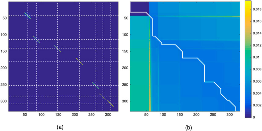
Figure 7. (A) Location-invariant matrix $\mathbf{A}$ for the special case of $L=2$ and (B) accumulated distance matrix $\mathbf{D}$ constructed from $\mathbf{h}(0)$ and $\mathbf{h}(L-1)$ overlaid with DTW warp path (white line).

A warp path, denoted by pairs of indices $(n+2,n^{\prime }+2)$ representing optimal alignment in the sense of smallest accumulated cost, is established by backtracking from $D_{N+2,N+2}$ to $D_{\mathrm{2,2}}$. The recurrence relation in Equation 43 guarantees a monotonically increasing order, thus ensuring that peaks in sequences are mapped in the same order they appear, preserving temporal correspondence during alignment. Note that a single point in one sequence can correspond to multiple points in the other, and vice versa. An illustration of the warp path through $\mathbf{D}$ can be seen in Figure 7B.

The elements along the horizontal and vertical “gridlines” in $\mathbf{D}$ contain local maxima values, whose row and column indices should respectively correspond to integer estimates of reflection TOA time-shift indices $\frac{{\tau }_r(L-1)}{T_s}$ and $\frac{{\tau }_r(0)}{T_s}$. The elements at the intersections of these “gridlines” represent local minima in $\mathbf{D}$, signifying potential alignment points between reflection peaks in $\mathbf{h}(L-1)$ and $\mathbf{h}(0)$. Consequently, the warp path tends to traverse these intersections in a diagonal manner, guided by the minimization of alignment costs. Here, a clear link between the shape of the warp path through $\mathbf{D}$ (Figure 7B) and the analytical matrix $\mathbf{A}$ constructed using Equation 41 for $L=2$ (Figure 7A) becomes apparent. Recall that the case of $L=2$ results in a matrix $\mathbf{A}$ that maps the RIR at the start of the trajectory to the RIR at its end (Figure 3C).

In order to use the shape of the warp path through $\mathbf{D}$, we need to construct a matrix $\mathbf{W}\in {\mathbb{R}}^{N\times N}$, with ones placed at the indices corresponding to the pairs in the warp path and zeros elsewhere:

$W_{n+1,n^{\prime }+1}=\left\{\begin{array}{cc}1\hfill & \text{if\hspace{0.17em}}\left(n+2,n^{\prime }+2\right)\text{\hspace{0.17em}is\hspace{0.17em}in\hspace{0.17em}the\hspace{0.17em}warp\hspace{0.17em}path}\hfill \\ 0\hfill & \text{otherwise}\hfill \end{array}\right.$

Such a matrix $\mathbf{W}$ is shown in Figure 8D for the previous toy problem with integer TOAs and $\frac{2ϵ}{T_s}=3$. It can be seen that the diagonal segments of $\mathbf{W}$ are consistent with the toy problem matrix ${\mathbf{A}}^{L-1}$, which is again displayed in Figure 8B. We therefore propose to leverage the positions of the diagonal segments in $\mathbf{W}$ to obtain the estimates of ${\mathrm{\Delta }}_r$ and $\tilde{\mathcal{R}}(n)$ needed to construct $\mathbf{A}$ as follows.

Figure 8

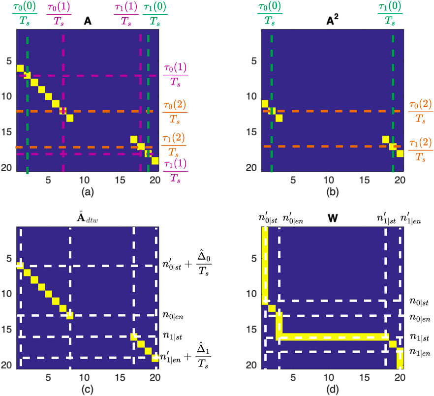
Figure 8. Illustration of the analytical transition matrices for a toy problem along a trajectory with $L=3$, with $\frac{2ϵ}{T_s}=3$ and integer reflection TOAs. Subfigure (a) shows the location-invariant matrix A, while (b) depicts ${\mathbf{A}}^2$ (i.e., ${\mathbf{A}}^{L-1}$ for $L=3$). Subfigures (c) and (d) respectively present the matrix $\mathbf{W}$, derived from the DTW warp path, and the estimated location-invariant matrix ${\widehat{\mathbf{A}}}_{\text{dtw}}$.

Firstly, integer estimates of $({\tau }_r(L-1)-{\tau }_r(0))/T_s$ are obtained by measuring the “distances” (number of elements) from the diagonal segments in $\mathbf{W}$ to the main diagonal. These estimates can in turn be used to find estimates of ${\mathrm{\Delta }}_r$ using the relation in Equation 42 and the known sampling period $T_s$. We employ ${\widehat{\mathrm{\Delta }}}_r$ and ${\widehat{\tau }}_r$ to distinguish the estimates found in this manner:

${\widehat{\mathrm{\Delta }}}_r=\frac{{\widehat{\tau }}_r\left(L-1\right)-{\widehat{\tau }}_r\left(0\right)}{L-1},(44)$

Secondly the start and end indices of the diagonal segments, denoted, respectively, as $(n_{r|\text{st}},n_{r|\text{st}}^{\prime })$ and $(n_{r|\text{en}},n_{r|\text{en}}^{\prime })$, are retrieved. These indices are then used to find a suitable estimate of the range ${\mathcal{T}}_r$ for the set $\tilde{\mathcal{R}}(n)$ in Equation 34 as

${\widehat{\mathcal{T}}}_r=\left[{\widehat{\tau }}_{r|\mathrm{m}\mathrm{i}\mathrm{n}},{\widehat{\tau }}_{r|\mathrm{m}\mathrm{a}\mathrm{x}}\right](45)$

${\widehat{\tau }}_{r|\mathrm{m}\mathrm{i}\mathrm{n}}=T_s\cdot \mathrm{m}\mathrm{i}\mathrm{n}\left(n_{r|\text{st}}^{\prime }+\frac{{\widehat{\mathrm{\Delta }}}_r}{T_s\left(L-1\right)},n_{r|\text{st}}\right),(46)$

${\widehat{\tau }}_{r|\mathrm{m}\mathrm{a}\mathrm{x}}=T_s\cdot \mathrm{m}\mathrm{a}\mathrm{x}\left(n_{r|\text{en}},n_{r|\text{en}}^{\prime }+\frac{{\widehat{\mathrm{\Delta }}}_r}{T_s\left(L-1\right)}\right),(47)$

It should be ensured that the estimated ranges still result in the condition in Equation 37 being met—that is, that corresponding column ranges do not overlap. Finally, we construct the matrix ${\widehat{\mathbf{A}}}_{\text{dtw}}$ using Equations 41 and 34 with ${\mathrm{\Delta }}_r={\widehat{\mathrm{\Delta }}}_r$ and ${\mathcal{T}}_r={\widehat{\mathcal{T}}}_r$ where ${\widehat{\mathrm{\Delta }}}_r\text{and}{\widehat{\mathcal{T}}}_r$ are obtained using Equations 44 to 47. Figure 8C illustrates an example of a matrix obtained using this method for the previous toy problem. It is apparent that ${\widehat{\mathbf{A}}}_{\text{dtw}}$ closely aligns with the desired $\mathbf{A}$ matrix shown in Figure 8A. Importantly, the described method allows us to derive $\mathbf{A}$ without needing to explicitly estimate individual TOAs.

5 Simulations

In this section, we systematically evaluate the performance of transition matrices $\mathbf{A}$ and ${\widehat{\mathbf{A}}}_{\text{dtw}}$ in state-space RIR estimation. The algorithms considered are summarized in Table 1, with $\mathbf{\text{LI}}-\mathbf{A}$ and $\mathbf{\text{KF}}-\alpha$ serving as reference methods, and $\mathbf{\text{KF}}-\mathbf{A}$ and $\mathbf{\text{KF}}-{\widehat{\mathbf{A}}}_{\text{dtw}}$ representing our primary contributions from the proposed methods outlined in Section 3. In Section 5.1, we provide details on the experimental setup, including the simulated acoustic environment, Kalman filter parameters, and the performance measure used. The results of the experiments are presented in Section 6.

Table 1

Table 1. Description of the algorithms compared in the experimental results.

5.1 Acoustic environment

For simplicity, we consider a box-shaped room with dimensions bounded by $[\mathrm{0,4.50}]\times [\mathrm{0,5.80}]\times [\mathrm{0,2.90}]$ m. We place a fixed-position sound source at $[1.05,2.98,1.17]$ m, and define a linear trajectory for the microphone spanning approximately 0.7 m, starting at $[1.94,3.10,1.09]$ m and ending at $[1.99,2.95,0.37]$ m. Along this trajectory, we have established that all first-order reflections arrive in the same order. The set-up is shown in Figure 9.

Figure 9

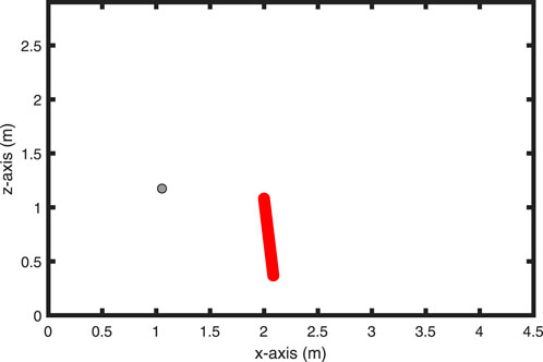
Figure 9. 2-D illustration depicting the source position and trajectory of the microphone within a box-shaped room, as utilized for simulations.

At a standard speech sampling rate of 16 kHz (Nophut et al., 2024) and with a microphone velocity of 0.25 m/s, the ISM (Allen and Berkley, 1979) is used to simulate the ground-truth early RIRs $\mathbf{h}(l)$, including reflections up to the second order, at various points along the trajectory. Subsequently, the observed output signal $y_{\mathrm{\Omega }}(l)$ is obtained using Equation 11 for a given input $x_{\mathrm{\Omega }}(l)$ and measurement noise $v_{\mathrm{\Omega }}(l)\sim \mathcal{N}(0,{\sigma }_y^2)$, where the variance ${\sigma }_v^2$ is adjusted based on the experimental conditions. White Gaussian noise is chosen as the input signal, denoted as $x(l)\sim \mathcal{N}(0,{\sigma }_x^2)$, with the variance ${\sigma }_x^2$ set as $10{\log }_{10}({\sigma }_x^2)=-20$ dB.

5.2 Kalman filter parameters

As outlined in Section 3.1, the Kalman filter relies on specific input parameters for its operation. These parameters include the process noise covariance matrix $\mathbf{Q}$ and the variance of the measurement noise $R$. Additionally, the filter requires initialization with a state estimate ${\widehat{\mathbf{h}}}^{+}(0)$ and an initial guess for the state estimation error covariance matrix ${\mathbf{P}}^{+}(0)$.

Given the assumption of knowledge of the RIR at the start of the trajectory $\mathbf{h}(0)$, the filter is initialized with ${\widehat{\mathbf{h}}}^{+}(0)=\mathbf{h}(0)$. Since we are simulating measurement noise with variance ${\sigma }_v^2$, we set $R={\sigma }_v^2$. As previously mentioned, $R$ can in practice potentially be estimated using background noise recordings. The appropriate $\mathbf{A}$ matrix is selected for each algorithm, as outlined in Table 1, with the considered width $2ϵ$ of the $\mathrm{s}\mathrm{i}\mathrm{n}\mathrm{c}$ functions in the proposed analytical transition matrices set to $\frac{2ϵ}{T_s}=20$. It was found that for the reference Kalman filter, a transition factor of $\alpha =1$ was suitable, and varying this did not change the results in a significant manner. After some initial testing of the Kalman filter, the tuning parameter $\mathbf{Q}$ was chosen as $\mathbf{Q}={\sigma }_w^2\mathbf{I}$, where $\mathbf{I}$ is an identity matrix and $10\log ({\sigma }_w^2)=-30$ dB.

5.3 Performance measure

In assessing the accuracy of our estimated RIRs ${\widehat{\mathbf{h}}}^{+}(l)$, we employ the normalized misalignment ${\mathcal{M}}_{\text{dB}}(l)$. This metric is defined thus:

${\mathcal{M}}_{\text{dB}}\left(l\right)=20{\log }_{10}\left(\frac{\Vert {\widehat{\mathbf{h}}}^{+}\left(l\right)-\mathbf{h}\left(l\right){\Vert }_2}{\Vert \mathbf{h}\left(l\right){\Vert }_2}\right).$

Here, $\mathbf{h}(l)$ represents the ground truth early RIRs.

5.4 Experiments

We categorize experiments into the following four sets to evaluate algorithm performance.

$•$ Experiment 1: Ideal case. In the first set of experiments, we examine the “ideal” scenario where no noise is present on the observed output signal $y_{\mathrm{\Omega }}(l)$ $({\sigma }_v^2=0)$ and every sample along the trajectory is considered $(\mathrm{\Omega }=1)$. Simulated RIRs exclusively include first-order reflections.

$•$ Experiment 2: Noise sensitivity. Building upon the setup in Experiment 1 with $\mathrm{\Omega }=1$ and only first-order reflections included, the second set of experiments evaluates algorithm robustness when different noise levels are added to the observed output signal—that is, varying $\text{SNR}=\{\mathrm{6,0},-6\}$ dB.

$•$ Experiment 3: Spatial sampling effects. The third set of experiments employs different spatial downsampling factors $\mathrm{\Omega }$ to assess the impact of using fewer data points along the trajectory. In this case, we once again consider ${\sigma }_v^2=0$ and only first-order reflections, while varying $\mathrm{\Omega }=\{\mathrm{2,8,32}\}$. Note that $\mathrm{\Omega }=2$ corresponds to $50\%$ of the samples along the trajectory being used.

$•$ Experiment 4: Second-order reflections included. The final set of experiments investigates the inclusion of second-order reflections in the RIRs and the corresponding simulated observed signal. We once again examine the “ideal” scenario where no noise is present on the observed output signal $y_{\mathrm{\Omega }}(l)$ $({\sigma }_v^2=0)$ and every sample along the trajectory is considered $(\mathrm{\Omega }=1)$. Please note that the analytical transition matrix $\mathbf{A}$ is still constructed solely using first-order TOAs, as not all second-order reflections meet the necessary assumptions along the given trajectory. As a robustness measure, after constructing $\mathbf{A}$, ones are added along the main diagonal in any part of the matrix with empty rows. This step ensures that second-order reflections are not entirely discarded. On the other hand, the DTW algorithm operates directly on the RIRs, and thus, when constructing ${\widehat{\mathbf{A}}}_{\text{dtw}}$, it inherently assumes that all reflections arrive in the same order in $\mathbf{h}(0)$ and $\mathbf{h}(L-1)$. In other words, it may incorrectly associate some reflections in $\mathbf{h}(0)$ and $\mathbf{h}(L-1)$ as belonging to the same image source.

6 Results

We present the results corresponding to the experiments outlined above. The reader is urged to take careful note of the different $y$-axis scaling in the presented results.

6.1 Result 1: ideal case

The results of Experiment 1 are presented at the top of Figure 10, where the normalized misalignment ${\mathcal{M}}_{\text{dB}}(l)$ between the ground-truth RIR $\mathbf{h}(l)$ and the estimated RIR $\widehat{\mathbf{h}}(l)$ is displayed for the various algorithms at different positions along the trajectory. The bottom of Figure 10 shows the start and end point RIRs used to obtain our transition matrices. This is provided to give the reader an idea of how the source and reflection TOAs change over the trajectory. Furthermore, it can be seen from the labeled TOAs that there are no overlapping intervals, which aligns with our assumptions.

Figure 10

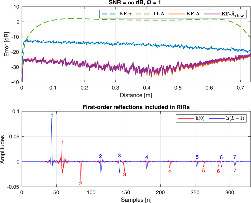
Figure 10. (Top) Result 1: Normalized misalignment along the trajectory between the “ground-truth” RIR $\mathbf{h}(l)$ and the estimated RIR $\widehat{\mathbf{h}}(l)$ using algorithms detailed in Table 1. This is for the case of a noiseless observed output signal $y_{\mathrm{\Omega }}(l)$. (Bottom) Simulated RIRs corresponding to the start and end of the trajectory, denoted as $\mathbf{h}(0)$ and $\mathbf{h}(L-1)$, respectively. Peaks corresponding to the same source or reflection are labeled by the same number in each RIR.

At the beginning of the trajectory, all algorithms exhibit zero error owing to their initialization with a known RIR $\mathbf{h}(0)$. Following a subsequent steep increase in error, distinctive properties of the curves resulting from the different algorithms become evident. The reference Kalman filter algorithm $(\mathbf{\text{KF}}-\alpha )$, which utilizes a transition factor of $\alpha =1$ and relies solely on microphone observations, demonstrates a gradual decrease in error throughout the remainder of the trajectory. Excluding the start and end segments, it can be observed that Algorithm $\mathbf{\text{LI}}-\mathbf{A}$, whose performance solely relies on the model of $\mathbf{A}$, results in an error curve with a subtle dip in it. This non-monotonic behavior can be attributed to the position of the direct source relative to the linear microphone trajectory (Figure 9) and the fact that the source is not sufficiently in the far-field for our assumption that TDOAs remain approximately constant to hold. Toward the end of the trajectory, Algorithm $\mathbf{\text{LI}}-\mathbf{A}$ exhibits a rapid decrease in error. This is because the matrix $\mathbf{A}$ is derived from accurate TOAs at the start and end of the trajectory, and therefore estimates should most closely align with the ground-truth RIRs around these positions.

In general, changes in the error curve of the Kalman filter algorithms using a transition matrix ($\mathbf{\text{KF}}-\mathbf{A}$ and $\mathbf{\text{KF}}-{\widehat{\mathbf{A}}}_{\text{dtw}}$) correlate with changes in the error curve of Algorithm $\mathbf{\text{LI}}-\mathbf{A}$. However, a more significant dip in error is observed, and the curves nearly converge with those of Algorithm $\mathbf{\text{KF}}-\alpha$ at the end of the trajectory. This behavior may be a result of the rapid convergence of $\mathbf{\text{KF}}-\mathbf{A}$ and $\mathbf{\text{KF}}-{\widehat{\mathbf{A}}}_{\text{dtw}}$ under ideal conditions (i.e., no noise), making the Kalman filter more sensitive to the degradation of the transition matrix model accuracy.

If we now consider the relative performance of the algorithms, we note that the Kalman filter employing “ideal” analytical transition matrix Algorithm $\mathbf{\text{KF}}-\mathbf{A}$ showcases a substantial improvement which is, on average, approximately $-15$ dB compared to the reference Kalman filter, Algorithm $\mathbf{\text{KF}}-\alpha$. Importantly, similar improvement extends to the case where the analytical transition matrix approximated using DTW is used—Algorithm $\mathbf{\text{KF}}-{\widehat{\mathbf{A}}}_{\text{dtw}}$. Moreover, the advantage of employing a state-space model over a linear interpolation method becomes evident from the comparatively poor overall results of Algorithm $\mathbf{\text{LI}}-\mathbf{A}$. The observed enhancements in accuracy support our preliminary hypothesis: the combination of room acoustic model-based interpolation and a data-driven state-space model provides a more accurate approach to early RIR estimation.

6.2 Result 2: noise sensitivity

The results of Experiment 2 are presented in Figure 11 and once again exhibit error curve shapes consistent with those observed in Experiment 1. However, as anticipated, overall performance is worse, except for Algorithm $\mathbf{\text{LI}}-\mathbf{A}$, which remains unaffected since it does not rely on the noisy microphone measurements. Additionally, we observe slower convergence and less pronounced dips in the error curves of the algorithms $\mathbf{\text{KF}}-\mathbf{A}$ and $\mathbf{\text{KF}}-{\widehat{\mathbf{A}}}_{\text{dtw}}$ compared to the noiseless case. This is likely because the less reliable observations prevent convergence to such low error levels in the first place, making the dips less noticeable.

Figure 11

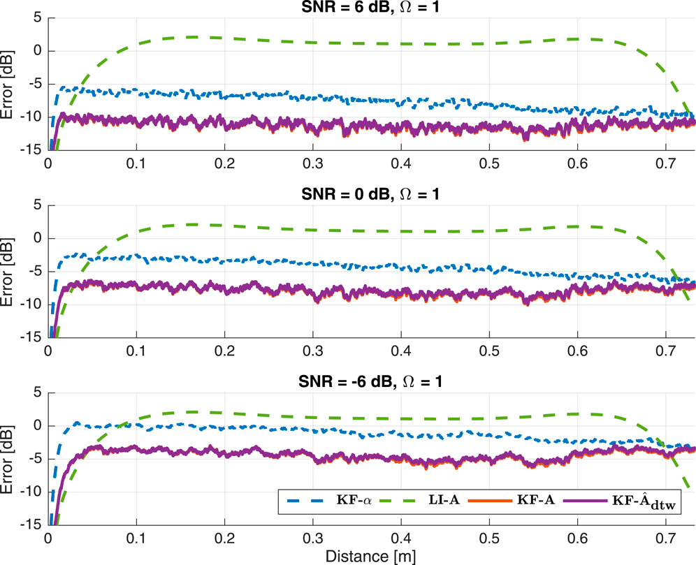
Figure 11. Result 2: Normalized misalignment along the trajectory between the “ground-truth” RIR $\mathbf{h}(l)$ and the estimated RIR $\widehat{\mathbf{h}}(l)$ using algorithms detailed in Table 1. This assessment is conducted for different levels of noise added to the observed output signal $y_{\mathrm{\Omega }}(l)$.

It is evident that even under poor SNR conditions, our methods consistently outperform both reference algorithms. Notably, at an SNR of $-6$ dB, an average of approximately $-5$ dB difference persists, further underscoring the advantages of the proposed approach, even when measurements contain high levels of noise.

6.3 Result 3: spatial sampling effects

The results of Experiment 3 are presented in Figure 12. As fewer measurements are used, the disparity between the results obtained using the linear interpolation method and those obtained using a Kalman filter naturally diminishes. Additionally, the performance of the reference Kalman filter $(\mathbf{\text{KF}}-\alpha )$ deteriorates more rapidly than that of our proposed methods ($\mathbf{\text{KF}}-\mathbf{A}$ and $\mathbf{\text{KF}}-{\widehat{\mathbf{A}}}_{\text{dtw}}$). We further note an apparent shift in the position of the dip in the error curve of Algorithms $\mathbf{\text{KF}}-\mathbf{A}$ and $\mathbf{\text{KF}}-{\widehat{\mathbf{A}}}_{\text{dtw}}$ as fewer samples are used. This is likely a consequence of the change in how often the state equation is propagated.

Figure 12

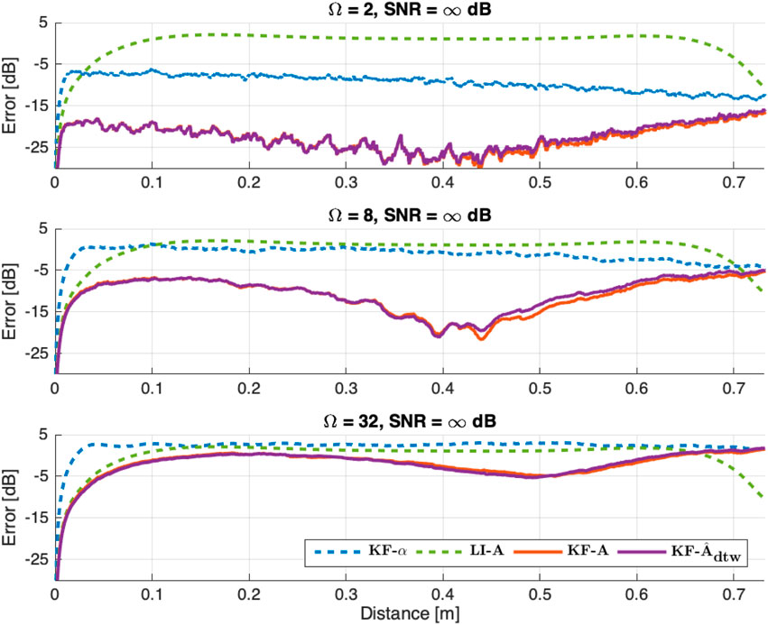
Figure 12. Result 3: Normalized misalignment along the trajectory between the “ground-truth” RIR $\mathbf{h}(l)$ and the estimated RIR $\widehat{\mathbf{h}}(l)$ using algorithms detailed in Table 1. This is for the case of a noiseless observed output signal $y_{\mathrm{\Omega }}(l)$ with different spatial sampling along the trajectory as a function of $\mathrm{\Omega }$.

For $\mathrm{\Omega }=8$, equivalent to approximately $12.5\%$ of the available sampling points, Algorithms $\mathbf{\text{KF}}-\alpha$ and $\mathbf{\text{LI}}-\mathbf{A}$ exhibit similar performance, while our proposed algorithms consistently outperform both by an average of approximately $-12$ dB. Despite the trivial choice between the two reference methods when only a small number of measurements are available, as demonstrated by the case of $\mathrm{\Omega }=32$ (equivalent to $3.13\%$ of sampling points), our proposed method still demonstrates an overall improvement in performance.

6.4 Result 4: second-order reflections included

The results of Experiment 4 are shown at the top of Figure 13. It is important to recall that in Experiment 4, the analytical transition matrix $\mathbf{A}$ used in Algorithm $\mathbf{\text{KF}}-\mathbf{A}$ is still constructed using only first-order TOAs. This is because not all second-order reflections meet the necessary assumptions along the given trajectory, as indicated by the reflection TOA labels toward the end of the RIR at the bottom of Figure 13—for example, the interval over which reflection 6 moves overlaps with reflections 7, 8, and 9. However, by adding ones along the diagonal of $\mathbf{A}$ in any empty rows, we ensure that second-order reflections are not entirely discarded. This allows us to leverage prior knowledge, even if incomplete, and explains the strong convergence with Algorithm $\mathbf{\text{KF}}-\alpha$ toward the end of the trajectory. That being said, Algorithm $\mathbf{\text{KF}}-\mathbf{A}$ still demonstrates an average improvement of approximately $-7$ dB over Algorithm $\mathbf{\text{KF}}-\alpha$.

Figure 13

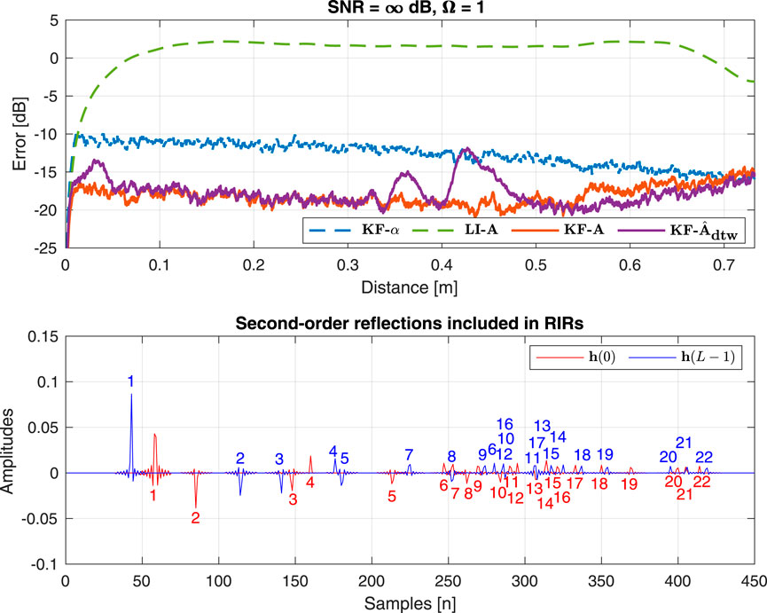
Figure 13. (Top) Result 4: Normalized misalignment along the trajectory between the “ground-truth” RIR $\mathbf{h}(l)$ and the estimated RIR $\widehat{\mathbf{h}}(l)$ using algorithms detailed in Table 1. This is for the case of a noiseless observed output signal $y_{\mathrm{\Omega }}(l)$ with simulated RIRs inclusive of second-order reflections. (Bottom) Simulated RIRs corresponding to the start and end of the trajectory, denoted as $\mathbf{h}(0)$ and $\mathbf{h}(L-1)$, respectively. Peaks corresponding to the same source or reflection are labeled by the same number in each RIR.

It is important to reiterate that in estimating the matrix ${\widehat{\mathbf{A}}}_{\text{dtw}}$, we directly utilize the RIRs $\mathbf{h}(0)$ and $\mathbf{h}(L-1)$, thus implicitly incorporating second-order reflection information. However, in this case, not all second-order reflections adhere to the assumption that the time intervals’ individual reflections occupy over the trajectory do not overlap. Given that DTW inherently maps sequences in a monotonic manner, assuming consistent order among significant points like peaks, certain reflection peaks might be incorrectly mapped between RIRs. Consequently, the points along the trajectory where second-order reflections in the ground-truth RIRs begin to overlap likely correspond to the jumps observed in the error curve of Algorithm $\mathbf{\text{KF}}-{\widehat{\mathbf{A}}}_{\text{dtw}}$. Nonetheless, this serves as a robust test demonstrating that despite deviations from certain assumptions regarding all reflections, the proposed estimated matrix still yields an overall enhancement over Algorithm $\mathbf{\text{KF}}-\alpha$.

7 Conclusion

This paper investigates the estimation of early segments of time-varying RIRs through a state-space model incorporating the ISM within the state transition matrix. Simulation results indicate that this approach outperforms both RIR interpolation and a purely data-driven state-space model using a transition factor. Moreover, a practical method for estimating such a matrix has been proposed and has a similar performance to the “ideal” analytical transition matrix derived. It is important to acknowledge that certain assumptions inherent to our method limit its application within specific areas of a room. This necessitates further research in order to improve the robustness of the approach, potentially through adaptive estimation of the transition matrix. Furthermore, experimental validation using real measurement data is required to assess the effectiveness of the proposed approach in real-world scenarios.

Data availability statement

The raw data supporting the conclusions of this article will be made available by the authors, without undue reservation.

Author contributions

KM: conceptualization, formal analysis, investigation, methodology, validation, writing–original draft, and writing–review and editing. TD: conceptualization, methodology, supervision, writing–original draft, and writing–review and editing. RA: conceptualization, supervision, writing–original draft, and writing–review and editing. TV: conceptualization, funding acquisition, supervision, and writing–review and editing.

Funding

The authors declare that financial support was received for the research, authorship, and/or publication of this article. This work was supported by

$•$ The European Research Council under the European Union’s Horizon 2020 research and innovation program/ERC Consolidator Grant: SONORA (no. 773268). This paper reflects only the authors’ views, and the EU is not liable for any use that may be made of the contained information.

$•$ KU Leuven Internal Funds C14/21/075 “A holistic approach to the design of integrated and distributed digital signal processing algorithms for audio and speech communication devices”

$•$ FWO Research Project: “The Boundary Element Method as a State-Space Realization Problem” (G0A0424N)

Conflict of interest

The authors declare that the research was conducted in the absence of any commercial or financial relationships that could be construed as a potential conflict of interest.

Publisher’s note

All claims expressed in this article are solely those of the authors and do not necessarily represent those of their affiliated organizations, or those of the publisher, the editors, and the reviewers. Any product that may be evaluated in this article, or claim that may be made by its manufacturer, is not guaranteed or endorsed by the publisher.

Supplementary material

The Supplementary Material for this article can be found online at: https://www.frontiersin.org/articles/10.3389/frsip.2024.1426082/full#supplementary-material

Footnotes

¹For notational convenience when working with an interval $[a,b]$, we introduce $\frac{[a,b]}{c}$ to represent $[\frac{a}{c},\frac{b}{c}]$ (see Equations 24 and 34), and $[a,b]-c$ to represent $[a-c,b-c]$ (Equation 38).

²In the special case that ${\tau }_r(l)/T_s$ and ${\tau }_r(l-1)/T_s$ are integers, the sinc-functions are sampled symmetrically around their peak, which implies that all but the peak sample lie at the zero crossings of the sinc-functions, resulting in diagonal submatrices.

³Note that if ${\mathrm{\Delta }}_r<2ϵ$, we find that ${\mathcal{T}}_r={\bigcup }_{l=1}^{L-1}{\mathcal{T}}_r(l)$.

⁴In this paper, matrices are indexed from (1,1), following the convention of many programming languages. However, our RIR sequences are indexed from 0. To align with the zero-based indexing of our RIRs and accommodate the additional row and column used solely for initialization, we index the entries of the accumulated cost matrix as $D_{n+2,n^{\prime }+2}$

References

Ajdler, T., Sbaiz, L., and Vetterli, M. (2007). Dynamic measurement of room impulse responses using a moving microphone. J. Acoust. Soc. Amer. 122, 1636–1645. doi:10.1121/1.2766776

PubMed Abstract | CrossRef Full Text | Google Scholar

Allen, J. B., and Berkley, D. A. (1979). Image method for efficiently simulating small-room acoustics. J. Acoust. Soc. Amer. 65, 943–950. doi:10.1121/1.382599

CrossRef Full Text | Google Scholar

Antonello, N., De Sena, E., Moonen, M., Naylor, P. A., and Van Waterschoot, T. (2017). Room impulse response interpolation using a sparse spatio-temporal representation of the sound field. IEEE/ACM Trans. Audio Speech Lang. Process. 25, 1929–1941. doi:10.1109/taslp.2017.2730284

CrossRef Full Text | Google Scholar

Antweiler, C., and Symanzik, H. G. (1995). Simulation of time variant room impulse responses. Proc. 1995 IEEE Int. Conf. Acoust. Speech, Signal Process. (ICASSP ’95) 5, 3031–3034. doi:10.1109/icassp.1995.479484

CrossRef Full Text | Google Scholar

Antweiler, C., Telle, A., Vary, P., and Enzner, G. (2012). “Perfect-sweep NLMS for time-variant acoustic system identification,” in Proc. 2012 IEEE int. Conf. Acoust., speech, signal process. (ICASSP ’12), 517–520. doi:10.1109/ICASSP.2012.6287930

CrossRef Full Text | Google Scholar

Borra, F., Gebru, I. D., and Markovic, D. (2019). “Soundfield reconstruction in reverberant environments using higher-order microphones and impulse response measurements,” in Proc. 2021 IEEE int. Conf. Acoust., speech, signal process. (ICASSP ’19), 281–285. doi:10.1109/ICASSP.2019.8682961

CrossRef Full Text | Google Scholar

Bruschi, V., Nobili, S., Cecchi, S., and Piazza, F. (2020). An innovative method for binaural room impulse responses interpolation. Audio Eng. Soc. Conv. 148.

Google Scholar

Carty, B. (2010). Movements in binaural space: issues in HRTF interpolation and reverberation, with applications to computer music. National University of Ireland Maynooth. Ph.D. thesis.

Google Scholar

Cherniakov, M. (2003). An introduction to parametric digital filters and oscillators. New York: John Wiley and Sons.

Google Scholar

Crocco, M., and Bue, A. D. (2015). Room impulse response estimation by iterative weighted l1-norm. Proc. 23rd Eur. Signal Process. Conf. (EUSIPCO ’15), 1895–1899. doi:10.1109/EUSIPCO.2015.7362713

CrossRef Full Text | Google Scholar

Das, O., Calamia, P., and Gari, S. V. A. (2021). “Room impulse response interpolation from a sparse set of measurements using a modal architecture,” in Proc. 2021 IEEE int. Conf. Acoust., speech, signal process. (ICASSP ’21), 960–964. doi:10.1109/ICASSP39728.2021.9414399

CrossRef Full Text | Google Scholar

Elko, G. W., Diethorn, E., and Gänsler, T. (2003). “Room impulse response variation due to temperature fluctuations and its impact on acoustic echo cancellation,” in Proc. 2003 int. Workshop acoustic echo noise control (IWAENC ’03), 67–70.

Google Scholar

Enzner, G. (2008). Analysis and optimal control of lms-type adaptive filtering for continuous-azimuth acquisition of head related impulse responses, 393–396. doi:10.1109/ICASSP.2008.4517629

CrossRef Full Text | Google Scholar

Enzner, G. (2010). “Bayesian inference model for applications of time-varying acoustic system identification,” in Proc. 18th European signal process. Conf. (EUSIPCO ’10), 2126–2130.

Google Scholar

Evers, C., Löllmann, H. W., Mellmann, H., Schmidt, A., Barfuss, H., Naylor, P. A., et al. (2020). The locata challenge: acoustic source localization and tracking. IEEE/ACM Trans. Audio Speech Lang. Process. 28, 1620–1643. doi:10.1109/taslp.2020.2990485

CrossRef Full Text | Google Scholar

Garcia-Gomez, V., and Lopez, J. J. (2018). “Binaural room impulse responses interpolation for multimedia real-time applications,” in AES 144th convention.

Google Scholar

Geldert, A., Meyer-Kahlen, N., and Schlecht, S. J. (2023). “Interpolation of spatial room impulse responses using partial optimal transport,” in Proc. 2023 IEEE int. Conf. Acoust., speech, signal process. (ICASSP ’23), 1–5.

CrossRef Full Text | Google Scholar

Hahmann, M., and Fernandez-Grande, E. (2022). A convolutional plane wave model for sound field reconstruction. J. Acoust. Soc. Amer. 152 (5), 3059–3068. doi:10.1121/10.0015227

CrossRef Full Text | Google Scholar

Hahn, N., and Spors, S. (2015). Continuous measurement of impulse responses on a circle using a uniformly moving microphone, 2536–2540. doi:10.1109/EUSIPCO.2015.7362842

CrossRef Full Text | Google Scholar

Haneda, Y., Kaneda, Y., and Kitawaki, N. (1999). Common-acoustical-pole and residue model and its application to spatial interpolation and extrapolation of a room transfer function. IEEE Trans. Speech, Audio Process 7, 709–717. doi:10.1109/89.799696

CrossRef Full Text | Google Scholar

Hoskins, R. F. (2009). Delta functions: introduction to generalised functions. Woodhead Publishing.

Google Scholar

Karakonstantis, X., Caviedes-Nozal, D., Richard, A., and Fernandez-Grande, E. (2024). Room impulse response reconstruction with physics-informed deep learning. J. Acoust. Soc. Amer. 155 (2), 1048–1059. doi:10.1121/10.0024750

CrossRef Full Text | Google Scholar

Katzberg, F., Mazur, R., Maass, M., Böhme, M., and Mertins, A. (2018). “Spatial interpolation of room impulse responses using compressed sensing,” in Proc. 2018 int. Workshop acoustic signal enhancement (IWAENC ’18), 426–430. doi:10.1109/IWAENC.2018.8521390

CrossRef Full Text | Google Scholar

Kearney, G., Masterson, C., Adams, S., and Boland, F. (2009). “Dynamic time warping for acoustic response interpolation: possibilities and limitations,” in Proc. 17th European signal process. Conf. (EUSIPCO ’09), 705–709.

Google Scholar

Kuhl, S., Nagel, S., Kabzinski, T., Antweiler, C., and Jax, P. (2018). Tracking of time-variant linear systems: Influence of group delay for different excitation signals, 131–135. doi:10.1109/IWAENC.2018.8521372

CrossRef Full Text | Google Scholar

Lin, Y., and Lee, D. (2006). Bayesian regularization and nonnegative deconvolution for room impulse response estimation. IEEE Trans. Signal Process. 54, 839–847. doi:10.1109/tsp.2005.863030

CrossRef Full Text | Google Scholar

Masterson, C., Kearney, G., and Boland, F. (2009). “Acoustic impulse response interpolation for multichannel systems using dynamic time warping,” in Proc. AES 35th int. Conf. Audio for games.

Google Scholar

Mignot, R., Daudet, L., and Ollivier, F. (2013). Room reverberation reconstruction: interpolation of the early part using compressed sensing. IEEE Trans. Audio Speech Lang. Process. 21, 2301–2312. doi:10.1109/tasl.2013.2273662

CrossRef Full Text | Google Scholar

Müller, M. (2007). Information retrieval for music and motion. Springer, 69–84.

Google Scholar

Naylor, P. A., and Gaubitch, N. D. (2010) Speech dereverberation, 2. Springer.

Google Scholar

Nophut, M., Preihs, S., and Peissig, J. (2024). Velocity-controlled kalman filter for an improved echo cancellation with continuously moving microphones. J. Audio Eng. Soc. 72, 33–43. doi:10.17743/jaes.2022.0116

CrossRef Full Text | Google Scholar

Pezzoli, M., Perini, D., Bernardini, A., Borra, F., Antonacci, F., and Sarti, A. (2022). Deep prior approach for room impulse response reconstruction. Sensors 22, 2710. doi:10.3390/s22072710

PubMed Abstract | CrossRef Full Text | Google Scholar

Ratnarajah, A., Ananthabhotla, I., Ithapu, V. K., Hoffmann, P. F., Manocha, D., and Calamia, P. T. (2022) “Towards improved room impulse response estimation for speech recognition,” in Proc. 2023 IEEE int. Conf. Acoust., speech, signal process. (ICASSP ’23), 1–5. doi:10.1109/ICASSP49357.2023.10094770

CrossRef Full Text | Google Scholar

Schissler, C., Stirling, P., and Mehra, R. (2017). “Efficient construction of the spatial room impulse response,” in 2017 IEEE virtual reality (VR), 122–130. doi:10.1109/VR.2017.7892239

CrossRef Full Text | Google Scholar

Simon, D. (2006). Optimal state estimation: Kalman, H infinity, and nonlinear approaches. John Wiley and Sons.

Google Scholar

Stan, G.-B., Embrechts, J.-J., and Archambeau, D. (2002). Comparison of different impulse response measurement techniques. J. Audio Eng. Soc. 50, 249–262.

Google Scholar

Szöke, I., Skácel, M., Moner, L., Paliesek, J., and ernocký, J. H. (2018). Building and evaluation of a real room impulse response dataset. IEEE J. Sel. Top. Signal Process. 13, 863–876. doi:10.1109/JSTSP.2019.2917582

CrossRef Full Text | Google Scholar

Zhao, J., Zheng, X., Ritz, C., and Jang, D. (2022). Interpolating the directional room impulse response for dynamic spatial audio reproduction. Appl. Sci. 12, 2061. doi:10.3390/app12042061

CrossRef Full Text | Google Scholar