 Jie Zhang
 Fuxin Li3
 Sihao Tang
94% of researchers rate our articles as excellent or good
Learn more about the work of our research integrity team to safeguard the quality of each article we publish.
Find out more
METHODS article
Front. Signal Process., 29 February 2024
Sec. Signal Processing Theory
Volume 4 - 2024 | https://doi.org/10.3389/frsip.2024.1357995
This article is part of the Research TopicEfficient Algorithms for Bird's Eye View-based PerceptionView all 3 articles
Ensuring the swift and precise tracking of power system signal parameters, especially the frequency, is imperative for the secure and stable operation of power grids. In instances of faults within the distribution network, abrupt changes in frequency may occur, presenting a challenge for existing algorithms that struggle to effectively track such signal variations. Addressing the need for enhanced performance in the face of frequency mutations, this paper introduces an innovative approach—the Covariance Reconstruction Extended Kalman Filter (CREKF) algorithm. Initially, the dynamic signal model of electric power is meticulously analyzed, establishing a dynamic signal relationship based on high-precision time source sampling tailored to the signal model’s characteristics. Subsequently, the filter gain, covariance matrix, and variance iteration equation are determined based on the signal relationship among three sampling points. In a final step, recognizing the impact of the covariance matrix on algorithmic tracking ability, the paper proposes a covariance matrix reset mechanism utilizing hysteresis induced by output errors. Through extensive verification with simulated signals, the results conclusively demonstrate that the CREKF algorithm exhibits superior measurement accuracy and accelerated tracking speed when confronted with mutating signals.
As power systems continue to develop and become more complex Xiao et al. (2023)-Huangqing Xiao (2023), the need for real-time monitoring and accurate estimation of grid status is increasing. As an advanced monitoring method, synchronized phasor measurement unit (PMU) technology plays a key role in power system monitoring and control bin Mohd Nasir et al. (2019).
With the increasing scale of large-area interconnected power grids, transmission grids are more prone to dynamic phenomena (low-frequency oscillations, amplitude and phase step changes, frequency fluctuations, etc.) de la O Serna et al. (2020) than in the past. The measurement accuracy of existing phasor estimation algorithms will decrease under dynamic conditions. A sharp decline. With the large-scale access of distributed new energy and the continuous expansion of the scale of distribution network, wide-area monitoring and synchronized phasor measurement of distribution network operating status have attracted people’s attention in recent years Aminifar et al. (2013). Compared with the transmission network, the electrical signals of the distribution network have higher harmonic content and lower signal-to-noise ratio. Therefore, it is necessary to study dynamic phasor estimation algorithms with better dynamic response performance and strong resistance to harmonics and noise.
In recent years, various studies have been carried out on sampling data processing algorithms. Wang and Sun (2004) proposed a practical and accurate frequency tracking and phasor estimation method, contributing to fundamental aspects of synchronized measurement algorithms Mohanty et al. (2020). Ferrero et al. (2019) introduces the use of extended Kalman filter (EKF) for dynamic synchrophasor estimation, demonstrating its effectiveness in capturing dynamic system behavior. Subsequent work extended these concepts by introducing the Taylor extended Kalman filter method to improve the accuracy of synchrophasor estimation Ferrero et al. (2020). The nonlinear Kalman filter has been reviewed and applied to dynamic phasor estimation, providing insights into its effectiveness and limitations Khodaparast (2022). Bashian et al. (2021) proposed a Kalman filter method with harmonic whitening function, which provides higher accuracy for the phasor measurement unit (PMU) in the power system. Xu et al. (2020) analyzed and applied them under distorted grid conditions, demonstrating their robustness in challenging operating environments. Fan and Wehbe (2013), Fan (2015) provide an in-depth study of extended Kalman filtering for real-time dynamic state and parameter estimation using synchronized phasor measurements. Huang et al. (2017) DSTKF (Dynamic State Transition Kalman Filter) is proposed as an improved Kalman filter to meet the needs of phase estimation of power systems under transient conditions. DSTKF takes into account the dynamic transfer of the system state, which better handles the measurement noise and improves the accuracy of phase estimation under transient conditions. Dash et al. (2013) focused on dynamic phasor and frequency estimation of time-varying power system signals, providing insights into the complexity of accurately tracking dynamic changes in the grid. Literature Liu et al. (2020) provide a comprehensive comparison of Kalman filter-based dynamic state estimation algorithms, providing a broader perspective on the state-of-the-art in the field. Mai et al. (2011) proposed an adaptive dynamic phasor estimator considering the applied DC offset of the phasor measurement unit (PMU). Liu et al. (2012) introduced an improved Taylor-Kalman filter and demonstrated its effectiveness in instantaneous dynamic phasor estimation. These adaptive technologies address the challenges posed by varying operating conditions and non-ideal situations in measurement equipment.
In addition matrix pencil, Taylor weighted least squares methods Khodaparast and Khederzadeh (2017) and Recursive Discrete Fourier Transform methods Hou et al. (2020). Song et al. (2021) have also been proposed for accurate dynamic phasor estimation, further expanding the range of available techniques. The work of Amirat et al. (2020) explored the application of least squares and linear Kalman filter phasor estimation in grid power monitoring and conducted a comparative analysis of their performance.
In this paper, leveraging insights from the aforementioned literature, an extended Kalman filtering algorithm is introduced to address nonlinear challenges and enhance the algorithm’s robustness and adaptability. This novel algorithm incorporates a hysteresis mechanism coupled with a reset covariance matrix strategy. The covariance matrix is dynamically reconstructed based on the magnitude of the output error. Furthermore, an extended Kalman filter algorithm, employing adaptive linear combiners for frequency estimation, integrates hysteresis, the extent of which is determined by the output error magnitude. Dynamic adjustment based on the hysteresis band involves triggering the reset of the covariance matrix when the error exceeds a predefined higher threshold. Conversely, when the error drops below a lower threshold, the flag is reset to prevent an overly rapid reset of the covariance matrix. This innovative approach serves to reset the covariance matrix, thereby improving the performance of the extended Kalman filter algorithm. To validate the measurement accuracy of the proposed algorithm, comprehensive Matlab simulation experiments are conducted, utilizing signal modeling techniques.
The rapid evolution of high-precision synchronized time sources, such as GPS and 5G signals, has ushered in novel timing concepts for wide-area synchronized measurements. Additionally, these advancements have introduced an innovative signal-triggered sampling mechanism capable of dynamically adjusting the sampling rate based on specific requirements. This mechanism represents a pivotal development in the acquisition and processing of sinusoidal signals. By enabling the dynamic alteration of the sampling rate, applications can seamlessly adapt to diverse signal characteristics and meet varying requirements with enhanced flexibility. This progressive approach not only marks a significant leap forward in synchronized measurements but also underscores the adaptability and efficiency achievable through dynamic sampling rate adjustments.
The output frequency of the crystal oscillator plays a crucial role in determining the synchronized sampling interval. To mitigate the sampling time error outlined in the preceding section, a real-time monitoring approach is employed for the crystal oscillator’s output frequency. This real-time monitoring facilitates enhanced control over the accuracy of the sampling interval. Employing a timer, the real-time status of the crystal oscillator is continually monitored and transmitted to the data processing unit. This information is then utilized to dynamically adjust the sampling rate in real-time, thereby achieving adaptive sampling. This meticulous process ensures precise synchronization and contributes to the overall improvement in sampling interval control accuracy.
The frequency of a periodic signal is defined as the number of cycles contained in the periodic signal per unit of time as follow Eq. 1:
where n is the number of cycles of a periodic signal in the time interval t.
The crystal oscillator exhibits superior short-term stability, ensuring that its output frequency remains constant within a synchronization signal period. Leveraging this period as a reference, the counting frequency of the timer can be determined by measuring the number of pulses occurring between adjacent pulse signals. Let fosc denote the nominal crystal frequency of the v-bit master chip, and tmax is calculated as shown in Eq. 2.
where Z is octave factor.
When tmax is less than one synchronization signal cycle, the timer needs to be set to auto clear and restart mode. Use the rise of the pulse signal as the external interrupt signal, and read the values W1 and W2 of the counter when the adjacent pulse signal is interrupted. The actual output frequency ft of the crystal can be expressed as follows Eq. 3:
where fpulsar is a synchronized signal frequency.
The actual pulse signal is subject to a zero-mean random error characterized by long-term stability. However, in the short term, jitter is inevitable, typically in the order of a few hundred nanoseconds. To mitigate the impact of short-term jitter on crystal frequency measurement, employing multiple pulses as a time reference proves advantageous. This not only extends the counting time of the counter but also provides a more robust time reference. Let the utilization of a continuous set of m pulses as a time reference be the approach to ascertain the crystal output frequency as follow Eq. 4:
Using high-precision pulse signals, ft can be updated in real time, which will effectively eliminate the influence of crystal frequency offset on synchronized sampling. The corrected sampling control parameter N(t) at moment t as follows Eq. 5:
From the aforementioned analysis, it becomes evident that if the crystal frequency is not an integer multiple of the ideal sampling frequency, N(t) will incorporate a fractional part. Compounding this issue, the timer control parameter of the master chip can only be set as an integer, resulting in a residual part due to the non-integer division of N(t, leading to sampling interval errors. To address the challenges posed by the non-integer division inherent in utilizing the high transmission rate of 5G signals, the sampling rate fs is dynamically adjusted based on the crystal frequency derived earlier. This dynamic adjustment effectively compensates for sampling time errors, bringing the equivalent sampling rate in proximity to the ideal sampling rate. The operational principle of variable interval sampling is depicted in Figure 1.
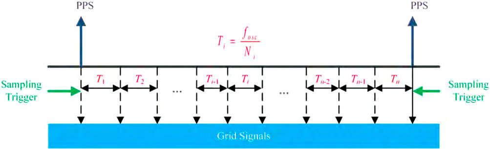
FIGURE 1. Variable sampling interval control schematic.
Adaptive synchronous sampling method mainly includes: real-time measurement of crystal output frequency, sampling control parameter adjustment, and variable sampling interval sampling. Using high-precision time pulse as a time reference to measure the crystal output frequency and trigger the first sampling command of synchronous sampling, using variable sampling interval control method, according to the real-time monitoring of the crystal output frequency to adaptively adjust the sampling control parameters, the specific steps are as follows in Figure 2.
(1) The real-time crystal output frequency ft is obtained at moment t according to Equation (4);
(2) The ideal sampling control parameter N(t) is obtained according to Equation (5);
(3) Trigger an external interrupt using a high-precision time source to trigger the first sample;
(4) Update fs and return to step 3 until sampling in one second is complete.
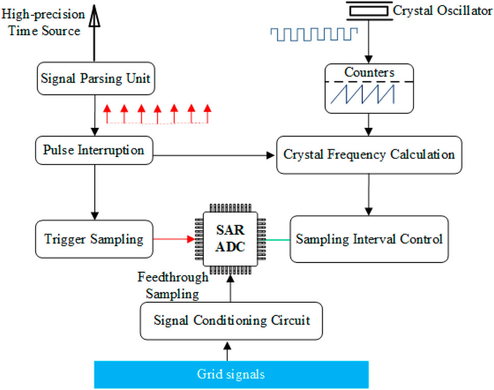
FIGURE 2. Schematic diagram of the adaptive synchronous sampling method.
Building upon the preceding section centered on high-precision pulse-sampled signals, the discrete-time signal for power system voltage or current can be expressed as follows Eq. 6:
where yk is instantaneous signal value;A is amplitude;k is sampling instant;Ti is ideal sampling time;omegais radian frequency;ϕ is phase; ɛk is additive noise(assumed to be zero-mean Gaussian white noise with variance
where
The system frequency can be found by accurately measuring the angular frequency of the voltage model in Eq. 8.
The presence of harmonics and DC attenuation distort the fundamental relationship of Equation 8 derived from the single-sine voltage signal model. n the presence of harmonics, the equation can be corrected as Eq. 9:
where m is harmonic order;M is highest frequency component of the signal; Am is amplitude of the mth harmonic; ϕm is phase of the mth harmonic.
Relationship between three consecutive samples of the corrected signal as follow Eq. 10:
If the measurement algorithm needs to be modified according to Eq. 10 in order to estimate the frequency very accurately, but in practice, the experimental results of the model given in Equation 8 are within reasonable accuracy even in the presence of harmonics.
In actual sampling, the actual sampling time Ts has time error with the ideal sampling time Ti due to the reasons such as crystal offset of the master control chipΔT.The sampling time is corrected as follows Eq. 11:
In linear systems, Kalman filters serve as indispensable tools for tracking and estimation. However, the realm of engineering practice often encounters nonlinear systems, and for such cases, the extended Kalman filter emerges as a more effective approach compared to the conventional Kalman filter. Despite numerous algorithmic advancements proposed since the 1960s to enhance the Kalman filter’s performance, tackling the estimation of state equations for nonlinear state variables remains a challenging problem, crucial for improving algorithmic accuracy. In the context of power system synchronization measurements, various state estimation methods are employed within control systems. For nonlinear state estimation, the Kalman filter is utilized as a linearized model. While it exhibits a favorable response to weakly nonlinear systems, it may fall short in accurately representing highly robust nonlinear systems. Presently, the extended Kalman filter has gained widespread adoption for tracking and state estimation. Within the Kalman filtering algorithm, predictive modeling necessitates the incorporation of actual system and process noise. Meanwhile, updating modeling involves adjusting the predicted values. Consequently, the Kalman filtering algorithm operates as a pre-calibration algorithm, encompassing time update equations (prediction equation) and measurement update equations (calibration equation), as illustrated in Figure 3.
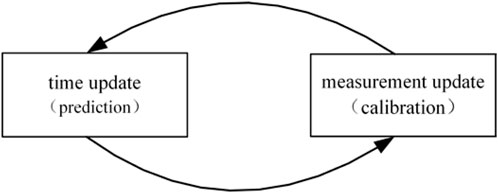
FIGURE 3. Fundamentals of the Kalman filter algorithm.
The preceding signal model satisfies the following Kalman filtered as follows Eq. 12 and as follows Eq. 13.
Based on the power system signal model, designing the ststa variable matrix shown in Eq. 14,
From the measurement equations, state equations and state variables of the system; the optimal nonlinear Kalman filtering algorithm as in Eqs 15, 16 is designed using the basic equations of Kalman filtering.
where
The optimal gain matrix is as follows Eq. 17:
The recursive equation for estimating the error variance matrix is as follows Eq. 18:
The prediction error variance can be expressed as follows Eq. 19:
where
The filter is nonlinear and therefore, the gain Kk and the covariance matrix
The problem with all Kalman filtering algorithms is resetting the covariance matrix. After initial convergence, the gain Kk and the covariance matrix Pk|k stabilise at very small values. Subsequently, when certain parameters of the signal (amplitude, phase and frequency) change, the covariance matrix must be reset to obtain a higher gain in order to track the signal quickly.
The core idea of the covariance reconstruction extended Kalman filter algorithm is that the decision to set the covariance matrix to its initial value is based on a lag-type decision block. The hysteresis band is determined by the amount of noise and the nature of convergence. If the noise estimate is about 10% of the amplitude, then the lag band is chosen to be 20%–60% of the amplitude to avoid frequent resetting of the covariance matrix. A flag is set when the error exceeds a higher threshold and reset when the error falls below a lower threshold. If the flag is 1 and either of the Kalman gains is very small, then the covariance is reset and the flag is reset to 0 so that the covariance matrix is not immediately reset.
Calculation of lag band: The hysteresis band is calculated as the ratio of the residual’s paradigm to amplitude as shown in Eq. 20:
Decide whether to set the reset flag by comparing the value of the hysteresis band with the preset threshold as shown in Eq. 21:
If the flag is 1 and either of the Kalman gains is very small, then the covariance is reset and the flag is reset to 0 so that the covariance matrix is not immediately reset as shown in Eq. 22.
Generally, the frequency variation in power systems is limited to 5 Hz. Therefore, for faster tracking, the measured frequency by the filter is not allowed to vary beyond the 40–60 Hz band. This results in stable operation of the filter and does not lead the filter wayward.
Based on the above theory, this paper constructs the dynamic synchronous phase measurement algorithm based on EKF as follows in Figure 4.
1. k = 0;
2. Project starting estimate
3. Calculate Kalman filter gain
4. Calculate the error covariance matrix Pk;
5. Determine the state estimation equationxk;
6. Predict the (k+1) th state variable
7. k = k+1;
8. Return to step (3);
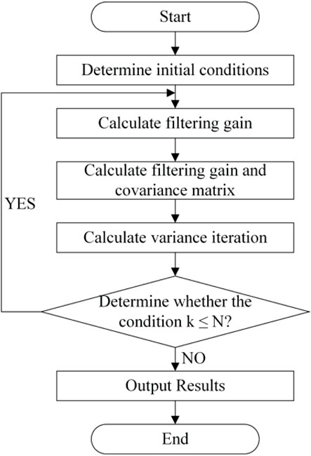
FIGURE 4. Flow chart of the extend Kalman filtering method.
The complexity analysis of the Covariance Reconstruction Extended Kalman Filter (CREKF) algorithm involves its primary steps, encompassing state prediction, state updating, covariance matrix updating, and the computation of the decision block.
The complexity analysis of the state prediction and update steps typically depends on the computational intricacy of the state and observation equations. In this paper, the equations have been linearized, resulting in a complexity denoted by O(N), where N represents the dimension of the state vector. The computation of the Kalman gain involves the Jacobian matrix of the observation equation, and thus its complexity is contingent upon the form of the observation equation, with a complexity denoted by O(N2). The complexity of the covariance matrix update is O(N3). The lagged decision block has a low complexity and consists mainly of the judgement and updating of the flags, the complexity of this step is of constant level with a complexity of O(1).
In order to verify the dynamic performance of the algorithm in this article, test signals were set up, and the simulation signals were measured and compared using the CREKF algorithm, the Recursive Discrete Fourier Transform (RDFT) algorithm, and the Matrix pencil algorithm. In this section, the measurement accuracy of the proposed algorithm is evaluated using different types of steady state and dynamic test signals according to IEC/IEEE 60255- 118-1.
The following signals are set up and the simulated signals were measured and compared by three methods. The measurement errors of the three methods are shown in Figures 5–7. Testing signal model:
a. Considering that the actual measured electrical signals contain noise, Gaussian white noise is added to the sinusoidal test signal to achieve a signal-to-noise ratio of 40 dB. The matrix beam algorithm cannot be measured accurately when the signal contains noise, so the matrix beam algorithm is not considered in the performance comparison.
b. Harmonic noise has always been a major challenge to most power system measurements. Low-order harmonics are not filtered by analog filters, and they usually appear in the waveform entering the measurement device, setting up harmonic signals.
c. During transient states, the voltage waveform of a power system may experience amplitude fluctuations of a certain Chen degree. The mathematical model of signal flicker is as
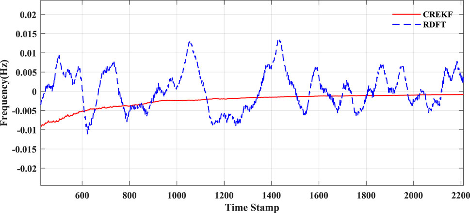
FIGURE 5. Signal contains white noise measurement results.
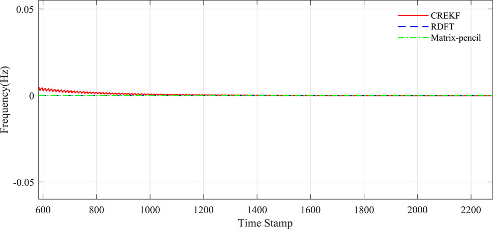
FIGURE 6. Results of the harmonic component measurements.
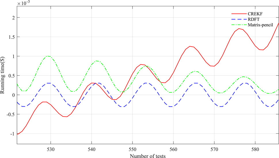
FIGURE 7. Magnitude modulation test.
The analysis of the results depicted in the figure reveals that the matrix tree algorithm encounters challenges in accurate measurements when the signal contains noise. Similarly, the recursive discrete Fourier transform demonstrates suboptimal measurement efficiency in the presence of noise. However, noteworthy is the observation that the three algorithms exhibit proximity to each other, with errors not exceeding 10–4, particularly in handling harmonic signals and flicker signals.
To further assess the dynamic tracking capability of the algorithm, a ramp signal, as defined in (Eq. 23), is employed. The algorithm’s performance is tested concerning its ability to adapt to frequency variations when the grid signal frequency undergoes gradual changes. The sampling frequency of the algorithm is fixed at fs = 1,200 Hz. Drawing from the preceding measurements’ analysis, the influence of white noise is not taken into account in the analysis of the slant wave signal.
where Rf is rate of change of frequency, set amplitude A = 1, The normal frequency of the power system is set to f = 50 Hz.
The performance comparison results of each algorithm for the above slant wave signal are shown in Figure 7.
According to the analysis of the results presented in Figure 8, the Kalman filtering algorithm demonstrates rapid tracking capabilities when the signal undergoes a sudden ramp change. In contrast, both the RDFT algorithm and the matrix-pencil algorithm exhibit difficulty accurately tracking the frequency following a recognized change in the signal’s frequency during a ramp transition.
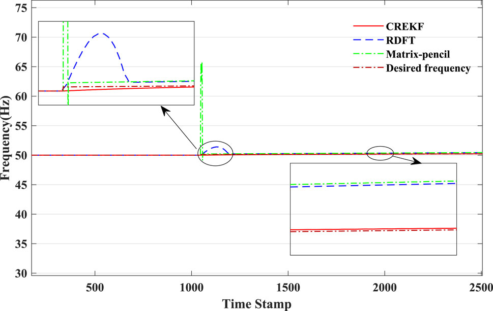
FIGURE 8. Comparison of frequency measurement results.
Utilizing the power grid signal for verification. The grid voltage signal is acquired using UGA, the sampling rate of UGA is set to 6,000 Hz and the device is shown in Figure 9. The acquired voltage signals are measured using the algorithm of this paper to verify the performance of the algorithm on a real data set.
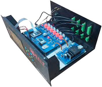
FIGURE 9. Dynamic phase measurement device.
Based on the analysis of the test results of real grid signals, the proposed algorithm can meet the standard requirements on real data sets. The test results are shown in Figure 10.
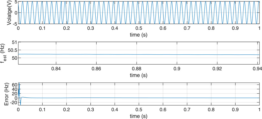
FIGURE 10. Real signal measurement results.
In terms of real-time performance, Table 1 illustrates the running time of the algorithm for each of the 10 signal calculations, comparing it with the other two algorithms. It is evident that the average processing time of the algorithm proposed in this paper is approximately 0.0189 s, significantly shorter than the processing times observed for the other two algorithms.
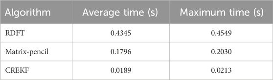
TABLE 1. Algorithm execution time comparison.
This paper explores the limitations of Kalman filtering in dealing with nonlinear systems and highlights the correlation between the algorithm’s tracking ability and the update of the covariance matrix. To this end, this paper proposes an extended Kalman filtering algorithm tailored for synchronized measurements of power system signal frequencies that contains a hysteresis band reset covariance matrix determined by the magnitude of the output error. A signal model based on high-precision time-synchronized sampling is studied in depth, and the control principle of high-precision synchronized signal sampling rate is analyzed. The dynamic characteristics of the signal are studied in depth based on the sampling data, the characteristics of the dynamic signal model are established, and the initial state of the dynamic signal of the grid is determined. Recognizing the inherent challenges of Kalman filtering in nonlinear system scenarios and acknowledging the impact of covariance matrix updating on algorithm tracking, an extended Kalman filtering algorithm is introduced in this paper. The algorithm is designed for synchronized measurements of power system signal frequencies and features a lagband reset covariance matrix, determined by the magnitude of the output error. Practical insight into power system operation guides the development of a corresponding mathematical signal model. A wide range of measurements are performed using the proposed algorithm to verify the accuracy and real-time performance of the algorithm.
1) Construct the extended Kalman filtering algorithm based on adaptive linear combiner to solve the problem that traditional Kalman filtering can not deal with nonlinear systems, and combine it with the hysteresis band updating covariance matrix which is determined by the size of the output error to improve the accuracy and real-time performance of the algorithm.
2) Measurement of various types of power system signal models. Simulation results show that for all types of mathematical signal models, the algorithm proposed in this paper has good accuracy and real-time performance, and can track the system frequency better.
The original contributions presented in the study are included in the article/supplementary material, further inquiries can be directed to the corresponding author.
JZ: Writing–original draft. FL: ZC: CH: CL: ST: Writing–review and editing.
The author(s) declare financial support was received for the research, authorship, and/or publication of this article. This work was funded by the Science and Technology Project of State Grid Co., LTD. Project Name: Research on key technologies and prototype development based on timing pulse characteristics of 5G communication network (No. 52199723008).
Authors JZ and FL were employed by State Grid Sichuan Electric Power Company Electric Power Science Research Institute. Author CH was employed by Neijiang Power Supply Company of State Grid Sichuan Electric Power Company. Author CL was employed by Leshan Power Supply Company of State Grid Sichuan Electric Power Company.
The remaining author declares that the research was conducted in the absence of any commercial or financial relationships that could be construed as a potential conflict of interest.
All claims expressed in this article are solely those of the authors and do not necessarily represent those of their affiliated organizations, or those of the publisher, the editors and the reviewers. Any product that may be evaluated in this article, or claim that may be made by its manufacturer, is not guaranteed or endorsed by the publisher.
Aminifar, F., Shahidehpour, M., Fotuhi-Firuzabad, M., and Kamalinia, S. (2013). Power system dynamic state estimation with synchronized phasor measurements. IEEE Trans. Instrum. Meas. 63, 352–363. doi:10.1109/tim.2013.2278595
Amirat, Y., Oubrahim, Z., Ahmed, H., Benbouzid, M., and Wang, T. (2020). Phasor estimation for grid power monitoring: least square vs linear kalman filter. Energies 13, 2456. doi:10.3390/en13102456
Bashian, A., Macii, D., Fontanelli, D., and Petri, D. (2021). “Kalman filtering with harmonics whitening for p class phasor measurement units,” in 2021 IEEE 11th International Workshop on Applied Measurements for Power Systems (AMPS), Cagliari, Italy, 29 September 2021 - 01 October 2021 (IEEE), 1–6.
bin Mohd Nasir, M. N., Sabo, A., and Wahab, N. I. A. (2019). “A review on synchrophasor technology for power system monitoring,” in 2019 IEEE student conference on research and development (SCOReD) (IEEE), Seri Iskandar, Perak, Malaysia, October 15-17, 2019, 58–62.
Dash, P., Krishnanand, K., and Patnaik, R. (2013). Dynamic phasor and frequency estimation of time-varying power system signals. Int. J. Electr. Power and Energy Syst. 44, 971–980. doi:10.1016/j.ijepes.2012.08.063
de la O Serna, J. A., Paternina, M. A., and Zamora-Mendez, A. (2020). Assessing synchrophasor estimates of an event captured by a phasor measurement unit. IEEE Trans. Power Deliv. 36, 3109–3117. doi:10.1109/tpwrd.2020.3033755
Fan, L. (2015). “Least squares estimation and kalman filter based dynamic state and parameter estimation,” in 2015 IEEE Power and Energy Society General Meeting (IEEE), Denver, Colorado, USA, 26-30 July 2015, 1–5.
Fan, L., and Wehbe, Y. (2013). Extended kalman filtering based real-time dynamic state and parameter estimation using pmu data. Electr. Power Syst. Res. 103, 168–177. doi:10.1016/j.epsr.2013.05.016
Ferrero, R., Pegoraro, P. A., and Toscani, S. (2019). Dynamic synchrophasor estimation by extended kalman filter. IEEE Trans. Instrum. Meas. 69, 4818–4826. doi:10.1109/tim.2019.2955797
Ferrero, R., Pegoraro, P. A., and Toscani, S. (2020). Synchrophasor estimation for three-phase systems based on taylor extended kalman filtering. IEEE Trans. Instrum. Meas. 69, 6723–6730. doi:10.1109/tim.2020.2983622
Hou, R., Wu, J., Song, H., Qu, Y., and Xu, D. (2020). Applying directly modified rdft method in active power filter for the power quality improvement of the weak power grid. Energies 13, 4884. doi:10.3390/en13184884
Huang, C., Xie, X., and Jiang, H. (2017). Dynamic phasor estimation through dstkf under transient conditions. IEEE Trans. Instrum. Meas. 66, 2929–2936. doi:10.1109/tim.2017.2713018
Khodaparast, J. (2022). A review of dynamic phasor estimation by non-linear kalman filters. IEEE Access 10, 11090–11109. doi:10.1109/access.2022.3146732
Khodaparast, J., and Khederzadeh, M. (2017). Least square and kalman based methods for dynamic phasor estimation: a review. Prot. Control Mod. Power Syst. 2, 1–18. doi:10.1186/s41601-016-0032-y
Liu, H., Hu, F., Su, J., Wei, X., and Qin, R. (2020). Comparisons on kalman-filter-based dynamic state estimation algorithms of power systems. Ieee Access 8, 51035–51043. doi:10.1109/access.2020.2979735
Liu, J., Ni, F., Tang, J., Ponci, F., and Monti, A. (2012). “A modified taylor-kalman filter for instantaneous dynamic phasor estimation,” in 2012 3rd IEEE PES Innovative Smart Grid Technologies Europe (ISGT Europe) (IEEE), Berlin, Germany, 14-17 October 2012, 1–7.
Mai, R. K., Fu, L., Dong, Z. Y., Kirby, B., and Bo, Z. Q. (2011). An adaptive dynamic phasor estimator considering dc offset for pmu applications. IEEE Trans. Power Deliv. 26, 1744–1754. doi:10.1109/tpwrd.2011.2119334
Mohanty, M., Kant, R., Kumar, A., Sahu, D., and Choudhury, S. (2020). A brief review on synchro phasor technology and phasor measurement unit. Adv. Electr. Control Signal Syst. Sel. Proc. AECSS 2019, 705–721. doi:10.1007/978-981-15-5262-5_53
Song, J., Zhang, J., and Wen, H. (2021). Accurate dynamic phasor estimation by matrix pencil and taylor weighted least squares method. IEEE Trans. Instrum. Meas. 70, 1–11. doi:10.1109/tim.2021.3066187
Wang, M., and Sun, Y. (2004). A practical, precise method for frequency tracking and phasor estimation. IEEE Trans. power Deliv. 19, 1547–1552. doi:10.1109/tpwrd.2003.822544
Xiao, H., Gan, H., Yang, P., Li, L., Li, D., Hao, Q., et al. (2023). Robust submodule fault management in modular multilevel converters with nearest level modulation for uninterrupted power transmission. IEEE Trans. Power Deliv., 1–16. doi:10.1109/TPWRD.2023.3343693
Xiao, H., He, H., Zhang, L., and Liu, T. (2023). Adaptive grid-synchronization based grid-forming control for voltage source converters. IEEE Trans. Power Syst. 1, 1–4. doi:10.1109/TPWRS.2023.3338967
Keywords: highly accurate synchronized time source, adaptive sampling rate, dynamic phasor measurement, Kalman filter, reconstructing the covariance equation
Citation: Zhang J, Li F, Chang Z, Hu C, Liu C and Tang S (2024) Dynamic phasor measurement algorithm based on high-precision time synchronization. Front. Sig. Proc. 4:1357995. doi: 10.3389/frsip.2024.1357995
Received: 19 December 2023; Accepted: 13 February 2024;
Published: 29 February 2024.
Edited by:
Tao Peng, Soochow University, ChinaReviewed by:
Mehdi Korki, Swinburne University of Technology, AustraliaCopyright © 2024 Zhang, Li, Chang, Hu, Liu and Tang. This is an open-access article distributed under the terms of the Creative Commons Attribution License (CC BY). The use, distribution or reproduction in other forums is permitted, provided the original author(s) and the copyright owner(s) are credited and that the original publication in this journal is cited, in accordance with accepted academic practice. No use, distribution or reproduction is permitted which does not comply with these terms.
*Correspondence: Sihao Tang, dGFuZ3NpaGFvQGhudS5lZHUuY24=
Disclaimer: All claims expressed in this article are solely those of the authors and do not necessarily represent those of their affiliated organizations, or those of the publisher, the editors and the reviewers. Any product that may be evaluated in this article or claim that may be made by its manufacturer is not guaranteed or endorsed by the publisher.
Research integrity at Frontiers
Learn more about the work of our research integrity team to safeguard the quality of each article we publish.