Bayesian learning of nonlinear gene regulatory networks with switching architectures

Introduction: Gene regulatory networks (GRNs) are characterized by their dynamism, meaning that the regulatory interactions which constitute these networks evolve with time. Identifying when changes in the GRN architecture occur can inform our understanding of fundamental biological processes, such as disease manifestation, development, and evolution. However, it is usually not possible to know a priori when a change in the network architecture will occur. Furthermore, an architectural shift may alter the underlying noise characteristics, such as the process noise covariance.

Methods: We develop a fully Bayesian hierarchical model to address the following: a) sudden changes in the network architecture; b) unknown process noise covariance which may change along with the network structure; and c) unknown measurement noise covariance. We exploit the use of conjugate priors to develop an analytically tractable inference scheme using Bayesian sequential Monte Carlo (SMC) with a local Gibbs sampler.

Results: Our Bayesian learning algorithm effectively estimates time-varying gene expression levels and architectural model indicators under varying noise conditions. It accurately captures sudden changes in network architecture and accounts for time-evolving process and measurement noise characteristics. Our algorithm performs well even under high noise conditions. By incorporating conjugate priors, we achieve analytical tractability, enabling robust inference despite the inherent complexities of the system. Furthermore, our method outperforms the standard particle filter in all test scenarios.

Discussion: The results underscore our method’s efficacy in capturing architectural changes in GRNs. Its ability to adapt to a range of time-evolving noise conditions emphasizes its practical relevance for real-world biological data, where noise presents a significant challenge. Overall, our method provides a powerful tool for studying the dynamics of GRNs and has the potential to advance our understanding of fundamental biological processes.

1 Introduction

Gene regulatory networks (GRNs) are complex systems consisting of genes and a toolkit of molecular elements responsible for coordinating the spatiotemporal allocation of gene expression in every cell of the body. They are involved in the execution of essential biological processes, such as development, metabolism, and responses to environmental signals. One of their key characteristics is dynamicity. The regulatory interactions constituting these networks are not static; rather, they evolve, giving rise to time-dependent GRN architectures. These temporal alterations in regulatory structures have consequences for the biological processes which are encoded by GRNs across both short and long time scales and can affect all major biological processes, including development, disease, and phenotypic evolution. GRNs also exhibit a complex hierarchical architecture comprised of interlinked subunits called “subcircuits.” Ranging from two to eight genes, these subcircuits consist of specific regulatory interactions that execute specific biological functions (Peter and Davidson, 2011). Subcircuits thus intimately link structure and function GRNs (Hinman and Cheatle Jarvela, 2014). Research shows that these subcircuits are evolutionarily conserved across Metazoa, reinforcing their critical role (Peter and Davidson, 2015). Various subcircuit types, such as positive-feedback loops, feed-forward connections, and reciprocal repression mechanisms, have been identified (Alon, 2019). During development, different subcircuits are involved in different temporal stages of the developmental process, such as pattern formation, state stabilization, and cellular differentiation (Peter and Davidson, 2015). As development proceeds, the sets of active genes and their associated regulatory interactions change. In regard to disease, the rewiring of regulatory networks can cause disruptions in essential biological functions, giving rise to diseases such as cancer or disorders such as schizophrenia (Potkin et al., 2010). These rewirings can manifest at the level of subcircuits, which emphasizes their importance in understanding disease mechanisms (Saunders and McClay, 2014). Such alterations may involve transitions from one subcircuit type to another—for example, a shift from a positive-feedback loop to a feed forward cascade (Saunders and McClay, 2014). Similarly, evolutionary changes in GRN configurations contribute to the emergence of novel phenotypes within populations (Ha et al., 2022). Identifying these shifts in GRN interactions, especially within subcircuits, is thus an imperative task for understanding essential biological processes. This is fundamentally a change point detection problem.

To this extent, state-space models provide a mathematical framework that captures the dynamical behavior of GRNs, including their subcircuits, over time. GRN estimation using a state space approach has been extensively studied (Noor et al., 2012; Bugallo et al., 2015; Ancherbak et al., 2016; Pirgazi and Khanteymoori, 2018; Amor et al., 2019). However, these approaches assume that the network structure is static across all time. To this extent, several works have considered the problem of estimating GRNs with time-varying structures using linear models. Specifically, the authors in (Xiong and Zhou, 2013; Pirgazi and Khanteymoori, 2018) use Kalman filtering for inference by assuming a linear state-space model. In (Noor et al., 2012; Bugallo et al., 2015; Ancherbak et al., 2016), particle filtering is used to infer the dynamic network and the process and measurement noise are assumed to be known and constant. This may not capture changes in the noise statistics that can arise when a change in the regulatory network structure occurs. In (Dondelinger et al., 2013), the network structure assumed to change slowly across time. However, environmental stressors, disease, or mutations may substantially alter the network structure in a more abrupt manner. Furthermore, gene regulation is a nonlinear process due to the feedback loops present in the architectures, threshold effects, and combinatorial binding of transcription factors on DNA. Linear models may therefore obscure these phenomena. Alternatively, nonlinear system models based on Hill kinetics, Michaelis-Menten kinetics, or the S-system are able to more accurately capture the molecular mechanisms of gene regulation (Wang et al., 2007; Youseph et al., 2015; 2019; Elahi and Hasan, 2018). Nonlinear Bayesian filtering inference methods, such as extended Kalman filtering and particle filtering, were used with these nonlinear models (Wang et al., 2009; Zhang et al., 2014; Bugallo et al., 2015). In (Lee et al., 2013), a nonlinear chemical kinetics model is considered, but the transition probabilities for switching between various network structures (or modes) are assumed to be known, which is usually not the case in practice.

Given the limitations of these works, we propose a fully Bayesian hierarchical model with sequential learning to account for the following: (a) sudden changes in the network architecture, (b) unknown modeling error process covariance, and (c) unknown measurement noise covariance. Using Bayesian hierarchical modeling allows for uncertainty at all levels and the use of prior information and inference techniques. It can also be integrated with sequential Monte Carlo (SMC) methods, offering the ability to handle nonlinear and non-Gaussian processes, which are often the case in biological systems. Within this framework, we use Bayesian learning for the predictive modeling of dynamic transitions between GRN subcircuits. This approach not only allows us to build upon existing domain knowledge but also to develop models with the complexity necessary for identifying temporal changes in the GRN interactions. In our model, the regulatory network interactions are encoded by kinetic order parameters, which we assume change at unknown times. Our proposed method exploits the use of conjugate priors to enable tractable and efficient inference and SMC with local Gibbs sampling Gelfand et al. (1990); Gelman et al. (1995) to choose among the network configurations and estimate the model and trajectories of the gene expression values.

This paper is organized as follows. In Section 2.1, we review the dynamic nonlinear state space model for GRNs and extend it to allow for time-variations in the direction and type of gene regulation in Section 2.2. In Section 2.3, we present our proposed approach to learning time-variations in GRNs; and in Section 2.4, we discuss our implementation using SMC inference with local Gibbs sampling. Simulations are presented in Section 3 to demonstrate the efficacy of our Bayesian hierarchical learning and tracking.

2 Materials and methods

2.1 Modeling gene regulatory networks

In (Vélez-Cruz et al., 2021), we developed a stochastic nonlinear GRN model to capture the molecular mechanisms of gene regulation and account for inherent variability in biological processes. The model includes information on binding affinity, expression and self-decay rates. It is based on Michaelis-Menten kinetics that describe different types of regulation processes between a gene and multiple other genes (Youseph et al., 2015; Youseph et al., 2019; Krishnan et al., 2020). It also incorporates the Hill coefficient that represents the effect of binding affinity between genes (Alon, 2019). We represent the GRN model by a dynamics state space formulation for N genes X_i, i = 1, …, N as.

${\mathbf{x}}_k=\mathit{\varphi }\left({\mathbf{x}}_{k-1}\right)+{\mathbf{w}}_{k-1}(1)$

${\mathbf{y}}_k={\mathbf{x}}_k+{\mathbf{v}}_k(2)$

Where ${\mathbf{x}}_k={[x_{1,k}\dots x_{N,k}]}^T$, x_i,k, i = 1, …, N, is the expression level of Gene i at time step k, ${\mathbf{y}}_k={[y_{1,k}\dots y_{N,k}]}^T$, y_i,k is the microarray measurement for Gene X_i, w_k is measurement noise, and v_k is a random process used to represent modeling error uncertainty. In Eq. 1, the ith element of the N × 1 transition vector ϕ(x_k−1) is given by

${\left[\mathit{\varphi }\left({\mathbf{x}}_{k-1}\right)\right]}_i={\left[\mathit{\rho }\left({\mathbf{x}}_{k-1}\right)\right]}_i-\sigma \left(x_{i,k-1}\right)={\left[\mathit{\psi }\left({\mathbf{x}}_{k-1}\right)\right]}_i{\displaystyle \prod _{\begin{array}{c}j=1\\ j\ne i\end{array}}^N}{\mathbf{a}}_{ij}{\mathbf{b}}_{ij}\left({\mathbf{x}}_{k-1}\right)-v_i^d{x}_{i,k-1}(3)$

where the terms ${[\mathit{\rho }({\mathbf{x}}_{k-1})]}_i$ and σ(x_i,k−1) denote production and degradation, respectively, $v_i^d$ is the self-decay rate of protein or mRNA expressed by Gene X_i.

${\left[\mathit{\psi }\left({\mathbf{x}}_{k-1}\right)\right]}_i=\frac{v_i^{\max }}{\left(K_{ii}^{q_{ii}}+x_{i,k-1}^{q_{ii}}\right){\prod }_{\begin{array}{c}j=1\\ j\ne i\end{array}}^N\left(K_{ij}^{q_{ij}}+x_{j,k-1}^{q_{ij}}\right)}(4)$

${\mathbf{a}}_{ij}=\left[\begin{array}{cccc}\hfill g_{ii}{g}_{ij}\hfill & \hfill g_{ii}{h}_{ij}\hfill & \hfill h_{ii}{g}_{ij}\hfill & \hfill h_{ii}{h}_{ij}\hfill \end{array}\right](5)$

${\mathbf{b}}_{ij}\left({\mathbf{x}}_{k-1}\right)={\left[\begin{array}{cccc}\hfill x_{i,k-1}^{q_{ii}}{x}_{j,k-1}^{q_{ij}}\hfill & \hfill x_{i,k-1}^{q_{ii}}{K}_{ij}^{q_{ij}}\hfill & \hfill x_{j,k-1}^{q_{12}}{K}_{ii}^{q_{ii}}\hfill & \hfill K_{ii}^{q_{ii}}{K}_{ij}^{q_{ij}}\hfill \end{array}\right]}^T,(6)$

And $v_i^{\max }$ is the maximum expression rate of Gene X_i.

All model parameters are described in Table 1. We specifically note the following parameters for Gene X_i and Gene X_j, i ≠ j. The Hill coefficient q_ij in Eq. 4 represents how the binding affinity of X_j increases the binding affinity of X_i. The Michaelis-Menten constant K_ij accounts for the binding affinity between the product of X_j and the binding site of a target X_i; large values of K_ij indicate a low binding affinity. The kinetic order parameters h_ij and g_ij in Eq. 5 take values of 0 or 1. Different combinations of these parameters indicate the type of regulation, as summarized in Table 2. Note that parameters K_ii, q_ii, h_ii and g_ii specify autoregulatory interactions.

Table 1

Table 1. Definition of GRN state-space model parameters in Eq. 1 and Eq. 2.

Table 2

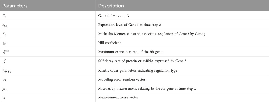
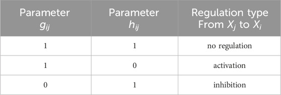
Table 2. GRN kinetic order parameters indicating type of regulation from Gene X_j to Gene X_i, i = j; autoregulation is indicated by g_ii = h_ii = 1.

2.2 Formulation of time-varying GRN model

We consider a TV GRN model where both the direction and type of regulation vary with time. This time variation is reflected in the kinetic order parameters in Eq. 5.

${\mathbf{a}}_{ij,k}=\left[g_{ii,k}{g}_{ij,k}{g}_{ii,k}{h}_{ij,k}{h}_{ii,k}{g}_{ij,k}{h}_{ii,k}{h}_{ij,k}\right],(7)$

and thus in the transition function ϕ_k (⋅) in Eqs. (1) and (3). With this TV model, we can describe interactions between any number of genes and capture any changes in the GRN configuration with varying degrees of complexity.

As a simple illustration, we consider the transition from time step k − 1 to k of the simple GRN in Figure 1A to the one in Figure 1B. In Figure 1A, Genes X₁ and X₂ activate each other’s expression in a positive feedback loop at k − 1. From Table 2, activation of Gene X₁ by Gene X₂ is indicated by h₁₂ = 0 and g₁₂ = 1 and activation of Gene X₂ by Gene X₁ is indicated by h₂₁ = 0 and g₂₁ = 1. Thus, the kinetic order parameter vector at time step k − 1 is given by

$\begin{array}{ccc}\hfill & \hfill & {\mathbf{a}}_{12,k-1}={\mathbf{a}}_{X_1\leftarrow X_2,k-1}=\left[g_{11,k-1}{g}_{12,k-1}{g}_{11,k-1}{h}_{12,k-1}{h}_{11,k-1}{g}_{12,k-1}{h}_{11,k-1}{h}_{12,k-1}\right]\hfill \\ \hfill & \hfill & =\left[01000100\right]={\mathbf{a}}_{X_2\leftarrow X_1,k-1}={\mathbf{a}}_{21,k-1}.\hfill \end{array}$

where notation X₁ ← X₂ denotes the interaction from Gene X₂ to Gene X₁. In Figure 1B, the interaction from Gene X₂ to Gene X₁ switches from activation to inhibitory at time k. Whereas a_21,k = a_21,k−1, since inhibition of Gene X₁ by Gene X₂ is indicated by h₁₂ = 1 and g₁₂ = 0, then

${\mathbf{a}}_{X_1\leftarrow X_2,k}=\left[g_{11,k}{g}_{12,k}{g}_{11,k}{h}_{12,k}{h}_{11,k}{g}_{12,k}{h}_{11,k}{h}_{12,k}\right]=\left[00010001\right]$

Figure 1

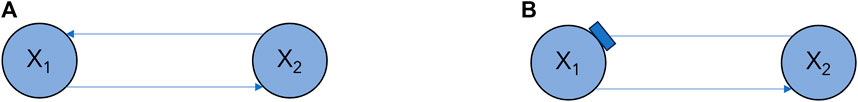
Figure 1. Simple feedback loops demonstrating different types of regulatory interactions: (A) Gene X₁ activates the expression of gene X₂ and gene X₂ activates the expression of gene X₁. (B) Gene X₁ activates the expression of gene X₂ and gene X₂ inhibits the expression of gene X₁. The arrows denote activating regulatory interactions, whereas the line with the vertical bar denotes an inhibitory regulatory interaction.

For a realistic scenario, we consider the transcriptional activator Gcn4 of several amino acid biosynthesis genes in Saccharomyces cerevisiae or yeast (Mittal et al., 2017) and the transcription factor LexA responsible for repressing several genes involved in DNA repair in bacteria (McKenzie et al., 2000). Under stressful conditions such as nutrient deprivation, the network may switch from a single-input module configuration to a state which requires the coordination between several genes such as in a feed forward loop. For N = 5 genes, this configuration switch is depicted as changing from the subcircuit in Figure 2A to the subcircuit in Figure 2B. For example, when yeast are subject to osmotic stress, the high-osmolarity glycerol pathway is activated; this involves the subsequent activation of several genes involved in metabolism regulation, temporary arrest of cell cycle progression, or many other processes that are required for cellular adaptation in a feed forward architecture (Nadal and Posas, 2022). More complex subcircuits are found, for example, in the hypothalamic-pituitary-adrenal axis, which is responsible for regulating the stress response in humans (Tsigos and Chrousos, 2002).

Figure 2

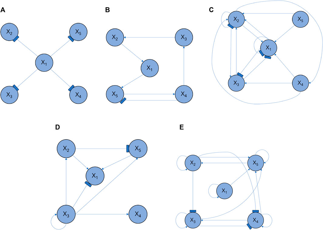
Figure 2. GRN subcircuit models in Section 3.1: (A) M₁, (B) M₂, (C) M₃, (D) M₄, (E) M₅.

2.3 Bayesian learning for tracking

In this paper, we propose a new method for estimating the TV gene expressions under the realistic conditions of sudden changes in the GRN architecture and unknown statistics in the state space formulation. In particular, we assume that the GRN circuit features on developmental function can be selected from M subcircuit models. The mth model at time step k, denoted by the indicator s_k = m, m = 1, …, M, is associated with the mth TV kinematic order parameter vector ${\mathbf{a}}_{ij,k}^{(m)}={\mathbf{a}}_{ij,k}$ in Eq. 7. The state space formulation for estimating x_k is now given by.

${\mathbf{x}}_k=\mathit{\varphi }\left({\mathbf{x}}_{k-1},s_k=m\right)+{\mathbf{w}}_{k-1}^{\left(m\right)}(8)$

${\mathbf{y}}_k={\mathbf{x}}_k+{\mathbf{v}}_k,(9)$

Where the modeling error process ${\mathbf{w}}_{k-1}^{(m)}\sim \mathcal{N}(\mathbf{0},{\mathrm{\Sigma }}_{\mathbf{w}}^{(m)})$ for the mth model and the measurement noise ${\mathbf{v}}_k\sim \mathcal{N}(\mathbf{0},{\mathrm{\Sigma }}_{\mathbf{v}})$ are both assumed zero-mean Gaussian with constant but unknown covariance matrices ${\mathrm{\Sigma }}_{\mathbf{w}}^{(m)}$ and Σ_v, respectively.

The new method, Bayesian Learning for Tracking or BLT, sequentially estimates the gene expressions while learning the probability of selecting one of the M models at each time step k as well as the unknown covariance matrices. From Eq. 8, the model indicator is drawn from a categorical distribution with parameter vector ${\mathit{\pi }}_k=[{\pi }_k^{(1)}\dots {\pi }_k^{(M)}]$; specifically, s_k ∣ π_k, M ∼Cat(s_k ∣ π_k, M), where ${\pi }_k^{(m)}=\text{Pr}(s_k=m)$ is the probability of selecting the mth model at time k and π ∣ α ∼ Dir(α) is obtained from a Dirichlet distribution prior with concentration hyperparameter α = [α₁, …, α_M] (Sudderth, 2016). The prior probability that the existing model m is selected at time step k is

$p\left(s_k=m\mid {\mathcal{S}}_{k-1},{\pi }_k^{\left(m\right)},{\alpha }_m\right)=\frac{c_{1:k-1}^{\left(m\right)}}{{\displaystyle \sum _{l=1}^m}{c}_{1:k-1}^{\left(l\right)}+{\alpha }_m}(10)$

where ${\mathcal{S}}_{k-1}=\{s_1,\dots ,s_{k-1}\}$ and $c_{1:k-1}^{(m)}$ is the number of times the mth model was selected up to the previous time step k − 1. The covariance matrix ${\mathrm{\Sigma }}_{\mathbf{w}}^{(m)}\mid {\mathbf{\Psi }}_{\mathbf{w}}^{(m)}\sim \text{IWD}({\mathbf{\Psi }}_{\mathbf{w}}^{(m)})$ is modeled using an inverse Wishart distribution (IWD) prior with hyperparameter ${\mathbf{\Psi }}_{\mathbf{w}}^{(m)}=\{{\mathrm{\Lambda }}_{\mathbf{w}}^{(m)},{\nu }_{\mathbf{w}}^{(m)}\}$. Here, ${\mathrm{\Lambda }}_{\mathbf{w}}^{(m)}$ is the scale matrix and ${\nu }_{\mathbf{w}}^{(m)}$ is the number of degrees of freedom (Gelman et al., 1995).

The overall learning model is summarized by the following hierarchy

$\begin{array}{ccc}\hfill & \hfill & {\mathbf{x}}_k\mid {\mathbf{x}}_{k-1},s_k=m,{\mathrm{\Sigma }}_{\mathbf{w}}^{\left(m\right)}\sim \mathcal{N}\left(\cdot \mid {\mathbf{x}}_{k-1},s_k=m,{\mathrm{\Sigma }}_{\mathbf{w}}^{\left(m\right)}\right)\hfill \\ \hfill & \hfill & {\mathbf{y}}_k\mid {\mathbf{x}}_k,{\mathrm{\Sigma }}_{\mathbf{v}}\sim \mathcal{N}\left(\cdot \mid {\mathbf{x}}_k,{\mathrm{\Sigma }}_{\mathbf{v}}\right)\hfill \\ \hfill & \hfill & s_k\mid {\mathcal{S}}_{k-1},{\pi }_k^{\left(m\right)},{\alpha }_m\sim \text{Cat}\left({\mathit{\pi }}_k,M\right)\hfill \\ \hfill & \hfill & {\pi }_k^{\left(m\right)}\mid {\alpha }_m\sim \text{Dir}\left(\mathit{\alpha }\right)\hfill \\ \hfill & \hfill & {\mathrm{\Sigma }}_{\mathbf{w}}^{\left(m\right)}\mid {\mathbf{\Psi }}_{\mathbf{w}}^{\left(m\right)}\sim \text{IWD}\left({\mathbf{\Psi }}_{\mathbf{w}}^{\left(m\right)}\right)\hfill \\ \hfill & \hfill & {\mathrm{\Sigma }}_{\mathbf{v}}\mid {\mathbf{\Psi }}_{\mathbf{v}}\sim \text{IWD}\left({\mathbf{\Psi }}_{\mathbf{v}}\right).\hfill \end{array}$

Following a sequential Bayesian Monte Carlo approach, the model first predicts x_k using

$\begin{array}{ccc}\hfill & \hfill & p\left({\mathbf{x}}_k\mid {\mathbf{x}}_{k-1},s_k=m,{\mathcal{S}}_{k-1},{\pi }_k^{\left(m\right)},{\alpha }_m,{\mathrm{\Sigma }}_{\mathbf{w}}^{\left(m\right)},{\mathbf{\Psi }}_{\mathbf{w}}^{\left(m\right)}\right)\propto \hfill \\ \hfill & \hfill & p\left({\mathbf{x}}_k\mid {\mathbf{x}}_{k-1},s_k=m,{\mathrm{\Sigma }}_{\mathbf{w}}^{\left(m\right)}\right)p\left(s_k=m\mid {\mathcal{S}}_{k-1},{\pi }_k^{\left(m\right)},{\alpha }_m\right)p\left({\pi }_k^{\left(m\right)}\mid {\alpha }_m\right)p\left({\mathrm{\Sigma }}_{\mathbf{w}}^{\left(m\right)}\mid {\mathbf{\Psi }}_{\mathbf{w}}^{\left(m\right)}\right)\hfill \end{array}(11)$

where $p({\mathbf{x}}_k\mid {\mathbf{x}}_{k-1},s_k=m,{\mathrm{\Sigma }}_{\mathbf{w}}^{(m)})$ is obtained from Eq. 8, $p(s_k=m\mid {\mathcal{S}}_{k-1},{\pi }_k^{(m)},{\alpha }_m)$ is the categorical distribution in Eq. 10, $p({\pi }_k^{(m)}\mid {\alpha }_m)$ is the Dirichlet prior, and $p({\mathrm{\Sigma }}_{\mathbf{w}}^{(m)}\mid {\mathbf{\Psi }}_{\mathbf{w}}^{(m)})$ is the IWD prior.

Before using measurement y_k to update the state x_k at time step k, the noise covariance matrix Σ_v ∼IWD (Ψ_v) is learned using an IWD prior with hyperparameter Ψ_v = {Λ_v, ν_v}. This results in

$p\left({\mathbf{y}}_k\mid {\mathbf{x}}_k,{\mathrm{\Sigma }}_{\mathbf{v}},{\mathbf{\Psi }}_{\mathbf{v}}\right)\propto p\left({\mathbf{y}}_k\mid {\mathbf{x}}_k,{\mathrm{\Sigma }}_{\mathbf{v}}\right)p\left({\mathrm{\Sigma }}_{\mathbf{v}}\mid {\mathbf{\Psi }}_{\mathbf{v}}\right)(12)$

where p (y_k ∣ x_k, Σ_v) is given in Eq. 9 and p (Σ_v ∣ Ψ_v) is the IWD prior. Using Eqs. (11) and (12), the joint posterior distribution at each time step k is given by

$\begin{array}{ccc}\hfill & \hfill & p\left({\mathbf{x}}_k,s_k=m,{\pi }_k^{\left(m\right)},{\mathrm{\Sigma }}_{\mathbf{w}}^{\left(m\right)},{\mathrm{\Sigma }}_{\mathbf{v}}\mid {\mathbf{y}}_k,{\mathcal{S}}_{k-1},{\alpha }_m,{\mathbf{\Psi }}_{\mathbf{w}}^{\left(m\right)},{\mathbf{\Psi }}_{\mathbf{v}}\right)\propto \hfill \\ \hfill & \hfill & p\left({\mathbf{x}}_k\mid {\mathbf{x}}_{k-1},s_k=m,{\mathcal{S}}_{k-1},{\pi }_k^{\left(m\right)},{\alpha }_m,{\mathrm{\Sigma }}_{\mathbf{w}}^{\left(m\right)},{\mathbf{\Psi }}_{\mathbf{w}}^{\left(m\right)}\right)p\left({\mathbf{y}}_k\mid {\mathbf{x}}_k,{\mathrm{\Sigma }}_{\mathbf{v}},{\mathbf{\Psi }}_{\mathbf{v}}\right)\hfill \\ \hfill & \hfill & p\left({\mathbf{x}}_{k-1},s_{k-1},{\pi }_{k-1}^{s_{k-1}},{\mathrm{\Sigma }}_{\mathbf{w}}^{\left(s_{k-1}\right)},{\mathrm{\Sigma }}_{\mathbf{v}}\mid {\mathbf{y}}_{k-1},{\alpha }_{s_{k-1}},{\mathbf{\Psi }}_{\mathbf{w},\text{prev}}^{\left(s_{k-1}\right)},{\mathbf{\Psi }}_{\mathbf{v},\text{prev}}\right).\hfill \end{array}(13)$

The last distribution in Eq. 13 is the posterior from the previous time step, obtained using model s_k−1, where ${\mathbf{\Psi }}_{\mathbf{w},\text{prev}}^{(s_{k-1})}$ and Ψ_v,prev are the IWD hyperparameters used at time step k − 1.

Note that the derivation of the BLT is provided in Supplementary Appendix A.

2.4 BLT implementation using particle filtering and local Gibbs sampling

The dynamic state space model in Eqs. (1)-(6) is highly nonlinear, so we implement the BLT using particle filtering (Arulampalam et al., 2002; Elvira et al., 2019). As Eq. 11 is not explicitly known, the PF also estimates both the unknown TV model indicator s_k and unknown constant covariance matrix ${\mathrm{\Sigma }}_{\mathbf{w}}^{(s_k)}$. However, the PF performs poorly when used to estimate parameters that do not change with time (Chopin, 2002). One approach to improve the PF performance for constant parameters, MCMC can be used together with a rejuvenation test based on the Kullback–Leibler divergence measure (Lee and Chia, 2002; Li and Papandreou-Suppappola, 2006). For the BLT, we instead use local Gibbs sampling (Gelfand et al., 1990; Gelman et al., 1995; Martino et al., 2018) at each time step k in order to sample from available multivariate conditional distributions and sequentially update the constant IWD hyperparameters of the covariance matrix.

The BLT implementation steps are summarized in Algorithm 1. The algorithm uses the joint prior in Eq. 11 as the PF proposal distribution and assumes N_s state particles. At each time step and particle, we perform L Gibbs sampling iterations. In what follows, ${\mathbf{x}}_{i,k}^{(\ell )}$ denotes the ith particle, i = 1, …, N_s, at the ℓth iteration, ℓ = 0, …L, at time step k; similarly, $s_{i,k}^{(\ell )}$ denotes the model indicator, ${\pi }_{i,k}^{(m,\ell )}$ denotes the probability of the mth model, m = 1, …, M, $c_{i,1:k-1}^{(m,\ell )}$ denotes the number of times the mth model is selected up to time step k − 1, and ${\mathrm{\Sigma }}_{\mathbf{w},i}^{(m,\ell )}$ denotes the mth modeling error covariance matrix. At ℓ = 0, the iterations are initialized using the estimates obtained from the previous time step, ${\mathbf{x}}_{i,k}^{(0)}={\mathbf{x}}_{i,k-1}$ and ${\mathrm{\Sigma }}_{\mathbf{w},i}^{(m,0)}={\mathrm{\Sigma }}_{\mathbf{w},i}^{(s_{i,k-1})}$. At the ℓth iteration, ℓ = 1, …, L, the algorithm.

Algorithm 1.Sequential Monte Carlo with Local Gibbs Sampling for Subcircuit Detection.

1: Initialization at t = 1

2: for i = 1, …, N particles do

3: Sample ${\mathbf{x}}_1^{(i)}\sim p({\mathbf{x}}_1)$

4: Sample $s_1^{(i)}\sim \text{Cat}({\mathit{\pi }}_1)$

5: Sample ${\{{\mathrm{\Sigma }}_w^{m,(i)}\}}_{m=1}^{(m)}\sim \text{IW}({\{{\mathbf{\Psi }}_w^{m,(i)},{\nu }_w^{m,(i)}\}}_{m=1}^{(m)})$

6: Sample ${\mathrm{\Sigma }}_v^{(i)}\sim \text{IW}({\mathbf{\Psi }}_v^{(i)},{\nu }_v^{(i)})$

7: end for

8: Sequential Updates for t ≥ 2

9: for ℓ = 1, …, L Gibbs iterations do

10: Sample a new model indicator $s_k^{(i),l}\text{\hspace{0.17em}from\hspace{0.17em}}15$

11: Sample ${\mathbf{x}}_k^{(i),l}\sim p({\mathbf{x}}_k\mid {\mathbf{x}}_{k-1}^{(i),l},s_k^{(i),l},{\mathrm{\Sigma }}_w^{s_k,(i),l})$

12: Sample ${\mathrm{\Sigma }}_w^{s_k,(i),l}$ using step (iv)

13: end for

14: Update measurement ${\mathbf{y}}_k^{(i)}\sim p({\mathbf{y}}_k\mid {\mathbf{x}}_k^{(i)},{\mathrm{\Sigma }}_v^{(i)})$

15: Update hyperparameters and sample ${\mathrm{\Sigma }}_v^{(i)}\sim \text{IW}({\mathbf{\Psi }}_v^{(i)},{\nu }_v^{(i)})$

16: Compute particle weights $w_k^{(i)}$

17: Normalize weights $w_k^{(i)}=\frac{w_k^{(i)}}{{\sum }_{i=1}^{N_s}{w}_k^{(i)}}$

18: Resample particles ${\mathbf{x}}_k^{(i)},s_k^{(i)},{\mathrm{\Sigma }}_w^{s_k,(i)},{\mathrm{\Sigma }}_v^{(i)}$

(i) Samples probability ${\pi }_{i,k}^{(m,\ell )}$, m = 1, …, M, from

${\pi }_{i,k}^{\left(m,\ell \right)}\mid {\alpha }_m\sim \text{Dir}\left({\alpha }_1+c_{i,1:k-1}^{\left(1,\ell -1\right)},\dots ,{\alpha }_M+c_{i,1:k-1}^{\left(M,\ell -1\right)}\right)(14)$

(ii) uses ${\pi }_{i,k}^{(m,\ell )}$ and samples model indicator $s_{i,k}^{(\ell )}$ from

$\begin{array}{c}p\left(s_{i,k}^{\left(\ell \right)}=m\mid {\mathcal{S}}_{i,k-1}^{\left(\ell -1\right)},{\pi }_{i,k}^{\left(m,\ell \right)},{\mathbf{x}}_{i,k}^{\left(\ell -1\right)},{\mathbf{y}}_{k-1},{\mathrm{\Sigma }}_{\mathbf{w},i}^{\left(m,\ell -1\right)},{\mathrm{\Sigma }}_{\mathbf{v},\text{prev}}\right)\hfill \\ =p\left(s_{i,k}^{\left(\ell \right)}=m\mid {\mathcal{S}}_{i,k-1}^{\left(\ell -1\right)},{\pi }_{i,k}^{\left(m,\ell \right)},\right)p\left({\mathbf{x}}_{i,k}^{\left(\ell -1\right)}\mid {\mathbf{x}}_{i,k-1},s_{i,k}^{\left(\ell \right)}=m,{\mathrm{\Sigma }}_{\mathbf{w},i}^{\left(m,\ell -1\right)}\right.)p\left({\mathbf{y}}_{k-1}\mid {\mathbf{x}}_{i,k}^{\left(\ell -1\right)},{\mathrm{\Sigma }}_{\mathbf{v},\text{prev}}\right)\hfill \end{array}(15)$

where Σ_v,prev is the modeling error covariance from the previous time step.

(iii) samples state ${\mathbf{x}}_{i,k}^{(\ell )}$ from $p\left({\mathbf{x}}_{k,i}^{(\ell )}\mid {\mathbf{x}}_{i,k-1},s_{i,k}^{(\ell )}=m,{\mathrm{\Sigma }}_{\mathbf{w},i}^{(m,\ell -1)}\right)$ in Eq. 8

(iv) Samples ${\mathrm{\Sigma }}_{\mathbf{w},i}^{(m,\ell )}$ from $p\left({\mathrm{\Sigma }}_{\mathbf{w},i}^{(m,\ell )}\mid {\mathbf{x}}_{i,k}^{(\ell )},s_{i,k}^{(\ell )}=m,{\mathbf{\Psi }}_{\mathbf{w},i}^{(m,\ell )}\right)=\text{IWD}({\mathbf{\Psi }}_{\mathbf{w},i}^{(m,\ell )})$ using incrementally.Updated IWD parameter set ${\mathbf{\Psi }}_{\mathbf{w},i}^{(m,\ell )}=\{{\mathrm{\Lambda }}_{\mathbf{w},i}^{(m,\ell )},{\nu }_{\mathbf{w},i}^{(m,\ell )}\}$, where

${\mathrm{\Lambda }}_{\mathbf{w},i}^{\left(m,\ell \right)}={\mathrm{\Lambda }}_{\mathbf{w},i}^{\left(m,\ell -1\right)}+\left({\mathbf{x}}_{i,k}^{\left(\ell \right)}\right){\left({\mathbf{x}}_{i,k}^{\left(\ell \right)}\right)}^T,{\nu }_{\mathbf{w},i}^{\left(m,\ell \right)}={\nu }_{\mathbf{w},i}^{\left(m,\ell -1\right)}+1.(16)$

At the end of the L iterations, the predicted state particle is given by ${\mathbf{x}}_{i,k}={\mathbf{x}}_{i,k}^{(L)}$. The corresponding weight is computed using

${\omega }_{i,k}\propto {\omega }_{i,k-1}p\left({\mathbf{y}}_k\mid {\mathbf{x}}_{i,k},{\mathrm{\Sigma }}_{i,\mathbf{v}}\right)(17)$

where the Gaussian likelihood, using N measurements, is given as

$p\left({\mathbf{y}}_k\mid {\mathbf{x}}_{i,k},{\mathrm{\Sigma }}_{\mathbf{v},i}\right)=\frac{1}{{\left(2\pi \right)}^{N/2}|{\mathrm{\Sigma }}_{\mathbf{v},i}{|}^{1/2}}\text{exp}\left(-\frac{1}{2}{\left({\mathbf{y}}_k-{\mathbf{x}}_{i,k}\right)}^T{\mathrm{\Sigma }}_{\mathbf{v},i}^{-1}\left({\mathbf{y}}_k-{\mathbf{x}}_{i,k}\right)\right).$

The covariance matrix Σ_v,i is estimated using the IWD hyperparameters that are updated from Ψ_v,prev = {Λ_v,prev, ν_v,prev} using

${\mathrm{\Sigma }}_{\mathbf{v},i}\mid {\mathbf{y}}_k,{\mathbf{x}}_{i,k}\sim \text{IWD}\left({\mathrm{\Lambda }}_{\mathbf{v},\text{prev}}+\left({\mathbf{y}}_k-{\mathbf{x}}_{i,k}\right){\left({\mathbf{y}}_k-{\mathbf{x}}_{i,k}\right)}^T,{\nu }_{\mathbf{v},\text{prev}}+1\right).(18)$

3 Results and discussion

3.1 Simulation settings

We demonstrate the efficacy of our proposed Bayesian learning approach using N = 5 genes that transition between multiple GRN configurations over time. We consider M = 5 subcircuits, of varying degrees of complexity, as shown in Figure 2. Their configurations vary from a simple single-input module (SIM) configuration, which regulates several genes and is present across a range of systems, to more complex ones; these include compositions of different canonical subcircuits, such as feedforward and mutual repression loops. Switching between these specific network structures highlights the versatility of our model as it demonstrates the adaptive capacities of our Bayesian learning approach in identifying architectural changes. The configurations are described as follows.

M₁ SIM subcircuit (Figure 2A): Gene X₁ inhibits the expression of genes X₂, X₃, X₄, and X₅.

M₂ Subcircuit with feed forward loop and an inhibitory interaction (Figure 2B): Gene X₁ activates a cascade of activating regulatory interactions proliferating throughout the network; Gene X₅ activates Gene X₄, which in turn inhibits the expression of Gene X₅.

M₃ Complex subcircuit with negative autoinhibitory interactions on genes X₁ and X₂ and a feed forward loop (Figure 2C): X₂ activates the expression of X₄, which then activates the expression of X₃ and X₂; Gene X₅ activates the expression of Gene X₁, which inhibits the expression of X₃; and Gene X₃ inhibits the expression of X₁, forming a mutually repressive loop.

M₄ Complex subcircuit (Figure 2D): Gene X₁ is activated by genes X₂ and X₅; when X₃ is activated via an autoregulatory interaction, it inhibits Gene X₁ and activates genes X₄ and X₂; in turn, Gene X₂ activates X₁ and inhibits X₅, which activates the expression of X₁.

M₅ Complex subcircuit characterized by positive feedback loops (Figure 2E): each gene activates its own expression; Genes X₂ and X₅ form a positive feedback loop; Genes X₂ and X₃ inhibit X₄; Genes X₁ and X₃ activate X₅.

All configurations use the same constant model parameters provided in Table 3. The TV kinetic order parameters for each configuration are given in Table 4.

Table 3

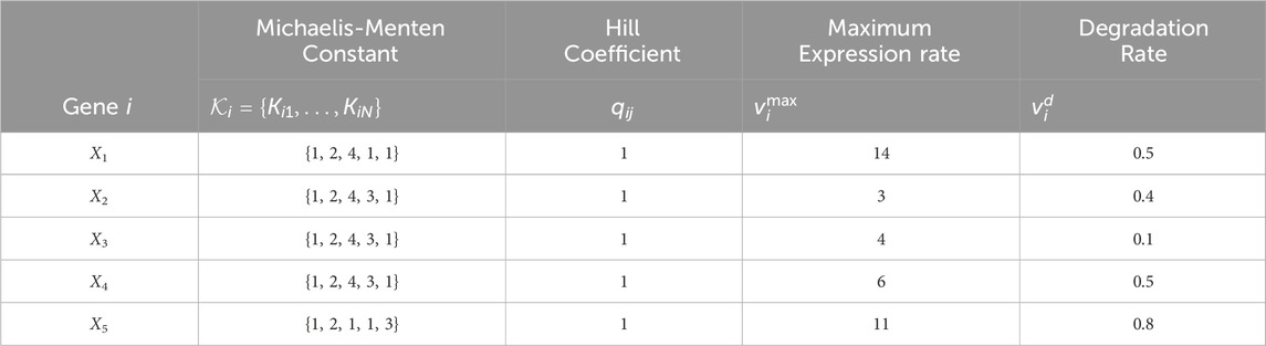
Table 3. Constant parameter values for the GRN models with N = 5 genes in Figure 2. The parameter values correspond to those in the nonlinear dynamic GRN equation in Eq. 4.

Table 4

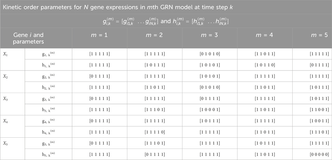
Table 4. Time-varying kinetic order parameters for M = 5 GRN models with N = 5 genes in Figure 2. Each m denotes a specific GRN configuration which is parameterized by g and h. These parameters correspond to those in Eq. 7.

The BLT implementation using the PF and Gibbs sampling follows Algorithm 1. In the simulations, the modeling error process and measurement noise process are both assumed Gaussian with zero-mean and uncorrelated samples; their corresponding unknown covariance matrices are ${\mathrm{\Sigma }}_{\mathbf{w}}^{(m)}={\text{var}}_{\mathbf{w},m}{I}_N$ and Σ_v = var_vI_N. Here, var_w,m and var_v denote their respective variance values and I_N is the N × N identity matrix. At each time step k, k = 1, …, K, our learning approach concurrently estimates the unknown expression levels and the configuration model. We use the categorical distribution over M values whose vector parameter is learned using the Dirichlet distribution conjugate prior with hyperparameter α; in the simulations, we use α_m = 1, m = 1, …, M. We place IWD conjugate priors over the unknown covariance matrices with initial hyperparamers {Ψ₀, ν₀} = {0.1I_N, N + 2}. We demonstrate the robustness of our approach across different sequences of gene regulation configurations. Unless otherwise specified, the simulations use 1,000 particles, 50,000 Monte Carlo runs and 10,000 Gibbs iterations.

3.2 Simulation results

We consider three different simulation scenarios with a varying number of configuration models during different time step segments, as summarized in Table 5. In the table, ${\mathcal{T}}_{l,m}$ denotes the lth time segment during which the mth model is used. The description of each model is provided in Section 3.1. We selected similar modeling error and measurement noise variances as in (Noor et al., 2012). We compare the performance of our proposed BLT approach with the PF that performs tracking without any learning. The PF assumes that the GRN dynamics are only described by one of the M models in each scenario and uses 0.00003 for both the modeling error and measurement noise variances. These low variance values ensure improved estimation performance for the PF if the model is known, even though the actual variances are not learned.

Table 5

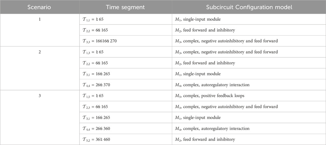
Table 5. GRN configuration models as they vary with time in the simulation scenarios. Time segment ${\mathcal{T}}_{l,m}$ denotes the lth time step duration during which the mth model is used.

Scenario 1: Three-model transition.

The BLT considers an unknown number of TV transitions between M = 3 models: M₁ in Figure 2A during ${\mathcal{T}}_{\mathrm{1,1}}=1:65$, M₂ in Figure 2B during ${\mathcal{T}}_{\mathrm{2,2}}=66:165$, and M₃ in Figure 2C during ${\mathcal{T}}_{\mathrm{3,3}}=66:165$. The PF assumes the M₁ GRN configuration over all time steps. We simulate five different measurement noise variance values, var_v = {2, 0.2, 0.03, 0.003, 0.00003}, and we use var_w,1 = 0.00002, var_w,2 = 0.0005 and var_w,3 = 0.00004 for the actual values of the modeling error variances. The resulting root mean-square error (RMSE), averaged over all time steps, for estimating the gene expression levels using the BLT is provided in Table 6. The averaged RMSE for varying process noise intensities is shown in Table 7. As expected, the RMSE decreases as var_v increases. Using var_v = 0.003, Figure 3 and Figure 4 further demonstrate the performance of the proposed BLT approach. Figure 3 compares the true expression levels of each of the 5 genes to those estimated by the BLT and PF methods. As demonstrated, the PF performed well during the first time segment as it assumed the correct model M₁. However, the estimation performance deteriorated when the network architecture changed. In contrast, the BLT accurately estimated the gene expressions by learning the model transition probabilities and unknown noise variances. Figure 4 compares the actual model labels with those learned by the BLT. Note that after only two initial incorrect estimates, the BLT learned the correct model at each change in model transition. For the same modeling error variances, Figure 5 compares the true and estimated model labels when the measurement noise variance is var_v = 0.2. As it can be seen, as the noise in the measurements increases, the number of incorrect labels also increases. In Figure 6, we increased the modeling error variances to var_w,1 = 0.002, var_w,2 = 0.004 and var_w,3 = 0.005 and kept the measurement noise variance to var_v = 0.003. We observed that the model estimation accuracy is more sensitive to increased modeling error variances. Note that changing the time segments of the different models produced similar RMSE results, thus demonstrating the robustness of our Bayesian learning algorithm for the three-model case.

Table 6

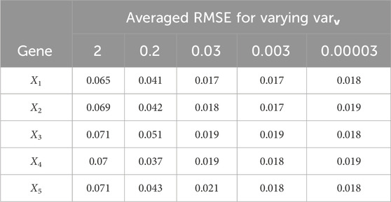
Table 6. Scenario 1: Averaged gene expression estimation RMSE for varying measurement noise variance var_v; the modeling error variances were var_w,1 = 0.00002, var_w,2 = 0.0005, var_w,3 = 0.00004.

Table 7

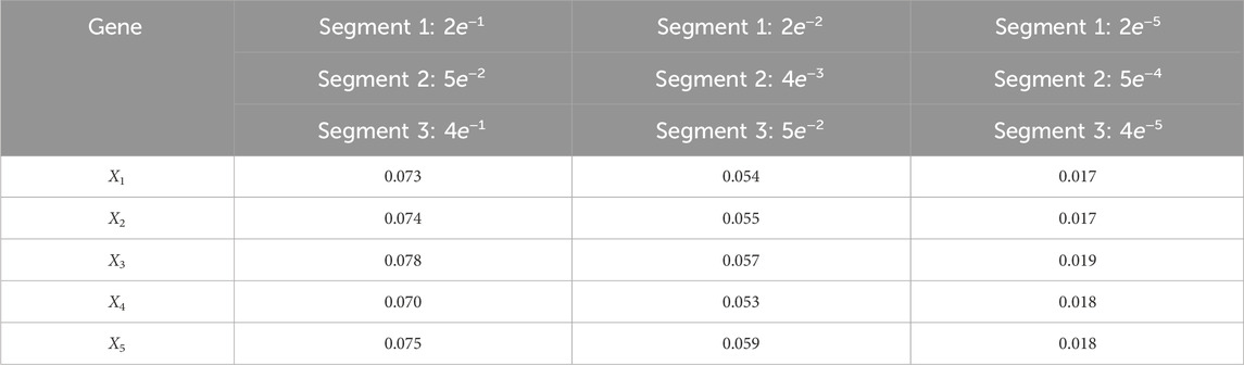
Table 7. Averaged RMSE for varying process noise intensities. For time steps k = 1: 65, the dynamics are described by model 1; for time steps k = 66: 165, the dynamics are described by model 2; and for time steps k = 166: 270, the dynamics are described by model 3. We use 1,000 particles, 5,000 Monte Carlo runs and 10,000 Gibbs iterations were used.

Figure 3

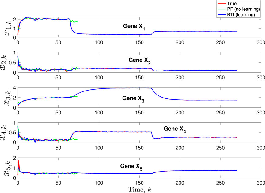
Figure 3. Scenario 1: Comparison of true, PF estimated and BLT estimated expression level x_i,k of Gene X_i, i = 1, …, 5 using modeling error variances var_w,1 = 0.00002, var_w,2 = 0.0005, var_w,3 = 0.00004 and measurement noise variance var_v = 0.003.

Figure 4

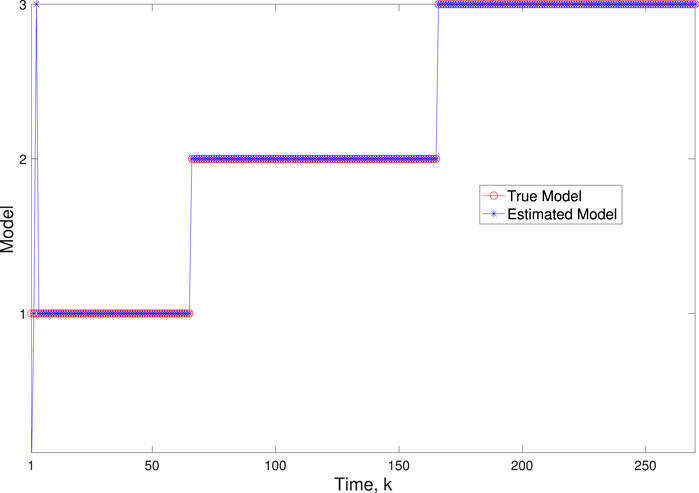
Figure 4. Scenario 1: Comparison of true and BLT estimated labels using var_w,1 = 0.00002, var_w,2 = 0.0005, var_w,3 = 0.00004, and var_v = 0.003.

Figure 5

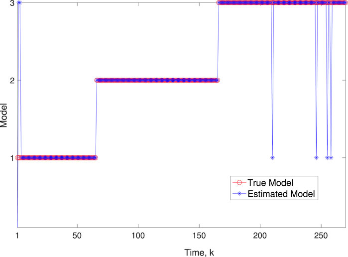
Figure 5. Scenario 1: Comparison of true and BLT estimated labels using var_w,1 = 0.00002, var_w,2 = 0.0005, var_w,3 = 0.00004 and var_v = 0.2.

Figure 6

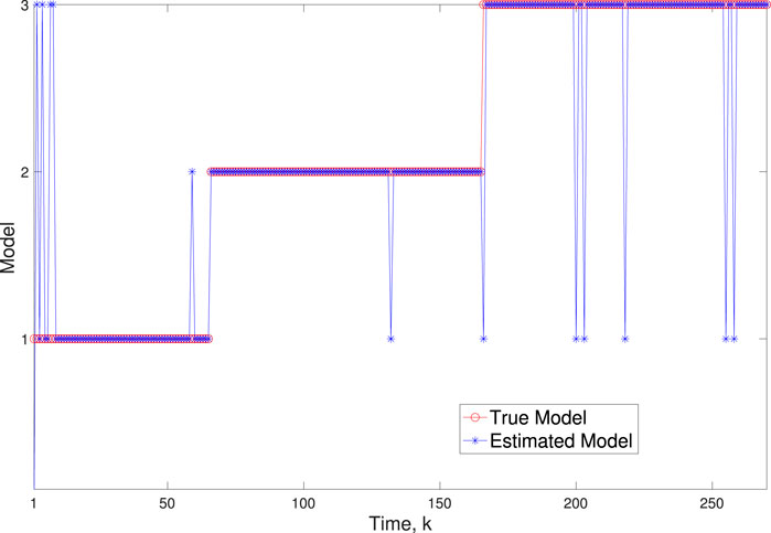
Figure 6. Scenario 1: Comparison of true and BLT estimated labels using var_w,1 = 0.02, var_w,2 = 0.004, var_w,3 = 0.005 and var_v = 0.003.

Scenario 2: Four-model transition.

In this scenario, the BLT considers transitions between M = 4 models: M₃ in Figure 2C during ${\mathcal{T}}_{\mathrm{1,3}}=1:65$, M₂ in Figure 2B during ${\mathcal{T}}_{\mathrm{2,2}}=66:165$, M₁ in Figure 2C during ${\mathcal{T}}_{\mathrm{3,1}}=166:265$, and M₄ in Figure 2D during ${\mathcal{T}}_{\mathrm{4,4}}=266:370$. The PF assumes that model M₃ is used for all time steps. We simulate five different measurement noise variance values, var_v = {2, 0.2, 0.03, 0.003, 0.00003}, and we use var_w,1 = 0.00002, var_w,2 = 0.0005, var_w,3 = 0.00004 and var_w,4 = 0.0002 for the actual values of the modeling error variances. The gene expression averaged RMSE using the BLT are provided in Table 8 and Table 9. As expected, the RMSE increases as var_v increases.

Table 8

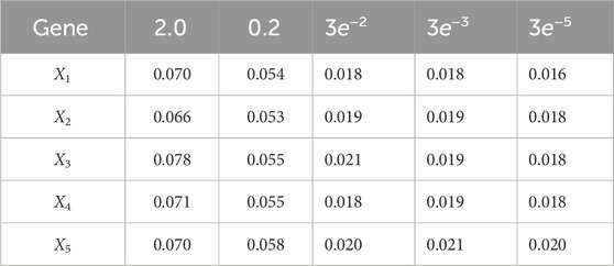
Table 8. Root mean-square error (RMSE) averaged across all time steps for varying measurement noise intensities. For time steps k = 1: 65, the dynamics are described by model 3; for time steps k = 66: 165, the dynamics are described by model 2; for time steps k = 166: 265, the dynamics are described by model 1; and for k = 265: 370, the dynamics are described by model 4. We use 1,000 particles, 5,000 Monte Carlo runs and 10,000 Gibbs iterations were used.

Table 9

Table 9. Root mean-square error (RMSE) averaged across all time steps for varying process noise intensities. For time steps k = 1: 65, the dynamics are described by model 3; for time steps k = 66: 165, the dynamics are described by model 2; for time steps k = 166: 265, the dynamics are described by model 1; and for k = 265: 370, the dynamics are described by model 4. We use 1,000 particles, 5,000 Monte Carlo runs and 10,000 Gibbs iterations were used.

A comparison of our learning algorithm to the standard PF (no learning) is shown in Figure 7 for var_v = 0.003. The standard PF (no learning method) assumes that the dynamics are only described by M₃. As in scenario 1, the standard particle filter (no learning) can only provide estimates of the gene expressions whose trajectories are described by M₃. Until the network architecture switches. Then it is no longer able to estimate the trajectory. In contrast, the BLT is able to estimate the trajectory at each of the change points. The true versus estimated model for different noise values are shown in Figure 8, Figure 9, Figure 10, which demonstrates that the BLT effectively estimates the correct model. The RMSE across different measurement noise intensity values is shown in Table 8. We also vary the modeling error variance and the RMSE values are shown in Table 9. Figure 9 further demonstrates the performance of the proposed BLT approach under high measurement noise conditions. Figure 10 demonstrates the BLT performance under increased modeling error variance.

Figure 7

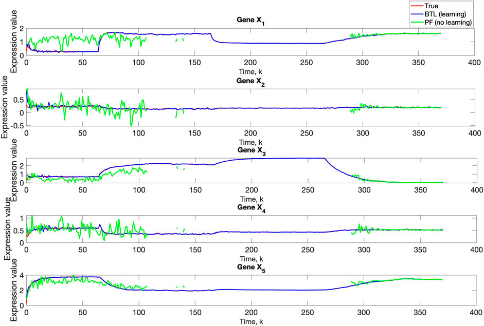
Figure 7. Comparison of true, PF estimated and BLT estimated expression level x_i,k of Gene X_i, i = 1, …, 5 in Scenario 2. The TV model configuration is provided in Table 5.

Figure 8

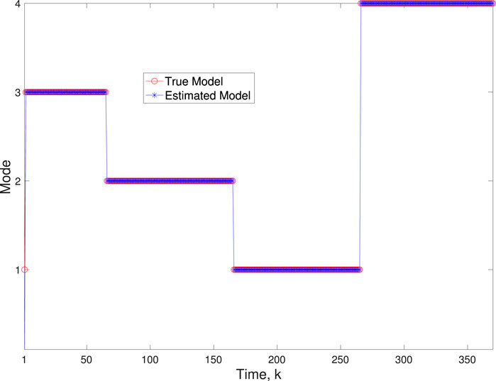
Figure 8. Scenario 2: Comparison of true and BLT estimated labels using var_w,1 = 0.00002, var_w,2 = 0.0005, var_w,3 = 0.00004, var_w,3 = 0.0002, and var_v = 0.003.

Figure 9

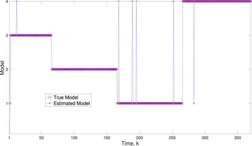
Figure 9. Scenario 2: Comparison of true and BLT estimated labels using var_w,1 = 0.00002, var_w,2 = 0.0005, var_w,3 = 0.00004, var_w,3 = 0.0002, var_v = 2.

Figure 10

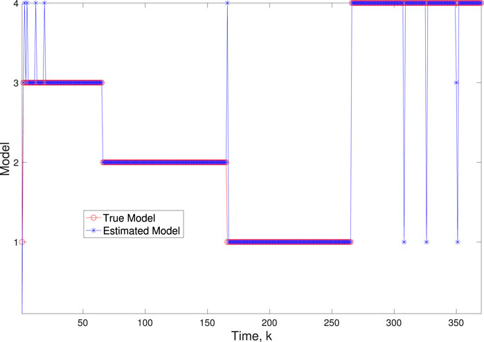
Figure 10. Scenario 2: Comparison of true and BLT estimated labels using var_w,1 = 0.02, var_w,2 = 0.004, var_w,3 = 0.05, var_w,3 = 0.002, var_v = 0.003.

Scenario 3: Transitions Among Five Models.

In this scenario, the BLT considers transitions between M = 5 models: M₃ in Figure 2C during ${\mathcal{T}}_{\mathrm{1,5}}=1:65$, M₂ in Figure 2B during ${\mathcal{T}}_{\mathrm{2,3}}=66:165$, M₁ in Figure 2C during ${\mathcal{T}}_{\mathrm{3,1}}=166:265$, M₄ in Figure 2D during ${\mathcal{T}}_{\mathrm{4,4}}=266:360$. And M₅ in Figure 2E during ${\mathcal{T}}_{\mathrm{5,2}}=361:460$. The time series consists of K = 460 time steps. We simulate five different measurement noise variance values, var_v = {2, 0.2, 0.03, 0.003, 0.00003}, For each simulation where the measurement noise is varied, the true values of var_w,1 = 0.00002, var_w,2 = 0.0005, var_w,3 = 0.00004, var_w,4 = 0.0002, var_w,5 = 0.003.

Using var_v = 0.02, Figure 11 and Figure 12 further demonstrate the performance of the proposed BLT approach. Figure 11 compares the true expression levels of each of the 5 genes to those estimated by the BLT and PF methods. As in the previous scenarios, the standard particle filter (no learning) is only able to estimate the trajectory during the third segment where model M₁ is assumed. Then it is no longer able to estimate the trajectory. In contrast, the BLT method is able to estimate the trajectory at each of the change points. Figure 12 compares the actual model labels with those learned by the BLT. The averaged RMSE for varying measurement and process noise intensities are shown in Tables 10 and 11, respectively. Note that the BLT algorithm exhibits similar performance to the previous scenarios despite increasing the number of models to M = 5.

Figure 11

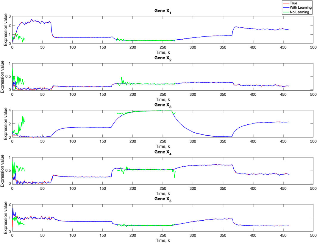
Figure 11. Comparison of true, PF estimated and BLT estimated expression level x_i,k of Gene X_i, i = 1, …, 5 in Scenario 3. The TV model configuration is provided in Table 5.

Figure 12

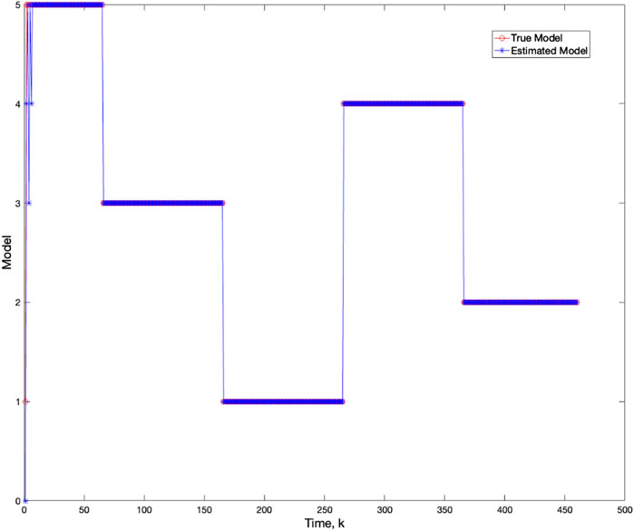
Figure 12. Comparison of true and BLT estimated labels of the configuration models in Scenario 3.

Table 10

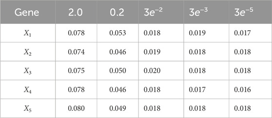
Table 10. Root mean-square error (RMSE) averaged across all time steps for varying measurement noise intensities. For time steps k = 1: 65, the dynamics are described by model 5; for time steps k = 66: 165, the dynamics are described by model 3; for time steps k = 166: 265, the dynamics are described by model 1; for k = 265: 360, the dynamics are described by model 4; and for k = 360: 460 the dynamics are described by model 5. We use 1,000 particles, 5,000 Monte Carlo runs and 10,000 Gibbs iterations were used.

Table 11

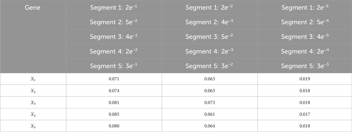
Table 11. Root mean-square error (RMSE) averaged across all time steps for varying process noise intensities. For time steps k = 1: 65, the dynamics are described by model 5; for time steps k = 66: 165, the dynamics are described by model 3; for time steps k = 166: 265, the dynamics are described by model 1; for k = 265: 370, the dynamics are described by model 4; and for k = 371: 460, the dynamics are described by model 2. We use 1,000 particles, 5,000 Monte Carlo runs and 10,000 Gibbs iterations were used.

4 Conclusion and future directions

In this work, we introduced a fully Bayesian hierarchical model for learning nonlinear gene regulatory networks with dynamically switching subcircuit architectures. We showed that our algorithm, which employs sequential Monte Carlo (SMC) with a local Gibbs step, effectively estimates the correct model corresponding to the subcircuit architecture as well as the unknown state under varying measurement and process noise conditions with a high degree of accuracy, though with greater sensitivity to variations in the process noise. Through the use of conjugate priors, we have formulated an analytically tractable inference scheme which effectively addresses the challenges posed by the inherent complexities of the system. By learning the unknown transition probabilities, which describe changes between different network configurations and by learning the unknown measurement and process noise covariances using Bayesian updating of the Inverse-Wishart distribution, we were able to account for uncertainty at all levels of the hierarchy. Our approach has demonstrated robustness and versatility in identifying changes in subcircuit architectures of varying degrees of complexity, ranging from a simple single-input-module (SIM) to subcircuits consisting of a composition of different types. To showcase this robustness, we applied our algorithm to different scenarios where the architecture switches between three, four, and five types.

It is worth noting that the methodology developed in this work is not confined to the analysis of gene regulatory networks but can also be generalized to other domains which involve switching dynamics in nonlinear systems. For example, our methodology can be applied to change point detection problems in financial markets, where a sudden shift in the market dynamics could be caused by changes in nonlinear interactions between different economic factors. While our Bayesian hierarchical model offers an effective and robust framework for learning switching dynamics in nonlinear gene regulatory networks, the complexity of the SMC algorithm with a local Gibbs step poses computational challenges. The drawbacks of incorporating Gibbs within SMC include potential inefficiencies, particularly in large-scale systems, where the iterative Gibbs sampling step at each stage of the sequential updating process may lead to increased computational burden. This challenge is accentuated when dealing with multi-omics data. As such, future research aims to extend our methodology to large-scale systems through the use of stochastic gradient Markov Chain Monte Carlo (SGMCMC), leveraging its efficiency in handling high-dimensional data and providing a computationally scalable approach for the analysis of switching gene regulatory networks.

Data availability statement

The original contributions presented in the study are included in the article/Supplementary Material, further inquiries can be directed to the corresponding author/s.

Author contributions

NV-C: Conceptualization, Formal Analysis, Investigation, Methodology, Writing–original draft, Writing–review and editing. AP-S: Conceptualization, Supervision, Writing–original draft, Writing–review and editing.

Funding

The author(s) declare that financial support was received for the research, authorship, and/or publication of this article. This work was partially funded by AFOSR grant FA9550-23-1-0328.

Conflict of interest

The authors declare that the research was conducted in the absence of any commercial or financial relationships that could be construed as a potential conflict of interest.

Publisher’s note

All claims expressed in this article are solely those of the authors and do not necessarily represent those of their affiliated organizations, or those of the publisher, the editors and the reviewers. Any product that may be evaluated in this article, or claim that may be made by its manufacturer, is not guaranteed or endorsed by the publisher.

Supplementary material

The Supplementary Material for this article can be found online at: https://www.frontiersin.org/articles/10.3389/frsip.2024.1323538/full#supplementary-material

References

Alon, U. (2019) An introduction to systems biology: design principles of biological circuits. United States: CRC Press.

Google Scholar

Amor, N., Meddeb, A., Marrouchi, S., and Chebbi, S. (2019). A comparative study of nonlinear bayesian filtering algorithms for estimation of gene expression time series data. Turkish J. Electr. Eng. Comput. Sci. 27, 2648–2665. doi:10.3906/elk-1809-187

CrossRef Full Text | Google Scholar

Ancherbak, S., Kuruoglu, E. E., and Vingron, M. (2016). Time-dependent gene network modelling by sequential Monte Carlo. IEEE/ACM Trans. Comput. Biol. Bioinforma. 13, 1183–1193. doi:10.1109/TCBB.2015.2496301

PubMed Abstract | CrossRef Full Text | Google Scholar

Arulampalam, M. S., Maskell, S., Gordon, N., and Clapp, T. (2002). A tutorial on particle filters for online nonlinear/non-Gaussian Bayesian tracking. IEEE Trans. Signal Process. 50, 174–188. doi:10.1109/78.978374

CrossRef Full Text | Google Scholar

Bugallo, M. F., Taşdemir, c., and Djurić, P. M. (2015). “Estimation of gene expression by a bank of particle filters,” in 2015 23rd European Signal Processing Conference (EUSIPCO), Nice, France, 31 August - 4 September 2015, 494–498.

CrossRef Full Text | Google Scholar

Chopin, N. (2002). A sequential particle filter method for static models. Biometrika 89, 539–552. doi:10.1093/biomet/89.3.539

CrossRef Full Text | Google Scholar

Dondelinger, F., Lebre, S., and Husmeier, D. (2013). Non-homogeneous dynamic bayesian networks with bayesian regularization for inferring gene regulatory networks with gradually time-varying structure. Mach. Learn. 90, 191–230. doi:10.1007/s10994-012-5311-x

CrossRef Full Text | Google Scholar

Elahi, F., and Hasan, A. (2018). A method for estimating hill function-based dynamic models of gene regulatory networks. R. Soc. Open Sci. 5, 171226. doi:10.1098/rsos.171226

PubMed Abstract | CrossRef Full Text | Google Scholar

Elvira, V., Martino, L., Bugallo, M. F., and Djuric, P. M. (2019). Elucidating the auxiliary particle filter via multiple importance sampling [lecture notes]. IEEE Signal Process. Mag. 36, 145–152. doi:10.1109/MSP.2019.2938026

CrossRef Full Text | Google Scholar

Gelfand, A. E., Hills, S. E., Racine-Poon, A., and Smith, A. F. M. (1990). Illustration of Bayesian inference in normal data models using Gibbs sampling. J. Am. Stat. Assoc. 85, 972–985. doi:10.1080/01621459.1990.10474968

CrossRef Full Text | Google Scholar

Gelman, A., Carlin, J. B., Stern, H. S., and Rubin, D. B. (1995) Bayesian data analysis. United States: Chapman and Hall/CRC.

Google Scholar

Ha, D., Kim, D., Kim, I., Oh, Y., Kong, J., Han, S., et al. (2022). Evolutionary rewiring of regulatory networks contributes to phenotypic differences between human and mouse orthologous genes. Nucleic Acids Res. 50, 1849–1863. doi:10.1093/nar/gkac050

PubMed Abstract | CrossRef Full Text | Google Scholar

Hinman, V. F., and Cheatle Jarvela, A. M. (2014). Developmental gene regulatory network evolution: insights from comparative studies in echinoderms. genesis 52, 193–207. doi:10.1002/dvg.22757

PubMed Abstract | CrossRef Full Text | Google Scholar

Krishnan, M., Small, M., Bosco, A., and Stemler, T. (2020). Network using Michaelis-Menten kinetics: constructing an algorithm to find target genes from expression data. J. Complex Netw. 8. doi:10.1093/comnet/cnz016

CrossRef Full Text | Google Scholar

Lee, D. S., and Chia, N. K. (2002). A particle algorithm for sequential Bayesian parameter estimation and model selection. IEEE Transaction Signal Process. 50, 326–336. doi:10.1109/78.978387

CrossRef Full Text | Google Scholar

Lee, T. H., Lakshmanan, S., Park, J. H., and Balasubramaniam, P. (2013). State estimation for genetic regulatory networks with mode-dependent leakage delays, time-varying delays, and markovian jumping parameters. IEEE Trans. NanoBioscience 12, 363–375. doi:10.1109/TNB.2013.2294478

PubMed Abstract | CrossRef Full Text | Google Scholar

Li, Y., Papandreou-Suppappola, A., and Morrell, D. (2006). “Instantaneous frequency estimation using sequential Bayesian techniques,” in Asilomar Conference on Signals, Systems, and Computers, Oct. 27th - Oct. 30th, 2024, 569–573.

CrossRef Full Text | Google Scholar

Martino, L., Elvira, V., and Camps-Valls, G. (2018). The recycling gibbs sampler for efficient learning. Digit. Signal Process. 74, 1–13. doi:10.1016/j.dsp.2017.11.012

CrossRef Full Text | Google Scholar

McKenzie, G. J., Harris, R. S., Lee, P. L., and Rosenberg, S. M. (2000). The sos response regulates adaptive mutation. Proc. Natl. Acad. Sci. U. S. A. 97, 6646–6651. doi:10.1073/pnas.120161797

PubMed Abstract | CrossRef Full Text | Google Scholar

Mittal, N., Guimaraes, J., Gross, T., Schmidt, A., Vina, A., Nedialkova, D., et al. (2017). The gcn4 transcription factor reduces protein synthesis capacity and extends yeast lifespan. Nat. Commun. 8, 457. doi:10.1038/s41467-017-00539-y

PubMed Abstract | CrossRef Full Text | Google Scholar

Nadal, E., and Posas, F. (2022). The hog pathway and the regulation of osmoadaptive responses in yeast. FEMS Yeast Res. 22, foac013. doi:10.1093/femsyr/foac013

PubMed Abstract | CrossRef Full Text | Google Scholar

Noor, A., Serpedin, E., Nounou, M., and Nounou, H. (2012). Inferring gene regulatory networks via nonlinear state-space models and exploiting sparsity. IEEE/ACM Trans. Comput. Biol. Bioinforma. 9, 1203–1211. doi:10.1109/TCBB.2012.32

PubMed Abstract | CrossRef Full Text | Google Scholar

Peter, I. S., and Davidson, E. H. (2011). Evolution of gene regulatory networks controlling body plan development. Cell 144, 970–985. doi:10.1016/j.cell.2011.02.017

PubMed Abstract | CrossRef Full Text | Google Scholar

Peter, I. S., and Davidson, E. H. (2015) Genomic control process: development and evolution. Massachusetts, United States: Academic Press.

Google Scholar

Pirgazi, J., and Khanteymoori, A. R. (2018). A robust gene regulatory network inference method base on kalman filter and linear regression. PLOS ONE 13, 02000944–e200117. doi:10.1371/journal.pone.0200094

PubMed Abstract | CrossRef Full Text | Google Scholar

Potkin, S. G., Macciardi, F., Guffanti, G., Fallon, J. H., Wang, Q., Turner, J. A., et al. (2010). Identifying gene regulatory networks in schizophrenia. NeuroImage 53, 839–847. doi:10.1016/j.neuroimage.2010.06.036

PubMed Abstract | CrossRef Full Text | Google Scholar

Saunders, L., and McClay, D. (2014). Sub-circuits of a gene regulatory network control a developmental epithelial-mesenchymal transition. Dev. Camb. Engl. 141, 1503–1513. doi:10.1242/dev.101436

PubMed Abstract | CrossRef Full Text | Google Scholar

Sudderth, E. (2016). Conjugate priors and Bayesian learning. Lect. Notes.

Google Scholar

Tsigos, C., and Chrousos, G. P. (2002). Hypothalamic–pituitary–adrenal axis, neuroendocrine factors and stress. J. Psychosomatic Res. 53, 865–871. doi:10.1016/S0022-3999(02)00429-4

PubMed Abstract | CrossRef Full Text | Google Scholar

Vélez-Cruz, N., Moraffah, B., and Papandreou-Suppappola, A. (2021). “Sequential Bayesian inference using stochastic models of gene regulatory networks,” in Asilomar Conference on Signals, Systems, and Computers, Oct. 27th - Oct. 30th, 2024, 568–572.

Google Scholar

Wang, H., Qian, L., and Dougherty, E. (2007). “Inference of gene regulatory networks using s-system: a unified approach,” in 2007 IEEE Symposium on Computational Intelligence and Bioinformatics and Computational Biology, Hawaii, USA, April 1-5, 2007, 82–89.

Google Scholar

Wang, Z., Liu, X., Liu, Y., Liang, J., and Vinciotti, V. (2009). An extended kalman filtering approach to modeling nonlinear dynamic gene regulatory networks via short gene expression time series. IEEE/ACM Trans. Comput. Biol. Bioinforma. 6, 410–419. doi:10.1109/TCBB.2009.5

PubMed Abstract | CrossRef Full Text | Google Scholar

Xiong, J., and Zhou, T. (2013). A kalman-filter based approach to identification of time-varying gene regulatory networks. PLOS ONE 8, e74571–e74578. doi:10.1371/journal.pone.0074571

PubMed Abstract | CrossRef Full Text | Google Scholar

Youseph, A. S. K., Chetty, M., and Karmakar, G. (2015). “Gene regulatory network inference using michaelis-menten kinetics,” in 2015 IEEE Congress on Evolutionary Computation (CEC), Sendai, Japan, 25-28 May 2015, 2392–2397.

CrossRef Full Text | Google Scholar

Youseph, A. S. K., Chetty, M., and Karmakar, G. (2019). Reverse engineering genetic networks using nonlinear saturation kinetics. Biosystems 182, 30–41. doi:10.1016/j.biosystems.2019.103977

PubMed Abstract | CrossRef Full Text | Google Scholar

Zhang, Y., Pu, Y., Zhang, H., Cong, Y., and Zhou, J. (2014). An extended fractional kalman filter for inferring gene regulatory networks using time-series data. Chemom. Intelligent Laboratory Syst. 138, 57–63. doi:10.1016/j.chemolab.2014.07.007

CrossRef Full Text | Google Scholar