 Taeer Weiss1
 Tirza Routtenberg
 Jonatan Ostrometzky
 Hagit Messer
- 1School of Electrical Engineering, Tel Aviv University, Tel Aviv, Israel
- 2Department of Electrical and Computer Engineering, Faculty of Engineering Sciences, Ben-Gurion University of the Negev, Beer-Sheva, Israel
This work focuses on optimizing the estimation of accumulated rain from measurements of the attenuation level of signals from commercial microwave links (CMLs). The process of accumulated rain estimation is usually based on estimation after detection, where it is first determined whether there is rain for a specific period, and then the accumulated rain at the detected rainy period is estimated. Naturally, errors in detection affect the accuracy of the consequent accumulated rain estimation. Traditionally, the detection and the estimation steps are designed independently. The detection threshold is arbitrarily set at the lowest level that would be declared as rain, without considering its effect on the accuracy of the accumulated rain estimation. This study applies a novel method that sets a detection threshold to optimize estimation after detection and apply it for accumulated rain estimation. It is based on optimizing a post-detection estimation risk function that incorporates both the estimation and detection-related errors; this essentially takes into consideration the coupling of the detection and the estimation stages and thus optimizes the overall accumulated rainfall estimation. The proposed approach is applied to actual CML attenuation measurements taken from a cellular network in Gothenburg, Sweden. This demonstrates that the proposed method achieves better accuracy for accumulated rain estimation compared with the detection threshold being set independently.
1 Introduction
The task of rain estimation based on attenuation measurements from commercial microwave links (CMLs) has attracted much focus after first being introduced by Messer et al. (2006) and developed in studies such as Ostrometzky and Messer (2014), D’Amico et al. (2016), Ostrometzky et al. (2015), Graf et al. (2020), Overeem et al. (2013), and Fencl et al. (2015).
CMLs as opportunistic sensors for rain monitoring can be used either as an additional layer of meteorological sensors (mainly in developed countries) or as stand-alone rain-monitoring infrastructure (mainly in the developing world) where other meteorological instrumentation is sparse (Zhang et al., 2023). In general, CML hardware is controlled by a network management system or can be accessed by network providers directly to log and report the transmitted signal level (TSL) and received signal level (RSL) time series using sampling intervals of seconds to minutes (Messer and Sendik, 2015). The channel attenuation can thus be directly calculated.
The accuracy of the accumulated rain estimation is highly affected by the preliminary detection step, in which it is detected whether a specific time frame is wet or dry. Errors in the preliminary detection step create bias in the subsequent estimation step. In particular, misdetecting rain events will result in the underestimation of the accumulated rain. Similarly, falsely detecting a dry or “no rain” event as rainy will result in overestimation of the accumulated rain. Therefore, careful design of the detection step can optimize the performance of both detection and estimation and reduce inherent bias.
Distinguishing between attenuation due to rain and other-than-rain attenuation is challenging since the attenuation baseline fluctuates due to variations in water vapor concentration, temperature, wind effects, and other phenomena (both during a rain event and dry periods). Nonetheless, since rain is the major factor of attenuation for CMLs operating at the K- and E-band frequency ranges (ITU-R.530, 2009; ITU-R.838, 2005) and its presence introduces attenuation components other than Gaussian measurement noise, it is challenging to detect and estimate rain using CML attenuation measurements. Extraction of the rain-induced components from the attenuation signal is achieved using different methods—see reviews in Zhang et al. (2023) and Chwala and Kunstmann (2019). However, these approaches are based on pre-set thresholds for detecting rainy periods, followed by rain estimation.
In order to obtain meaningful rain-intensity estimations from CMLs, most current approaches focusing on the preliminary task of classifying between wet and dry periods rely on a test with comparisons based on a pre-set threshold. For instance, in Rahimi et al. (2003), wet and dry events were distinguished by a test based on the correlation between the RSL for different frequencies, as the rain affects each frequency differently. In Goldshtein et al. (2009), the classification test used the time-domain correlation of bidirectional CML signals. In Overeem et al. (2016), wet periods are identified by analyzing the temporal correlation of different CMLs in the same area, as it is assumed that, when rain is present, its effects on nearby CMLs will be similar, and, thus, the correlation between the CML attenuation signals will increase (compared to dry periods, in which additive noise plays a more significant role on the attenuation variations). Schleiss and Berne (2010) adopt another approach by presenting a wet/dry classification test by analyzing the local variability of the CML signal. Such local variability of the CML signals during rainy events can also be detected in the frequency domain, as demonstrated by another wet/dry classification method, by analyzing the spectra of the signal fluctuations (Chwala et al., 2012). In Wang et al. (2012), wet/dry classification was performed based on Markov switching models. These approaches (among many others) leveraged the fact that, during rain events, attenuation signals properties (such as variance, correlation with different nearby CMLs, or absolute values) change in a meaningful and detectable manner. Moreover, when historical data for training are available, machine learning approaches designed to classify between wet and dry periods have demonstrated good results (e.g., Habi and Messer (2018) and Polz et al. (2020)). Precipitation classification using a decision tree method was performed by Cherkassky et al. (2013). However, in all the above, the setting of a detection threshold is arbitrary—there is no methodology for setting it to detect a rainy period with respect to false alarms and the misdetect ratio, which could potentially optimize the consequent estimation approach.
The contribution in this work is in applying an advanced statistical signal processing tool to accumulated rainfall monitoring from wireless communication measurements. We show that a detection threshold that optimizes a novel risk function, proposed in Weiss et al. (2021), can be applied to a real-world application of estimation after detection, and that implementing that threshold in this application improves the accuracy of accumulated rainfall estimation. We therefore propose a new method for estimating total accumulated rain by taking into consideration the preliminary detection step. In particular, we analyze the effects of the coupling of each step’s error for the first time in this particular application. The detection stage is performed by comparing a function of the signal attenuation measurements against a threshold. The threshold is set by optimizing a risk function that incorporates errors that relate to the combined estimation and detection stages (Weiss et al., 2021). Using this risk function, we account for the impact that the detection step might have on the accuracy of the accumulated rain estimation and thus optimize the complete scheme. We tested the proposed approach by applying it to attenuation measurements taken by CMLs of an operational cellular network in Gothenburg, Sweden, and estimated the accumulated rain through periods of 24 h. We show that the detection threshold that optimizes the proposed risk function agrees with the threshold that empirically best matches the estimated accumulated rain, with the value measured by a corresponding rain gauge. In addition, we compare our methodology with a well-established CML-based rain detection approach (Schleiss and Berne, 2010) and show the potential improvement of the overall accuracy of rainfall estimation that our proposed approach offers.
2 Model and performance evaluation measure
2.1 Model
We consider the problem of estimating the accumulated rain from the attenuation level of signals from CMLs, where it should first be decided if there is rain at the tested time frame. This problem can be interpreted as an “intensity estimation after detection” problem (Chaumette et al., 2005; Weiss et al., 2021), where a decision between two hypotheses is first performed (detection) and then, based on the resulting decision, estimation of the unknown parameters under the chosen hypothesis is performed.
The problem of post-detection accumulated rain estimation can be mathematically described as follows. We consider an observation vector, x = [x[0],…,x[N − 1]]T, which includes the attenuation level of signals from CMLs with N samples. Then, we assume a given detector that aims to distinguish between a rain event (hypothesis
where g(⋅) is a function of the data defining the specific detector (detailed in Section 2.3). The accuracy of the detection stage depends on the detection threshold value γ.
We assume that, if there is rain (mathematically, if
where βθ represents the attenuation caused by rain and θ ∈ [0, Θ] is an unknown parameter to be estimated which represents the rain-intensity value (in mm/h). The known range parameter Θ is determined by past experiments in the specific area. The known physical parameter β approximates the conversion from rain intensity to attenuation and depends on environmental conditions, the properties of the CMLs—such as frequency, polarization, rain drop size distribution (DSD), and the surrounding temperature. For the sake of simplicity, the noise sequence ω[0], …, ω[N − 1] is assumed to be Gaussian with zero mean and known variance σ2. In this application, the noise contains components other than the Gaussian measurement noise (Fencl et al., 2020). However, for tractable theoretical analysis, we assume a simplified model, ignoring these components, as well as rain fluctuations during the observation interval.
The accumulated rain estimation after detection method is as follows: given the observation vector of attenuation measurements in time frame x, decide whether these attenuation vector values are induced due to a rain event,
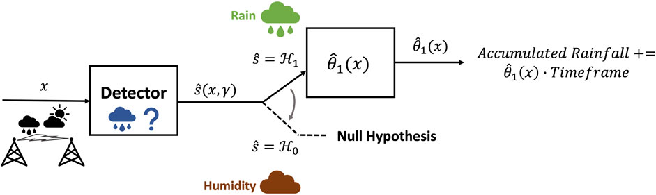
FIGURE 1. Post-rain detection estimation of the accumulated rain: CML-recorded attenuation time series are fed into the detector, which detects whether the attenuation time series is affected by rain. During periods in which rain was detected, an estimation stage was performed in order to establish the accumulated rainfall amount.
2.2 Joint detection–estimation risk
We use a combined performance measure of detection–estimation proposed by Weiss et al. (2021) to set up the system design (i.e., the detection threshold) to improve the accumulated rainfall estimation after detection.
We were specifically interested in the estimation and detection errors associated with the existence of rain, represented by hypothesis
1. Mean squared selected error
Here, the term
2. False alarm risk
Here, the term
3. Misdetection risk
Here, the term
The overall risk is given by
This risk considers both detection and estimation errors, and its minimization aims at optimal estimation after the detection of the accumulated rain. It should be noted that the three terms contributing to the risk (as detailed in (3)–(5)) are all normalized by the maximal rain-intensity value Θ; thus, the obtained risk elements are always between 0 and 1.
This risk function is an adaptation of the risk proposed in Weiss et al. (2021) to the case of a non-Bayesian (frequentist) setting in which only one of the hypotheses is true. This is designed to focus on post-rain-detection estimation, so that errors from “no-rain” periods are irrelevant. Eq. 6 thus compromises three terms: MSSE (which takes into account the probability of the detection of rain in cases where it did occur), the misdetection (MD) term (which takes into account the probability that we decided no rain given that rain occurred), and the false alarm (FA) term (which takes into account the probability that we detected rain but rain was absent).
2.3 Methods
In this subsection, we describe the procedure of post-detection estimation of the accumulated rain from signal attenuation measurements obtained from CMLs over a 24-h period, the calculated risk of (6) for that period, and the proposed detection threshold optimization.
Following the general scheme described in Figure 5.1, the post-detection estimation procedure is implemented as follows: given a vector of signal attenuation measurements over a 24-h period as logged by a CML, we divide the vector into W non-overlapping windows of N samples each. For each window, we decide whether it contains times in which rain fell or not, based on the detector
where
If it detects rain (i.e., chooses hypothesis
The estimated rain intensity is multiplied by the time interval of the window,
During the scan of the W windows of the signal attenuation vector, we calculate 1) mean squared selected error (MSSE) of (3) at times in which rain was correctly detected; 2) RiskFA of (4) at times in which rain was falsely detected during a dry period; 3) RiskMD of (5) at times in which rain was misdetected during a rainy period. These metrics guide the threshold-setting process, prioritizing estimation performance over detection performance.
As ground-truth values for the risk calculation, we use measurements from rain gauges that are located near the CMLs. For rain intensity values, we converted the rain-gauge measurements to mm/h. The classification to “rainy” and “dry” windows’ ground-truth is also based on the rain-gauge measurements. Note that the risk calculation presented is not accurate, especially for windows of long duration, as the calculation is valid under the assumption that the rain intensity remains constant within each window. This is obviously incorrect and will result in an error. However, when considering windows that are relatively short, the resulting error is smaller and thus affects the overall results to only a small degree. The procedures of the post-detection estimation of the accumulated rain and risk calculation were repeated for different threshold values and a different number of windows, W, in the range 100–280 in the first experiment and 23 per day1 in the second experiment.
3 Experimental demonstration
3.1 Data
We demonstrate our presented approach using actual attenuation measurements taken by CMLs. The CMLs operated as part of the backhaul of a cellular network in Gothenburg, Sweden, in 2015–2016. The data were collected by Ericsson AB and the Swedish Meteorological and Hydrological Institute (SMHI). We used four dual-channel CMLs near Gothenburg and their corresponding closest rain gauges. A map of the locations of the four dual-channel CMLs and their corresponding rain gauges is presented in Figure 5.1 in Ostrometzky (2017).
Since being first introduced in Messer et al. (2006), CMLs have been widely used for rain intensity estimation in many scenarios (e.g. Graf et al., 2020; Fencl et al., 2015; Chwala and Kunstmann, 2019; Overeem et al., 2016). Most research has been based on a simplified relationship between rain intensity and rain-induced microwave link attenuation given by the power law (Olsen et al., 1978):
where A is the attenuation due to rain in dB, R is the CML averaged rain rate (in mm/h), L is the microwave link length (in km), and a, b are coefficients determined by the specific CML frequency polarization and by the DSD. Table 5.1 in Ostrometzky (2017) details all relevant properties of the CMLs, which are a subset of the CMLs publicly available in Andersson et al. (2022) and the corresponding power law parameters used in (10) for the four CMLs. For convenience, we summarize the CMLs’ properties in Table 1.

TABLE 1. Properties of the available CMLs: path length (Length), frequency (Freq.), polarization (Pol.), and power law coefficients of (10), taken from ITU.
Based on Tables 1 and (10), we calculated parameter β of (2) by approximating b to be equal to 1 (and thus β = aL).
The data include signal attenuation measurements taken by the four dual-channel CMLs, collected over two 24-h periods: 2 June and 25 July 2015. The attenuation measurement sampling rate was 0.1 Hz (one sample every 10 s), and the measurements are reported in dB. Each CML was coupled with its closest rain gauge. The rain gauges produced measurements at intervals of 1 min, measuring the accumulated rain in the interval (in mm). For more information about the rain gauges and CMLs used, see Ostrometzky (2017).
We evaluate the performance of the proposed approach for the sample-mean detector in Section 3.2 and for the variance detector in Section 3.3.
3.2 First experiment—the sample-mean detector
In the first experiment, we performed the detection using the sample-mean detector from 1 and 7. Figure 2 presents a comparison between 1) the empirical threshold obtained by optimizing the risk and 2) the theoretical threshold that yields the most accurate accumulated rain estimation with respect to (w.r.t.) the ground-truth value from the rain gauges. Each figure presents the results for different dates (2 June or 25 July 2015) and varying window numbers W (100 or 280). In each figure, the first row presents the risk versus the threshold value for the four links, and the second row presents the ground-truth and the accumulated rain estimation versus the threshold. The theoretical threshold is the best threshold according to the accuracy of the accumulated rain estimation w.r.t. the ground truth from the rain gauge is indicated at the intersection of the blue graph and the orange line in the bottom row, showing that there is good resemblance between the theoretical threshold determined in the intersection points and the empirical2 threshold determined by optimizing the risk (the red points) for all values of the number of windows. These results show that the value of the detection threshold that minimizes the proposed risk agrees with the value of the threshold that best matches the estimated accumulated rain with the value measured by the corresponding rain gauge.
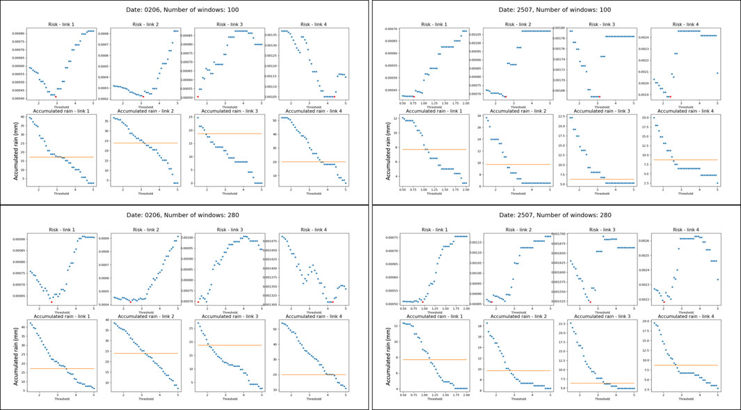
FIGURE 2. Results for W =100 or W =280 for each of the channels a of the CMLs detailed in Table 1. In each panel, the top row presents the risk (in arbitrary units) versus the threshold value (in arbitrary units), where the minimum risk is the point marked in red. The bottom row in each panel presents the accumulated rain estimation (in mm) (blue) and the ground-truth accumulated rain from the rain gauge (orange) versus the threshold.
Figure 3 presents the accumulated rain estimation for the empirical threshold that minimizes the risk versus the ground-truth value of accumulated rain from the rain gauges. Each group of points with the same color represents results from one of the four dual-channel links and on one of the two examined dates. The different points in each group correspond to estimation done with different values of the number of windows W and on different channels. It is apparent that the estimation points fit well with the ground-truth values from the rain gauges, with a slight overestimation. Indeed, the design parameter W, which corresponds to the number of windows, affects the accuracy of a given scenario. Figure 4 presents the empirical threshold that minimizes the risk (corresponding to the red points in Figure 2) versus the theoretical threshold that yields the most accurate estimation w.r.t. the rain gauge (corresponding to the intersection points of the blue and orange graphs in Figure 2). Like Figure 3, each group of points represents estimation from a single link at a specific date, and the different points correspond to a different number of windows and channels. It is apparent that the empirical threshold values fit the theoretical ones well, with a slight underestimation of the threshold which results in an overestimation of the accumulated rain (Figure 3).
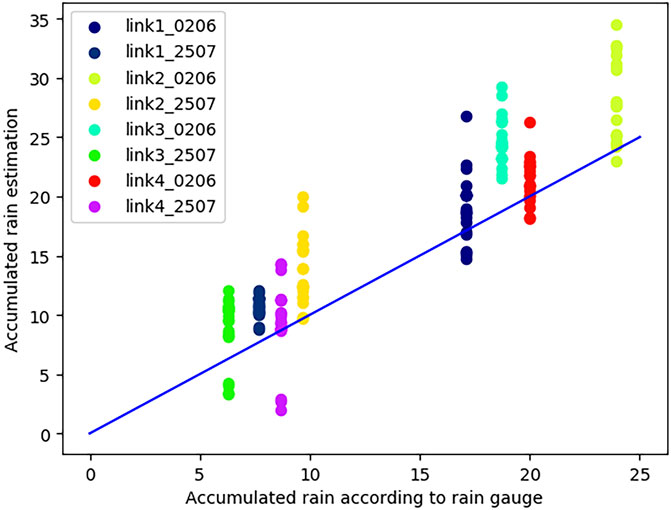
FIGURE 3. Accumulated rain estimation from the CMLs (channel a from Table 1) versus accumulated rain according to the rain gauge. Each group of points with the same color represents estimation based on one dual-channel link for different dates and varying window numbers, W.
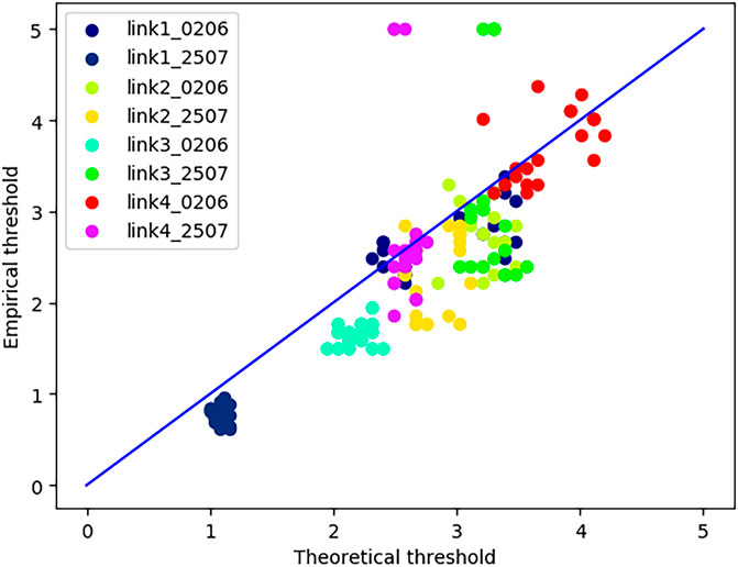
FIGURE 4. Empirical versus theoretical threshold. Each group of points with the same color represents estimation based on one dual-channel link for different dates and varying window numbers, W.
As can be seen in Figure 2, different thresholds minimize the risk for a specific link on different days. This raises the question of how to select one threshold that will be used for a specific link. For that purpose, we tested the accumulated rainfall estimation performance when one threshold is applied in each direction of the link for all dates. The threshold we took is the average of the threshold values that minimize the risk on the different dates. The results are presented in Figure 5, which shows that, in most cases and rain events, taking the same averaged threshold value per link produces good results.
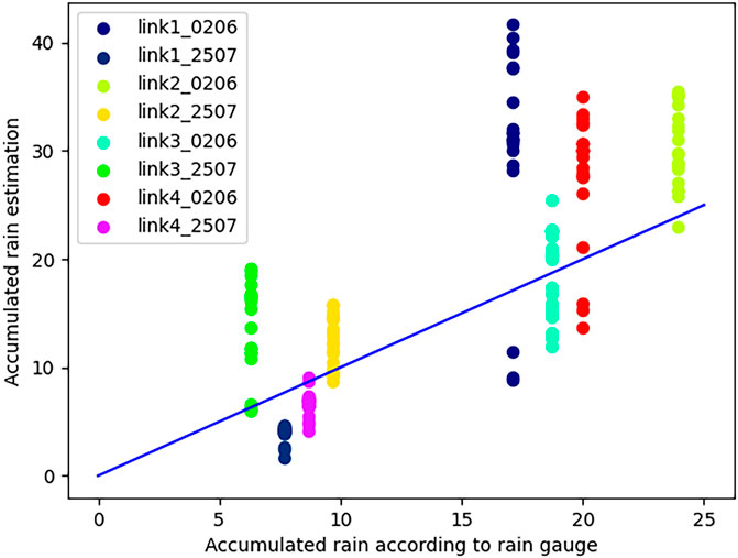
FIGURE 5. Accumulated rain estimation from the CMLs versus accumulated rain according to the rain gauge. Each group of points with the same color represents estimation based on one dual-channel link for different dates and varying window numbers, W. For each link, direction, and number of windows, the same averaged threshold was used for all dates.
3.3 Second experiment—the variance detector
In this experiment, we performed the detection using the variance detector from (1) and 8. We compare the accumulated rain estimation results when using our method for setting the detection threshold with the results obtained by the method for setting the threshold suggested in Schleiss and Berne (2010). In order to calculate the threshold based on the method in Schleiss and Berne (2010), we used attenuation measurements of dry periods during 12 days from the four CMLs in Gothenburg. We divided the dry-period attenuation measurement vectors to windows of 60 min and calculated the variance estimator for each window:
where
Figure 6 presents the accumulated rain estimation results when the threshold was set by the proposed minimum-risk method and by the reference method from Schleiss and Berne (2010) versus the ground-truth value of accumulated rain from the rain gauges. Each group of points represents the estimation from a single link for different dates, and the different points correspond to a varying number of windows and channels of the link. It can be seen that the estimation results obtained using the proposed method (denoted in Figure 6 by the “⋅” marker) fit the ground-truth values better than the estimation results obtained when setting the threshold using the reference method (denoted in Figure 6 by the “+” marker). When calculating the root mean square error (RMSE) of the accumulated rain estimation compared to the accumulated rain from the rain gauges, we received 6.9 mm using our method and 18.8 mm using the reference method. This demonstrative comparison implies that considering the accumulated rainfall estimation error during the detection stage can result in better total accumulated rainfall estimation compared to the conventional approaches in which the detection and estimation stages are decoupled.
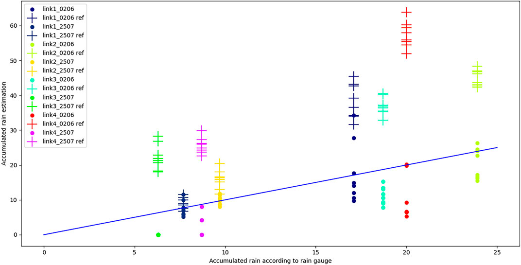
FIGURE 6. Accumulated rain estimation from the CMLs versus accumulated rain according to the rain gauge for the proposed method (.) and the reference method of 99% quantile of variance estimators in a dry period (+) (Schleiss and Berne, 2010).
4 Discussion and conclusion
In this study, we utilized the risk function suggested in Weiss et al. (2021) for the problem of post-detection accumulated rain estimation in order to set an optimal detection threshold. The considered risk used for the optimization penalizes both estimation and detection-related errors. Using actual measurements from operational CMLs and reference measurements from nearby rain gauges, we show that this approach significantly improves the accuracy of the accumulated rain estimation, relative to a method of setting the detection threshold based on the 99% quantile of the variance estimates over dry periods. We showed that the threshold that minimizes the empirical risk has good resemblance to the theoretical threshold that best matches the estimated accumulated rain with the value measured by the corresponding rain gauge.
In deriving the theoretical results, we assumed some simplifying assumptions as mentioned throughout the paper. Specifically, we assumed that the power law parameter b (of (10)) is equal to 1 and the rain is assumed to fall at a constant intensity within the short time window, and we ignore noise and interference components other than additive measurement noise. These assumptions are obviously not accurate, especially when using CMLs operating at high or low frequencies (for which 0.5 < b < 2 values are away from 1) and in locations where very strong and short bursts of rain are common. Nonetheless, as the empirical results show, practical robustness exists, and a deviation from the assumed approximations does not significantly change the results. However, future research may adapt the proposed approach to a more realistic rainfall model.
Lastly, it is worth noting that selecting the specific number of the effective size (i.e., the time-duration) of each window W (as described in Section 2) should be taken with consideration of the local climate in the area of interest. On the one hand, choosing a size W that is too long might reduce the accuracy if the rain variability changes significantly within each W; on the other hand, choosing W that is too short will result in fewer samples from which the risk is calculated, thus also negatively affecting the accuracy. In the experiment presented in this paper, we indeed show that a range of selected sizes of W all give similar outcomes. However, this might not be the case for different areas.
Future research can also focus on designing not only the detection threshold in a given estimation after detection scheme but also specific detection or estimation methods designated for accumulated rain that optimize the proposed joint detection–estimation risk. In addition, new performance bounds could be developed for this task, similar to the MSE bounds in post-model-selection estimation (Meir and Routtenberg, 2021; Nadav and Routtenberg, 2023).
Data availability statement
Publicly available datasets were analyzed in this study. These data can be found here: Andersson, J. C. M., Olsson, J., van de Beek, R. (C. Z. )., and Hansryd, J.: OpenMRG: Open data from Microwave links, Radar, and Gauges for rainfall quantification in Gothenburg, Sweden, Earth Syst. Sci. Data, 14, 5411–5426, https://doi.org/10.5194/essd-14-5411-2022.
Author contributions
TW: conceptualization, formal analysis, investigation, methodology, software, and writing–original draft. TR: conceptualization, supervision, validation, and writing–review and editing. JO: data curation, visualization, and writing–review and editing. HM: resources, supervision, validation, and writing–review and editing.
Funding
The author(s) declare that financial support was received for the research, authorship, and/or publication of this article. The work of TR has been partially supported by the Israel Science Foundation (Grant No. 1148/22).
Acknowledgments
The authors would like to thank their research team members from Tel Aviv University, Tel Aviv, Israel. They would also like to thank Dr. J. Hansryd and Dr. L. Bao from Ericsson AB, Sweden, who provided the real data.
Conflict of interest
The authors declare that the research was conducted in the absence of any commercial or financial relationships that could be construed as a potential conflict of interest.
The author(s) declared that they were an editorial board member of Frontiers at the time of submission. This had no impact on the peer review process and final decision.
Publisher’s note
All claims expressed in this article are solely those of the authors and do not necessarily represent those of their affiliated organizations, or those of the publisher, the editors and, the reviewers. Any product that may be evaluated in this article, or claim that may be made by its manufacturer, is not guaranteed or endorsed by the publisher.
Footnotes
1Setting each window to cover a full hour of measurements, excluding the last hour to ensure full alignment of the data
2It is worth noting the outlier in the results for link3 during the 2 June event. This anomaly might correspond with the fact that, in this case, the function has a number of local minima points, as is evident from the relevant plots in Figure 2.
References
Andersson, J. C., Olsson, J., Van de Beek, R., and Hansryd, J. (2022). OpenMRG: Open data from microwave links, radar, and gauges for rainfall quantification in Gothenburg, Sweden. Earth Syst. Sci. Data Discuss. 2022, 5411–5426. doi:10.5194/essd-14-5411-2022
Chaumette, E., Larzabal, P., and Forster, P. (2005). On the influence of a detection step on lower bounds for deterministic parameter estimation. IEEE Trans. signal Process. 53 (11), 4080–4090. doi:10.1109/tsp.2005.857027
Cherkassky, D., Ostrometzky, J., and Messer, H. (2013). Precipitation classification using measurements from commercial microwave links. IEEE Trans. Geosci. Remote. Sens. 52 (5), 2350–2356. doi:10.1109/tgrs.2013.2259832
Chwala, C., Gmeiner, A., Qiu, W., Hipp, S., Nienaber, D., Siart, U., et al. (2012). Precipitation observation using microwave backhaul links in the alpine and pre-alpine region of Southern Germany. Hydrology Earth Syst. Sci. 16 (8), 2647–2661. doi:10.5194/hess-16-2647-2012
Chwala, C., and Kunstmann, H. (2019). Commercial microwave link networks for rainfall observation: assessment of the current status and future challenges. Wiley Interdiscip. Rev. Water 6 (2), e1337. doi:10.1002/wat2.1337
D’Amico, M., Manzoni, A., and Solazzi, G. L. (2016). Use of operational microwave link measurements for the tomographic reconstruction of 2-d maps of accumulated rainfall. IEEE Geosci. Remote. Sens. Let. 13 (12), 1827–1831. doi:10.1109/lgrs.2016.2614326
Fencl, M., Dohnal, M., Valtr, P., Grabner, M., and Bareš, V. (2020). Atmospheric observations with e-band microwave links – challenges and opportunities. Atmos. Meas. Tech. 13 (12), 6559–6578. doi:10.5194/amt-13-6559-2020
Fencl, M., Rieckermann, J., Sỳkora, P., Stránskỳ, D., and Bareš, V. (2015). Commercial microwave links instead of rain gauges: fiction or reality? Water Sci. Technol. 71 (1), 31–37. doi:10.2166/wst.2014.466
Goldshtein, O., Messer, H., and Zinevich, A. (2009). Rain rate estimation using measurements from commercial telecommunications links. IEEE Trans. signal Process. 57 (4), 1616–1625. doi:10.1109/tsp.2009.2012554
Graf, M., Chwala, C., Polz, J., and Kunstmann, H. (2020). Rainfall estimation from a German-wide commercial microwave link network: optimized processing and validation for 1 year of data. Hydrology Earth Syst. Sci. 24 (6), 2931–2950. doi:10.5194/hess-24-2931-2020
Habi, H. V., and Messer, H. (2018). “Wet-dry classification using lstm and commercial microwave links,” in 2018 IEEE 10th sensor array and multichannel signal processing workshop (SAM) (IEEE), 149–153.
ITU-R.530 (2009). Propagation data and prediction methods required for the design of terrestrial line-of-sight systems. ITU-R 530-15.
ITU-R.838 (2005). Specific attenuation model for rain for use in prediction methods. ITU-R 838-3. 1992-1999-2003-2005.
Meir, E., and Routtenberg, T. (2021). Cramér-rao bound for estimation after model selection and its application to sparse vector estimation. IEEE Trans. Signal Process. 69, 2284–2301. doi:10.1109/tsp.2021.3068356
Messer, H., and Sendik, O. (2015). A New Approach to Precipitation Monitoring: a critical survey of existing technologies and challenges. IEEE Signal Process. Mag. 32, 110–122. doi:10.1109/msp.2014.2309705
Messer, H., Zinevich, A., and Alpert, P. (2006). Environmental monitoring by wireless communication networks. Science 312 (5774), 713. doi:10.1126/science.1120034
Nadav, H., and Routtenberg, T. (2023). Non-Bayesian post-model-selection estimation as estimation under model misspecification. ”arXiv preprint arXiv:2308.11359”. doi:10.48550/arXiv.2308.11359
Olsen, R., Rogers, D., and Hodge, D. (1978). The aR b relation in the calculation of rain attenuation. IEEE Trans. antennas Propag. 26, 318–329. doi:10.1109/tap.1978.1141845
Ostrometzky, J. (2017). Statistical signal processing of extreme attenuation measurements taken by commercial microwave links for rain monitoring. Ph.D. dissertation. Tel Aviv University.
Ostrometzky, J., Cherkassky, D., and Messer, H. (2015). Accumulated mixed precipitation estimation using measurements from multiple microwave links. Adv. Meteorology 2015, 1–9. doi:10.1155/2015/707646
Ostrometzky, J., and Messer, H. (2014). “Accumulated rainfall estimation using maximum attenuation of microwave radio signal,” in Sensor array and multichannel signal processing workshop (SAM), 193–196. doi:10.1109/SAM.2014.6882373
Overeem, A., Leijnse, H., and Uijlenhoet, R. (2013). Country-wide rainfall maps from cellular communication networks. Proc. Natl. Acad. Sci. 110 (8), 2741–2745. doi:10.1073/pnas.1217961110
Overeem, A., Leijnse, H., and Uijlenhoet, R. (2016). Two and a half years of country-wide rainfall maps using radio links from commercial cellular telecommunication networks. Water Resour. Res. 52 (10), 8039–8065. doi:10.1002/2016wr019412
Polz, J., Chwala, C., Graf, M., and Kunstmann, H. (2020). Rain event detection in commercial microwave link attenuation data using convolutional neural networks. Atmos. Meas. Tech. 13 (7), 3835–3853. doi:10.5194/amt-13-3835-2020
Rahimi, A., Holt, A., Upton, G., and Cummings, R. (2003). Use of dual-frequency microwave links for measuring path-averaged rainfall. J. Geophys. Res. Atmos. 108 (D15). doi:10.1029/2002jd003202
Schleiss, M., and Berne, A. (2010). Identification of dry and rainy periods using telecommunication microwave links. IEEE Geosci. Remote. Sens. Let. 7 (3), 611–615. doi:10.1109/lgrs.2010.2043052
Song, K., Liu, X., Zou, M., Zhou, D., Wu, H., and Ji, F. (2020). Experimental study of detecting rainfall using microwave links: classification of wet and dry periods. IEEE J. Sel. Top. Appl. Earth Observations Remote Sens. 13, 5264–5271. doi:10.1109/jstars.2020.3021555
Wang, Z., Schleiss, M., Jaffrain, J., Berne, A., and Rieckermann, J. (2012). Using Markov switching models to infer dry and rainy periods from telecommunication microwave link signals. Atmos. Meas. Tech. 5 (7), 1847–1859. doi:10.5194/amt-5-1847-2012
Weiss, T., Routtenberg, T., and Messer, H. (2021). Total performance evaluation of intensity estimation after detection. Signal Process. 183, 108042. doi:10.1016/j.sigpro.2021.108042
Keywords: accumulated rainfall estimation, commercial microwave links, detection threshold, opportunistic integrated sensing and communication, post-detection estimation
Citation: Weiss T, Routtenberg T, Ostrometzky J and Messer H (2024) Intensity estimation after detection for accumulated rainfall estimation. Front. Sig. Proc. 4:1291878. doi: 10.3389/frsip.2024.1291878
Received: 10 September 2023; Accepted: 08 January 2024;
Published: 07 February 2024.
Edited by:
Domenico Ciuonzo, University of Naples Federico II, ItalyReviewed by:
Gianluca Tabella, Norwegian University of Science and Technology, NorwayPia Addabbo, Giustino Fortunato University, Italy
Copyright © 2024 Weiss, Routtenberg, Ostrometzky and Messer. This is an open-access article distributed under the terms of the Creative Commons Attribution License (CC BY). The use, distribution or reproduction in other forums is permitted, provided the original author(s) and the copyright owner(s) are credited and that the original publication in this journal is cited, in accordance with accepted academic practice. No use, distribution or reproduction is permitted which does not comply with these terms.
*Correspondence: Hagit Messer, bWVzc2VyQGVuZy50YXUuYWMuaWw=