 Nayely Vélez-Cruz
- School of Electrical, Computer and Energy Engineering, School of Complex Adaptive Systems, Arizona State University, Tempe, AZ, United States
Time series analysis aims to understand underlying patterns and relationships in data to inform decision-making. As time series data are becoming more widely available across a variety of academic disciplines, time series analysis has become a rapidly growing field. In particular, Bayesian nonparametric (BNP) methods are gaining traction for their power and flexibility in modeling, predicting, and extracting meaningful information from time series data. The utility of BNP methods lies in their ability to encode prior information and represent complex patterns in the data without imposing strong assumptions about the underlying distribution or functional form. BNP methods for time series analysis can be applied to a breadth of problems, including anomaly detection, noise density estimation, and time series clustering. This work presents a comprehensive survey of the existing literature on BNP methods for time series analysis. Various temporal BNP models are discussed along with notable applications and possible approaches for inference. This work also highlights current research trends in the field and potential avenues for further development and exploration.
1 Introduction
Time series data collection has become increasingly prevalent in recent years across a range of industries, including finance, healthcare, and social media. The growth of cloud computing platforms has also facilitated the storage and processing of large and high-dimensional time series data. Time series analysis is thus becoming a rapidly growing field. Several challenges in this area include anomaly or change point detection, clustering multiple time series based on similar underlying patterns, and making predictions from time series with missing values or irregular sampling. To this extent, Bayesian nonparametric (BNP) methods are gaining traction for their power and flexibility in modeling, forecasting, handling missing values, and extracting meaningful information from time series data. The utility of BNP methods lies in their ability to encode prior information and represent complex patterns in the data without imposing strong assumptions about the underlying distribution or functional form. This makes them well-suited for a large range of time series problems where traditional models are too restrictive.
Bayesian nonparmetric methods center on the construction of statistical models over infinite-dimensional probability spaces. Unlike parametric methods, which assume a specific form for the underlying data distribution, BNP methods allow the model to learn from the data and adapt in complexity accordingly. BNP models use stochastic processes as their building blocks, the main ones being Dirichlet processes, Beta processes, and Gaussian processes. The rest of this work is organized as follows: In Section 2, I summarize the standard BNP models, how they are employed for various time series analysis problems, and highlight some important extensions. Section 3 centers on current state-of-the art developments, which focus on integrating BNP methods with deep learning for the analysis of high-dimensional data, as well as scaling these methods to large datasets. Section 4 highlights three areas for practical application: object tracking, healthcare and biomedical data analysis, and speech signal processing. I conclude by discussing some potential avenues for further exploration. Refer to Table 1 for the list of acronyms used throughout this work.
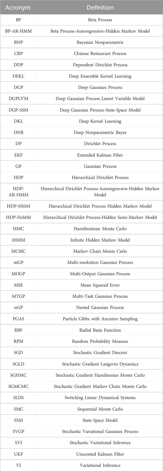
TABLE 1. Table of acronyms.
2 Standard nonparameric priors
2.1 Dirichlet processes and their extensions
At the core of BNP methods is the Dirichlet process (DP), which can be thought of as a probability distribution over the space of probability distributions. More formally, given a base distribution H over a measurable space Ω and a positive real number α, a random distribution
Extensions of the standard DP have been developed for problems in which the distribution of the observations is assumed to change in time, leading to several constructions of time-dependent DPs. These are well-suited for evolutionary clustering tasks, where the number of clusters and their associated parameters can vary with time (Caron et al., 2012; Ahmed and Xing, 2008; Ren et al., 2008; Zhu et al., 2005; Moraffah and Papandreou-Suppappola, 2022). The construction of time-dependent DPs is based on the dependent Dirichlet process (DDP), which is a stochastic process indexed by covariates such as space or time (Griffin and Steel, 2006). This construction can be done through Poisson processes (Campbell et al., 2013; Lin et al., 2010), stick-breaking (Campbell et al., 2013), or through Pólya urn and CRP (Caron et al., 2012; Ahmed and Xing, 2008). In a time-dependent DP, dependency is introduced between successive mixing distributions indexed by time t,
where Ft is an unknown pdf to be estimated and Θ is the set of latent parameters for the mixed pdf f (yt|θt). The random probability measure (RPM)
Note that
where k denotes the cluster index,
Time-dependency can be introduced through a stochastic process on the weights (Nieto-Barajas et al., 2012; Griffin and Steel, 2006), and/or atoms (Griffin and Steel, 2009). Note that in the construction in Eq. 3, time-dependency is introduced in both. In Mena and Ruggiero (2016), dependency is introduced on the weights by replacing the stick-breaking construction with a one-dimensional Wright-Fisher diffusion. Another diffusion process construction based on Fleming-Voit diffusion is introduced in Ascolani et al. (2021). In Rodriguez and Ter Horst (2008), dependency is introduced on the atoms through a dynamic linear model. In Lucca et al. (2013), dependency is introduced on the atoms through a simple linear autoregressive process, and an extension based on the Ornstein-Uhlenbeck process is developed. In Campbell et al. (2013), dependency is introduced on both the weights and atoms through a Poisson process construction. Although these approaches focus on discrete-time, an extension to the continuous time domain based on geometric stick-breaking processes is introduced in Mena et al. (2011), where dependency is introduced on the weights. These are summarized in Table 2.
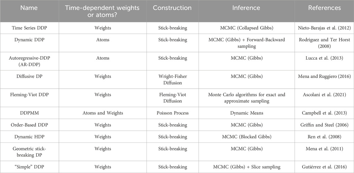
TABLE 2. Summary of time-dependent Dirichlet processes based on the stick-breaking construction. Time-dependency on the weights and/or atoms, the specific construction, and inference algorithm are listed. See reference associated with each model for more details.
Many constructions of time-dependent DPs are based on the Pólya urn scheme or the CRP, which facilitate efficient inference (Caron et al., 2012; Ahmed and Xing 2008; Zhu et al., 2005; Blei and Frazier, 2011). It is important to note how the cluster assignment probabilities are computed in these various methods. Time-dependency alters the standard formulas for calculating the probabilities of assigning new data to a cluster, as they become dependent in some way on the number of times a cluster has been chosen at previous time points. For example, the model may take into account the entire history’s cluster assignments for t = 1: t − 1 (Caron et al., 2017; Caron et al., 2012), the previous time point’s (t − 1) assignments (Özkan et al., 2011; Ahmed and Xing, 2008), or be based on some other metric (Saad and Mansinghka, 2018). These are summarized in Table 3. In Zhu et al. (2005), the authors develop a time-sensitive DP model for time-varying topic modeling. They introduce a decaying exponential weight function into the probabilities of assigning data to a cluster which incorporates the entire history of previous cluster assignments. This model is quite flexible as it allows different clusters to have different decay rates and can capture different types of dynamic behavior such as periodicity, but it is not consistent under marginalization. In Ahmed and Xing (2008), the authors introduce a time-dependent DP based on the recurrent CRP. This approach assumes that the data arrive in T consecutive epochs, where data in the same epoch are assumed to be fully exchangeable and there are an infinite number of clusters in each epoch. The cluster assignment probabilities are computed by taking into account the previous epoch’s (t − 1) cluster assignments and the number of points already assigned to the cluster in the current epoch rather than the entire previous history. An advantage of this approach is that it captures time-varying cluster popularity. Other notable works include the distance dependent CRP, which captures the property that data points which are closer in time are more likely to cluster together (Blei and Frazier, 2011). The model introduced in Ren et al. (2008) also exhibits this property while simultaneously allowing the possibility of repetition, as temporally distant data may share parameters. Many of these time-dependent DPs also allow clusters to stay, re-emerge, and die out over time (Caron et al., 2017; Lin et al., 2010). These dynamics can be incorporated through a cluster removal step as in Caron et al. (2017), Caron et al. (2012), which has been used for time-varying density estimation (Jaoua et al., 2014; Rodriguez and Ter Horst, 2008).
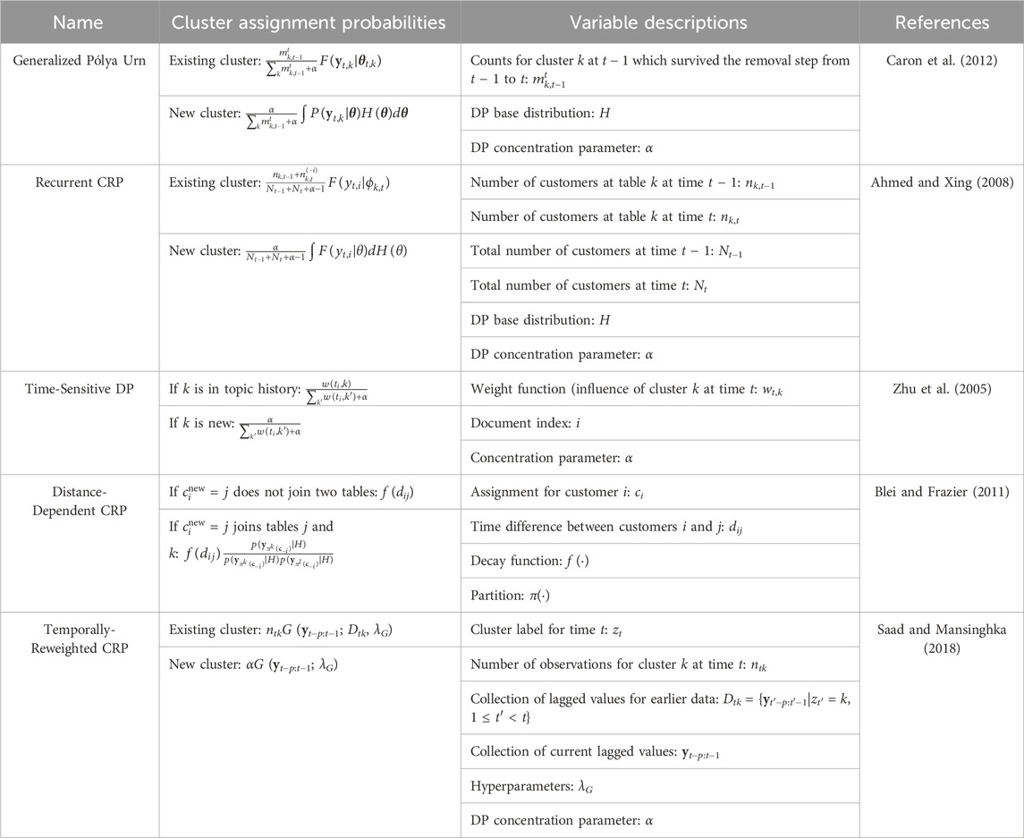
TABLE 3. Summary of time-dependent Dirichlet processes based on the Pólya urn or CRP constructions. Note the differences in computing the cluster assignment probabilities.
Of particular note are more recent works which focus on clustering multiple time series exhibiting similar behaviors. In Lin et al. (2019), the authors introduce the DP nonlinear State-Space Mixture (DPnSSM), which clusters multiple time series which exhibit nonlinear dynamics. By placing DP priors over the unknown parameters in the nonlinear transition dynamics, the model induces clustering of the time series based on their specific dynamics. Similar work by Nieto-Barajas and Contreras-Cristán (2014) employs a Poisson-Dirichlet process mixture model which can use trends, seasonality, or temporal components as a basis for clustering. Interestingly, Saad and Mansinghka (2018) introduce a temporally re-weighted CRP and a hierarchical extension for forecasting, missing data imputation, and clustering multivariate time series. Their approach identifies similar segments within individual time series, and is then used to cluster hundreds of time series into groups, where each group’s underlying dynamics are modeled jointly. Several approaches for specifically clustering biological time series have also been developed. In McDowell et al. (2018), the authors use a DP mixture of Gaussian processes to cluster gene expression time series. A Gaussian process prior, which will be discussed in depth in Section 2.2, is placed over the unknown transition dynamics while the DP allows clustering of gene expression time series data based on these dynamics. In Yu et al. (2016), fetal heart rate signals are clustered using the hierarchical Dirichlet process (HDP), which facilitated the identification of clusters specific to diseased and healthy fetuses. Overall, these methods have been successful in identifying shared features in multiple time series across a variety systems and have been applied to a diverse range problems including multiple object tracking, evolutionary topic modeling, and video segmentation (Neiswanger et al., 2014; Moraffah et al., 2019; Srebro and Roweis, 2005; Barker and Davis, 2014).
2.1.1 Hidden markov models
An important extension of the Dirichlet process for the analysis of time series data is its application to Hidden Markov Models (HMMs). Unlike the traditional HMM, which requires the number of hidden states to be specified a priori, incorporating a DP prior on the state transition dynamics provides a distribution over an infinite number of states. This allows the number of hidden states to be learned directly from the data. The HDP-HMM and its extensions have a range of applicability, including speech recognition, image segmentation, and genomics (Fox et al., 2011b; Teh and Jordan, 2010; Yau et al., 2011). A summary of these models is given in Table 4.
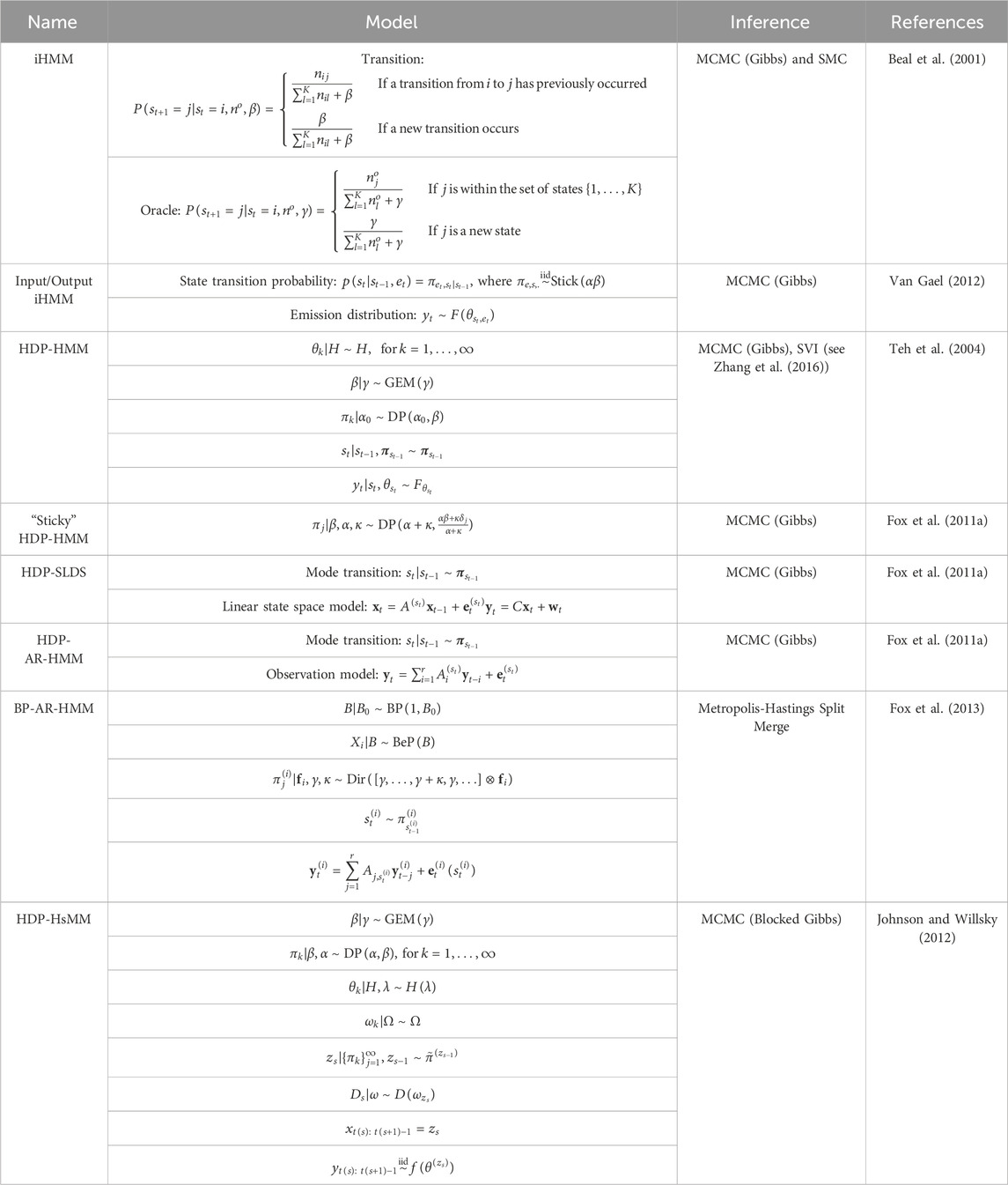
TABLE 4. Summary of Bayesian nonparametric HMMs. See reference associated with model of interest for more information.
2.1.1.1 Infinite hidden markov model (iHMM)
One early development is the infinite hidden Markov Model (iHMM) (Beal et al., 2001), which uses a two-level DP to model the state transition dynamics (the transition probabilities for each row of the transition matrix). The iHMM is constructed via a coupled set of Pólya urns. Specifically, the transition from state st to st+1 is modeled as a DP with concentration β according to Eq. 6:
where nij is the number of transitions from state i to j. Novel transitions occur with a finite probability
A prior mass α is used to control the probability of self transitions. To complete the model, parameters θk for the emission distribution corresponding to each state k are drawn from a base distribution H and the likelihood is given as
2.1.1.2 Hierarchical Dirichlet process-hidden markov model (HDP-HMM)
An alternative construction is the Hierarchical Dirichlet Process-Hidden Markov Model (HDP-HMM) (Teh et al., 2004). In an HDP-HMM each row in the transition probability matrix corresponds to a draw from an HDP where an HDP prior is used over an infinite state space. This allows outgoing states to share transitions into the same set of states. The generative model is constructed via stick-breaking and the hierarchy is given by Eqs 8–12 as follows.
Where H is the HDP base distribution,
2.1.1.3 “Sticky” HDP-HMM and extensions
Influential work by Fox et al. (2011a) extended the HDP-HMM to capture state persistence, known as the “sticky” HDP-HMM (Eq. 13). It is given by
where the parameter κ captures state persistence by increasing the probability of self-transition. The sticky HDP-HMM prior allows the dynamical model to switch between an unknown number of states while preventing the model from switching too quickly between redundant states. Two extensions of the “sticky” HDP-HMM were introduced in Fox et al. (2011a) to learn switching linear dynamical systems, where each state in the HMM is associated with a linear dynamical model. The first is the HDP-Autoregressive-HMM (HDP-AR-HMM), which places an HDP prior on the mode-specific matrices
where et is the noise vector and the mode dynamics are given by
Where wt is the observation noise and C is the measurement matrix. Again, the mode dynamics are given by
2.1.1.4 Beta process-autoregressive HMM (BP-AR-HMM)
An issue with the HDP-HMM arises when applied to the analysis of multiple time series in that it assumes that all time series sequences share the same sets of states. To address this problem and to increase the flexibility of these methods, another type of Bayesian nonparametric HMM has been developed using the Beta process (BP), referred to as the Beta Process-Autoregressive HMM (BP-AR-HMM) (Fox et al., 2013). Note that the Beta process is used as a nonparametric prior over latent binary feature matrices. This construction captures shared dynamical behaviors across multiple time series and indicates which behaviors are exhibited by each time series (Fox et al., 2013). The hierarchical model is given by Eqs 17–21:
Where the global weights are provided by B, which is a draw from a Beta Process (BP), and Xi is a realization of a Bernoulli process such that
2.1.1.5 HDP-hidden semi-markov model (HDP-HsMM)
In the standard HDP-HMM and “sticky” HDP-HMM, the state durations are geometrically distributed and the self-transition parameter is shared across all states. These assumptions are not suitable for situations where we may want to capture bimodal or multimodal state distributions. For instance, in modeling the behavior of consumers in a shopping mall, some users might briefly check something and leave, while others might spend a long time browsing. An alternative to the “sticky” HDP-HMM is the HDP-Hidden Semi-Markov Model (HDP-HsMM), which incorporates explicit duration semi-Markovianity by placing a distribution over the state duration (Johnson and Willsky, 2012). Once the state is reached, a duration time is drawn from the duration distribution and the system stays in the state until the duration period ends before transitioning to a new state. Let
Where wk are duration distribution-specific parameters for each state k = 1, … ∞,
2.2 Gaussian processes
Another set of fundamental BNP methods for analyzing time series data is based on the Gaussian process (GP). The GP is formally defined as a potentially infinite collection of random variables such that the joint distribution of any finite subset is a multivariate Gaussian. It is used as a prior over unknown functions. A draw from a GP is denoted as f(x) ∼GP(mf(x), kf(x, x′)), where
The posterior mean and covariance are given by Eqs 31, 32:
One of the key strengths of GPs is in their ability to incorporate prior knowledge about a range of interesting dynamics, such as change points, periodicity, delays, long and short-term dynamics, smooth variation and more (Roberts et al., 2013; Saad et al., 2023). Moreover, they are suitable for handling missing data, modeling errors, quantifying uncertainty, and tend to be more robust to overfitting, making them a powerful tool. Some notable uses of GPs in the realm of time series analysis are for system identification in state-space models (SSMs), where the GP is used as a prior over the transition dynamics and/or measurement function. This is a particularly challenging problem because the unknown transition function depends on the unknown state at time t. In general, for unknown states xt at time t, measurements yt, and unknown transition functions f, the state space formulation is given by the following hierarchy in Eqs 33–35:
Where wt−1 and vt are typically additive Gaussian noise terms for the process and measurement dynamics, respectively. Several works have tackled the system identification issue using different strategies (Eleftheriadis et al., 2017; Frigola et al., 2013; Frigola et al., 2014). In Deisenroth et al. (2012), the authors introduce a novel method for computing a Gaussian approximation to the smoothing distribution referred to as the Rauch-Tung-Striebal (RTS) smoother, which outperforms popular smoothing algorithms such as the extended Kalman filter (EKF) and unscented Kalman filter (UKF). In Frigola et al. (2013), the authors introduce a multi-step approach which involves marginalizing out the unknown function f and drawing a sample from the smoothing distribution using particle Gibbs with ancestor sampling (PGAS). Thus, the unknown states can be sampled from the smoothing distribution without knowledge of the transition function. Follow-up work in Frigola et al. (2014) introduces a more efficient learning approach based on variational sparse GPs, which reduces the computational complexity to be linear in the length of the time series, making it faster to compute predictions of future trajectories. As well, GP approaches have been shown to effectively predict chaotic time series (Petelin and Kocijan, 2014). In Aalto et al. (2018); McDowell et al. (2018), GPs were used to infer underlying dynamics which were then used as a basis for clustering gene regulatory network time series.
Although appealing, one drawback of these methods is that they suffer from scalability issues, making them unsuitable for large and high-dimensional datasets. However, methods for improving scalability will be discussed in Section 3.4. As well, GPs cannot model multimodal or heavy-tailed marginal distributions. This can make them less robust to outliers and results in less accurate uncertainty estimates. Instead, a Sudent’s-t process may be more appropriate for such situations (Tracey and Wolpert, 2018), which has an extra parameter controlling the kurtosis of the distribution. Lastly, the expressivity of GPs is limited by the choice of kernel, making them unsuitable to learn complex relationships or features from time series data. An alternative to these last two issues is to use a deep learning BNP approach, which can equip GPs with the power to learn complex representations from data. This will be discussed in Section 4.1.
2.3 Multi-output GPs
Standard GPs, also called single-output GPs, model a single output variable as a function of input variables. A useful extension of GPs is the multi-output GP (MOGP), where an input or set of inputs can have multiple correlated outputs. For example, in a healthcare scenario, changing the drug dosage may have an affect on heart rate, blood sugar, and cholesterol levels. In such a scenario, the MOGP would model each output (heart rate, blood sugar, and cholesterol levels) jointly. The joint modeling leads to better predictive performance compared to single-output GPs. As well, sharing information between outputs typically reduces overfitting and is particularly useful when some outputs have limited data. To construct an MOGP, one just needs to specify a covariance kernel over the outputs in addition to one over the inputs. For k = 1, … , K outputs, the joint prior is given by Eqs 36, 37:
where in general, the covariance kernel in Eq. 38 is given by the following multiplication of two separable kernels (Eq. 39):
The regression model is specified as follows
The model in Equation 40 can easily be extended to time series through the addition of a time index as yk,t = fk (xt) + ϵk,t. Note that the covariance function takes into account correlations between inputs x and x′ as well as correlations between outputs k and k′. Through the construction of the covariance kernel, it is possible to simultaneously capture a range of underlying structures. In general construction can be as straightforward as adding or multiplying two or more separable kernels (e.g., multiplying a periodic kernel by a squared exponential kernel), or can be done through coregionalization models in which one defines a matrix B where entry (i, j) describes how outputs i and j are correlated with each other (Liu et al., 2022a). In addition to leveraging information from more data-rich outputs to help inform other data-poor outputs, MOGPs can also be applied to problems involving heterogeneous outputs (e.g., continuous, binary, and categorical) (Moreno-Muñoz et al., 2018). As well, they have been applied to multi-fidelity datasets with multiple correlated outputs (Lin et al., 2021). Unfortunately, the computational complexity of MOGPs is
2.3.1 Multi-task GP
A notable application of MOGPs is to multi-task learning. In multi-task learning, the objective is to improve the performance of multiple related learning tasks by pooling the information across the different tasks (Bonilla et al., 2007). The underlying assumption is that the tasks are not completely independent and can benefit from the knowledge contained in one another. It should be distinguished from transfer learning, which aims to use the knowledge gained from one or more source tasks to help learn a different, but related target task. In contrast, multi-task learning aims to improve the learning of multiple related tasks by learning them simultaneously, allowing the model to leverage shared information across the tasks. Multi-task learning therefore focuses on the identification of shared structures, making it suitable for multivariate time series analysis. Bayesian nonparametric methods for multi-task learning leverage the power of Gaussian processes to extract knowledge from multiple related time series, resulting in the multi-task GP (MTGP).
The key concept underlying the MTGP is the construction of a multi-task covariance kernel, which characterizes the correlation within and between tasks. This proceeds in the same manner as in a MOGP, except that each output k is now a task. Although better able to capture rich structures in data compared to standard GPs, these methods suffer from a few drawbacks. First, it is assumed that all tasks are equally important which may not be the case in real-world applications. Furthermore, these methods are computationally intensive due to the large number of parameters involved, as the covariance matrix associated each task or time series will have its own set of hyperparameters. Lastly, the complexity associated with the inversion of the covariance matrix makes it unsuitable for large and high-dimensional time series data. To address these issues, recent work has focused on developing deep learning paradigms with sparse inference methods for BNP multi-task learning, which will be discussed in Section 3.
2.3.2 Multi-resolution GP
Many real-world problems involve the analysis of data collected from different sources with varying resolutions or where the underlying phenomenon may have spatial and/or temporal multi-scale features. For example, EEGs may exhibit long-term patterns relating to circadian rhythms, but abrupt changes or sharp spikes may also be present due to a seizure. A limitation of standard GPs is that although they can capture long-range dependencies and sudden changes, they cannot do so simultaneously. To address this limitation, the multi-resolution GP (mGP) was introduced Fox and Dunson (2012), which is constructed by coupling a collection of smooth GPs in a hierarchical manner. Each GP is defined over an element of a nested partition
where ci is the covariance function. Recent work in Longi et al. (2022) applied the mGP framework to model the effects of multiple time scales in GP-SSMs, which can capture slow and fast transitions. mGPs have also been extended to the multi-task setting in Hamelijnck et al. (2019).
2.4 Posterior inference
Approaches for posterior inference are based on Markov Chain Monte Carlo (MCMC) or variational inference (VI). MCMC methods are asymptotically exact, but can be slow and difficult to scale, particularly in high-dimensional settings. The most commonly-used MCMC method is Gibbs sampling, which iteratively samples from the conditional distributions of the variables of interest and constructs a Markov chain whose stationary distribution is the target posterior distribution. In contrast, VI is an optimization-based approach, which seeks the distribution within the chosen variational family that is closest to the true posterior, as measured by the Kullback-Leibler (KL) divergence. VI is scalable to large datasets but can be more prone to approximation errors as the accuracy depends on the choice of the variational family. A stochastic extension of VI (SVI) is often used in conjunction with sparse Gaussian processes for scalability to large datasets. This section discusses both classes of methods. Table 5 provides references for the reader to further explore inference methods associated with their model of interest.
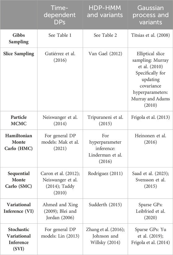
TABLE 5. Summary of inference approaches available for the three classes of BNP models.
2.4.1 Markov chain Monte Carlo (MCMC)
Markov Chain Monte Carlo (MCMC) methods generate samples from a target posterior distribution
2.4.2 Stochastic gradient MCMC (SGMCMC)
Stochastic Gradient MCMC (SGMCMC) presents a scalable alternative to standard MCMC methods by using noisy gradient estimates obtained from mini-batches of the data. Two such methods are stochastic gradient HMC (SGHMC) and stochastic gradient Langevin dynamics (SGLD), which introduce noise to the gradient computations of the log-posterior densities. In SGLD, Langevin dynamics are introduced into the standard stochastic gradient descent (SGD) and the parameters are updated by adding a Gaussian noise term (Nemeth and Fearnhead, 2021). The trajectory of the parameters resembles the behavior of particles undergoing Brownian motion as described by Langevin dynamics. As the name suggests, SGHMC is a stochastic extension of HMC. In Chen et al., (2014), a friction term is added to the momentum update to ensure that the Hamiltonian dynamics have the target distribution as the invariant distribution as simply injecting the noise to the gradient results in the target distribution no longer being the invariant distribution. The addition of the friction term thus stabilizes the Hamiltonian dynamics. An advantage of SGLD over SGHMC is that it is typically easier to implement and requires tuning fewer hyperparameters. However, since SGLD lacks the momentum component present in SGHMC, SGLD may be less efficient in exploring the parameter space in high-dimensional settings (Chen et al., 2014).
2.4.3 Optimization-based inference
Optimization-based methods, such as VI and stochastic variational inference (SVI), are often faster and outperform MCMC on large datasets at the expense of precision. The main idea underlying standard VI is to posit a family of simpler, tractable distributions (known as the variational family) and then find the member of this family that is closest to the target distribution (Blei et al., 2017). Optimization is performed through coordinate ascent or gradient descent on the entire dataset, making it computationally intensive for large datasets, although parallel VI is discussed in Campbell et al. (2015). In contrast, SVI operates similarly to SGMCMC by computing noisy estimates of the gradient on mini batches of the data, thereby making it more computationally efficient and well-suited to online settings. As in SGMCMC, the added stochasticity aids the model in escaping local optima. However, compared to VI, the added noise in SVI can lead to more errors. As well, the accuracy is influenced by the choice of minibatch size and the specific choices of the minibatches themselves may result in biased estimates.
2.5 Concluding remarks
Standard BNP approaches based on Dirichlet processes, Gaussian processes, and their most widely used extensions constitute a powerful statistical toolkit for a diverse range of time series analysis problems, such as within- and across-time series clustering, inferring unknown transition dynamics, and identifying change points in switching systems. As large and high-dimensional time series are becoming increasingly prevalent, more sophisticated approaches are needed to extract complex features and relationships from such data. The next section highlights some ongoing research trends in this regard as well as potential avenues for further exploration.
3 Current research trends
Although this work has highlighted several advantages of BNP methods for time series analysis, significant challenges still remain when analyzing both large and high-dimensional time series data that coalesce around the “curse of dimensionality”. This manifests in local kernel methods, such as the GP, as local kernels degenerate to one-nearest-neighbor classifiers in high dimensions (Agrawal, 2020; Bengio et al., 2005). As well, due to the lack of expressivity of the kernels, GPs lack the power to learn complex and abstract representations from high-dimensional datasets and instead act as smoothers (Ober et al., 2021). Dirichlet processes also face certain challenges in high-dimensional settings. Clusters may be more difficult to identify in high dimensions as distances between points become increasingly homogeneous and not all dimensions may be informative for clustering. Density estimation in high-dimensions also presents a challenge as large amounts of data are required to obtain meaningful estimates. In regard to inference, standard MCMC approaches also suffer from the “curse of dimensionality”, as data in high-dimensional settings can be sparse so the rate of convergence tends to decrease with an increase in dimension (Nagler and Czado, 2016). To address these challenges, current research trends center on the development of BNP deep learning methods for large and high-dimensional data. Integrating deep learning architectures and BNP methods enables the models to learn sophisticated representations of data which can improve predictions, provide reliable uncertainty estimates, and reduce the overfitting which deterministic neural networks are prone to. Sections 3.1 and 3.2 highlight two approaches: deep kernel learning (Wilson et al., 2016a; Al-Shedivat et al., 2017) and deep Gaussian processes (Damianou and Lawrence, 2013). However, an increase in model complexity necessitates computationally efficient methods. To this extent, another area of ongoing research centers on the development of scalable inference for BNP deep learning models, which will be discussed in Section 3.4.
3.1 Deep kernel learning
Pivotal research by Neal (1996) has demonstrated an important theoretical connection between GPs and neural networks, which is that infinitely wide neural networks converge to a GP. This result also extends to deep neural networks (Lee et al., 2017). His work provides a theoretical basis for which neural networks and GPs can be interwoven. Deep kernel learning (DKL) is one such manifestation. In DKL, a deep learning neural network is used as the kernel function of a GP. The neural network transforms high-dimensional inputs into a lower dimensional feature space representation where these features become an input into a GP. This confers a model with both of the advantages of GPs and neural networks: quantifying uncertainty and learning complex abstract representations. Equation 42 defines a deep kernel as follows:
where
DKL has recently been applied to the discovery of dynamical models and latent states from high-dimensional noisy time series data (Botteghi et al., 2022). In Botteghi et al. (2022), an encoder is used to compress high-dimensional measurements into low-dimensional state variables and SVI is used for learning. The efficacy of this model was demonstrated through learning the stochastic motion of a pendulum with external perturbations from high-dimensional noisy images. Although not specifically DKL, a related method from the image processing community integrates DP clustering with deep learning neural networks. In Wang et al. (2022), the authors develop Deep Nonparametric Bayes (DNB) for jointly estimating the number of clusters, cluster labels, and learning deep representations in image data. This is done by first passing the images through a convolutional neural network, then performing DP clustering on the features. These methods have also been applied to the development of deep factor analysis models (Mittal et al., 2020) and deep tracking models (Zhang and Paisley, 2018). An interesting possible application is to time series image data, which may be useful in biomedical applications, for example, in grouping heterogeneous cancer patient populations in subpopulations based on the progression of their cancer type.
3.2 Composite models: Deep vs. nested
Another set of approaches centers on the construction of deep Gaussian processes. The term “deep” is used rather inconsistently in the literature to refer to several different nested or composite extensions of standard Bayesian nonparametric models with deep architectures. These research areas are fairly new, so there has not yet been sufficient time to develop a standardized language. Based on the analysis of the literature, it was found that there are two terms used to refer to GPs with deep architectures: nested Gaussian processes (nGPs) and deep Gaussian processes (DGPs). In an nGP, or more generally any nested BNP model, the hyperparameters of the model are drawn from another BNP model. In the case of an nGP, for example, the mean function or the hyperparameters of the covariance kernel of a GP are themselves drawn from a GP prior. Similarly, the atoms of a nested Dirichlet process (nDP) are themselves draws from a DP. The term DGP is used more broadly. According to Damianou and Lawrence (2013), a DGP is a multi-layer network consisting of GPs, where the input of each GP is the output of another GP. Intriguingly, the literature on DGPs also contains several works which use an nGP model but refer to it as a DGP (Zhao, 2021; Zhao et al., 2021; Lu et al., 2020). Adding to the convolution, nGP-centric papers do not reference DGP studies and vice versa, obscuring the distinct dependencies each model encapsulates. Per the definition in Damianou and Lawrence (2013), the DGP model refers to a cascade of transformations on the input in which one GP feeds its output into another GP. This introduces a state or sequence-specific dependency in the model structure based on direct input/output relationships. In contrast, nGPs or other nested BNP models exhibit behavior-specific dependency. For example, in an nGP, the behavior of the primary predictive GP at a specific input point is influenced by the hyperparameters at that input. Instead of the hyperparameters being static, they are dynamically modeled by another GP. This allows them to vary across the input space, resulting in heightened flexibility and adaptability in comparison to standard GPs with unchanging hyperparameters. To enhance conceptual clarity, I will refer to DGPs defined in Damianou and Lawrence (2013) as sequence-dependent DGPs, while nGPs and DGPs built upon the nGP foundation will be designated as behavior-dependent DGPs. This choice of nomenclature retains the inherent deep architecture of both models but underscores the unique dependencies each encapsulates. I will continue using the term “nested” for non-GP nested BNP models.
3.2.1 Sequence-dependent DGPs
Although there are several ways to construct a sequence-dependent DGP (Dunlop et al., 2018), this work highlights construction via composition since it provides the most intuitive understanding of the architecture. A sequence-dependent DGP consists of three types of nodes: parent latent node Z, intermediate latent space nodes Xh−1, and leaf nodes Y (Teng et al., 2018). The parent latent node represents the initial input of the DGP. The intermediate latent node corresponds to h = 1, … , H − 1, where H is the number of hidden layers. The leaf node Y represents observed output, or target variables of the model. The graphical model in Figure 1 depicts the architecture for H hidden layers.
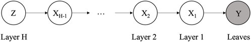
FIGURE 1. Graphical model representation for the deep Gaussian process adapted from Salimbeni and Deisenroth (2017). The output of each layer becomes the input into the next layer.
The generative process is given by Eqs 43, 44:
where the joint posterior is given in Eq. 45:
Note that a temporal extension (Eqs 46–49) can be formulated as follows:
Where independent GP priors are placed over the functions corresponding to each layer
Although there are few applications of sequence-dependent DGPs to the analysis of time series data, recent work by Chen et al. (2020) developed a sequence-dependent DGP approach to predict flight trajectories. They found that the ability of the sequence-dependent DGP to represent nonlinear features helped improve prediction accuracy as it could better capture flight environment stochasticity. Other work has extended sequence-dependent DGPs to state-space models (DGP-SSM) (Eq. 50) (Liu et al., 2022b; Taubert et al., 2022; Zhao, 2021). The formulation is given as
where ϵL,t is the error term corresponding to the Lth layer at time t, g is the possibly unknown measurement function, fl is the function mapping xl−1,t to xl,t, and f0 is the transition function mapping the state x0,t−1 at time t − 1 to the state x0,t at time t. In Liu et al. (2022b), the authors consider a DGP-SSM where both the state transition and measurement functions are assumed unknown. To induce sparsity, a feature-based representation of the GPs is used. An SMC algorithm is developed for inference on a simulated dataset consisting of two hidden layers, a five-dimensional measurement, and two-dimensional state vector. How this type of SMC algorithm scales to high-dimensional and large time series data remains an open question. To this extent, Taubert et al. (2022) introduce a computationally efficient algorithm combining sparse GPs and stochastic expectation propagation for inference in DGP-SSMs. The algorithm was evaluated on kinematic data with 99 degrees of freedom and was shown to outperform the standard GP dynamical model in terms of prediction accuracy via mean squared error (MSE). Comparison to other comparable methods such as DKL is needed to fully evaluate the efficacy of their approach, but this is an exciting area for future research.
3.2.2 Behavior-dependent DGPs and nested BNP models
In a behavior-dependent DGP (Eq. 51), a GP prior is placed on the parameters of a GP, such as the mean function or the hyperparameters of the covariance kernel (Zhao et al., 2021). Like the sequence-dependent DGP, this layering can continue indefinitely. An example of such a construction is given by
where t and p correspond to different levels of nesting and the mean of ft, which is μt is drawn from a GP. Although sequence and behavior-dependent DGPs can model complex relationships between data in a hierarchical manner, they offer different advantages. In particular, the behavior-dependent DGP construction allows for explicit modeling of non-stationary behavior as the GP parameters are allowed to vary across the input space. Non-stationarity is inherent in its construction. In contrast, sequence-specific DGPs typically implicitly model non-stationarity through the successive nonlinear transformations of the input. However, non-stationarity can also be introduced in the kernel construction. Incorporating behavior-dependent DGPs in a state-space model framework enables us to capture several levels of spatial and/or temporal granularity in the dynamics. By allowing a GP to modulate the parameters of another GP, they can adapt very locally to data. This makes them well-suited for modeling data with rapid fluctuations or change points, varying scales of trends, or input region specific patterns and have the ability to model a larger class of functions (Zhao et al., 2021). Behavior-dependent DGPs have exhibited success in imputing missing data in high-dimensional settings while modeling complex spatiotemporal relationships in healthcare settings (Imani et al., 2019).
Other related methods are based on nested partition models (Mansinghka et al., 2016), such as nested Dirichlet processes (nDPs, Eqs 52–55) (Rodríguez et al., 2008), which can be used to cluster entire distributions. The hierarchical model for the nDP is given as
Which admits the stick-breaking construction in Eq. 56
and
Note that Q in Eq. 57 is defined as an infinite-dimensional distribution over all possible DPs. With probability πr, a DP Gr is selected which sets Gj = Gr. This allows clustering of the distributions themselves. A marginalized nDP based on the Pólya urn construction is introduced in Zuanetti et al. (2018). Unfortunately, the nDP can degenerate to the fully exchangeable case if two populations share at least one latent variable (Camerlenghi et al., 2019). More recently, a latent nested partition model was introduced in Camerlenghi et al. (2019) to overcome the degeneracy issue of the nDP. An open area of research is the development of temporal extensions of these nested partition models to allow for time-varying distributional cluster membership, which may be more reflective of the dynamic nature of real-world populations.
3.3 Deep Gaussian process multi-task learning
Extending DGPs to multi-task settings results in powerful models equipped with the advantages of MTGPs and the ability to learn complex relationships and patterns in data. An advantage of incorporating a deep architecture in an MTGP model is that it is less sensitive to the specific form of the covariance kernel, which is not the case in standard GP or MTGP analysis. The deep architecture helps mitigate this sensitivity, making the model more robust and adaptable to various types of data. Deep architectures also provide increased expressivity. This is especially advantageous when handling tasks characterized by intricate and nonlinear dependencies. Such complexities may pose challenges for shallower models (Boustati et al., 2020; Boustati and Savage, 2019). Deep MTGP models not only maintain the ability to provide informative uncertainty quantifications but also uphold robustness against overfitting. Moreover, the hierarchical representation and feature learning capabilities of DGPs contribute to better generalization across tasks. The model can leverage shared features and representations to make predictions on new or unseen tasks, promoting more effective transfer of knowledge between related tasks.
3.4 Posterior inference scaling to large datasets
Many of the approaches just discussed are computationally intensive and require methods to scale to large datasets. Although it is important to note that GP inference in general admits parallelization and distributed inference (Agrawal, 2020), one should exercise caution when dealing with time series data which exhibit strong dependencies or high correlations so that the integrity of the temporal dependencies is maintained. Stochastic variational inference algorithms for GPs have been successfully applied to large datasets (Hensman et al., 2013) and provide a path for scaling deep learning BNP methods to large and high-dimensional datasets (Hoffman et al., 2013). One recent approach is the use of sparse variational Gaussian processes (SVGPs). SVGPs reduce the computational complexity of a standard Gaussian process from
4 Practical applications
Bayesian nonparametric (BNP) methods showcase versatility in numerous domains. This section highlights their diverse applications in three areas, specifically focusing on object tracking, healthcare and biomedical data analysis, and speech signal processing.
4.1 Object tracking
Object tracking aims to locate and follow the movement of objects captured by a sensor, such as radar, GPS, or a camera over time. Unlike traditional methods that assume a fixed number of objects or rely on predefined detection models, Bayesian nonparametric methods allow for flexibility in handling varying object counts and diverse types of objects, as well as adapting to varying environments (Moraffah et al., 2020). In Fox et al. (2006), the authors consider the problem of multiple-object tracking when the number of objects is unknown. This involves assigning measurements collected by a sensor to their underlying targets. Using a linear state-space model to model the dynamics of each target and measurement, a Dirichlet process (DP) prior is placed on the number of targets. Gibbs sampling is used to infer the target-measurement associations and identify 10 targets based on their measurement trajectories. In Caron et al. (2012); Neiswanger et al. (2014), a time-dependent DP construction based on the generalized Pólya urn scheme is introduced to track multiple objects in videos. Each object is modeled as a multiplication of a multivariate Gaussian and multinomial distribution to capture its location and RGB color distribution. A dependent Dirichlet process (DDP) prior is placed on the set of parameters corresponding to these distributions, which allows the model to capture a range of object shapes and orientations (Neiswanger et al., 2014). Using a variety of inference algorithms including particle Gibbs and sequential Monte Carlo (SMC) with a local Gibbs step, the authors apply their method to three scenarios. The first is a video containing six ants exhibiting erratic behaviors where the video background is a similar color scheme to the ants. The second is human motion tracking, and the third aims to track a population of T cells, where there is a large number of T cells per frame. Their method exhibited high performance accuracy in each of these scenarios. In, Moraffah et al. (2020), the authors consider the problem of tracking a moving object in a highly-cluttered environment. As the goal is to identify whether the measurement corresponds to the object of interest or whether it is “clutter”, this is ultimately a clustering problem. As such, the authors use two conditionally independent DPs as priors on the labels corresponding to the target and clutter measurement labels. Their approach was shown to outperform comparable methods including traditional Bayesian filtering and nearest-neighbor filters, demonstrating the utility of taking into account clutters. Approaches based on Hierarchical Dirichlet Processes (HDPs) for identifying human motions have also been introduced (Tu et al., 2019; Dhir et al., 2016). In Tu et al. (2019), the authors introduce the Multi-label Hierarchical Dirichlet Process (ML-HDP) for multi-action recognition. Interestingly, their three-tier model employs a similar construction to those used in topic modeling, as the model consists of high-level actions at one level which are combinations of atomic actions at the second level (similar to latent topics in a topic model), which themselves are combinations of local features at the lowest level. Such a construction has the ability to capture a wide range of human behaviors and is well-suited for weakly-supervised settings (Tu et al., 2019).
On the other hand, object tracking methods based on deep BNP models are limited and the full potential of these models to the object tracking problem has yet to be realized. To this extent, although not specific to time series, Sun et al. (2021) developed a deep kernel learning (DKL) method for recognizing targets in remote sensing images which relies on deep saliency kernel learning analysis. The problems posed by remote sensing include the effects of varying weather conditions on the images as well as the presence of clutter-induced noise. Furthermore, remote sensing images can exhibit diverse patterns and features, but subtle differences may be present. A poorly designed kernel mapping function may struggle to differentiate between similar features. The flexibility of DKL architectures allow for the design of network architectures that are better suited to handle the specific challenges posed by the structure of kernel mapping functions in remote sensing applications. The approach introduced in Sun et al. (2021) was shown to outperform methods such as support vector machines, dynamic Bayesian networks, and convolutional neural networks on a range of real-world and synthetic datasets.
The field of object tracking has witnessed significant advancements through the application of Bayesian nonparametric methods, particularly in scenarios with unknown object counts and diverse types of objects. While deep Bayesian nonparametric models are yet to be fully explored in this context, recent developments, such as the work in Sun et al. (2021), showcase the potential for addressing complex challenges in object tracking applications, such as those encountered in remote sensing. As research continues to evolve, these methodologies hold promise for enhancing the robustness and adaptability of object tracking systems across diverse real-world scenarios.
4.2 Healthcare and biomedical data analysis
Analyzing healthcare and biomedical data poses several challenges, such as missing data and irregularly spaced samples, high dimensional and large datasets, diverse time series originating from different patients and different systems, and the amalgamation of mixed data types. In tackling these complexities, GPs have shown to be exceptionally valuable for healthcare data analysis. GPs and their variants offer distinctive advantages in this domain, excelling in tasks like missing data imputation (Imani et al., 2019), predictive modeling (Colopy et al., 2016), multi-task learning (Dürichen et al., 2014), and early warning detection (Zhang et al., 2022). In Rinta-Koski et al. (2018), a standard GP was employed to predict in-hospital mortality among premature infants. The study examined data from 598 NICU patients for which seven variables were considered, including gestational age at birth, birth weight, systolic, and mean and diastolic arterial blood pressure. A three-part covariance kernel consisting of a sum of squared exponential, linear, and constant kernels was used to capture the bias and linear trend, as well as nonlinear effects. Comparison to other classifiers such as the support vector machine and the linear probit model demonstrated the utility of GPs in predicting in-hospital death. Particularly noteworthy was the model’s efficacy when combining features from time series data, such as ECG heart rate and arterial blood pressure, with clinical scores calculated upon admission. A similar study in Colopy et al. (2016) aimed to identify which patients in the step-down unit (SDU) are at risk of readmission to the ICU by forecasting patient heart rate time series. Using SDU time series data consisting of 333 patients and measurements for heart and respiratory rates, blood-oxygen saturation, and systolic and diastolic blood pressure, the study employed a change-point detection approach to identify the transition from a normal heart rate state to an abnormal state. This was done by considering the deviation of the observed measurements from the forecast. If such a deviation was sufficient, then this indicated a deteriorating patient condition, which provided 6–8 h of advanced warning detection.
Employing multi-task Gaussian processes (MTGPs) further enhances the benefits derived from the analysis of healthcare and biomedical data compared to standard GPs. MTGPs can leverage information from different patients and different types of time series types, offering solutions to the aforementioned challenges and improving modeling accuracy by taking into account the correlation between different types of physiological time series. In Dürichen et al. (2014), an MTGP is applied to real-world and synthetic datasets consisting of different physiological time series. The data are sparse, noisy and contained unevenly-spaced samples. The study found that taking into account correlation between the different vital sign time series yields improved predictive performance in comparison to standard GPs, particularly in regions of incomplete data. In Chen et al. (2023), an MTGP model was introduced to estimate treatment effects in panel data. Their model accounts for temporal correlations within and across treatment and control groups. Furthermore, like MOGPs, MTGPs can also handle data of mixed types. In Zhang and Shen (2012), MTGPs were applied to the problem of Alzheimer’s disease diagnosis using multi-modal data, where the clinical variables of interest were of mixed continuous and categorical types. However, the high computational cost
Extending BNP deep learning approaches to multi-task settings results in powerful models equipped with the advantages of MTGPs and the ability to learn complex relationships and patterns in data. This is demonstrated in work by Zhang et al. (2022), who developed a real-time early-warning model to predict COVID-19 patients at risk of being placed on a ventilator. In their work, an MTGP was used for missing data imputation and for transferring irregularly sampled data to a regularly spaced grid. The data was then fed into a neural network for prediction of the risk score trajectory. Their approach allowed the model to predict the outcome prior to the patient needing to be placed on a ventilator. A different but related model was developed in Alaa and van der Schaar (2017), who employed a multi-task DGP to assess a patient’s risk of multiple adverse outcomes. The dataset consists of variables corresponding to covariates associated with each subject, the time until an event (e.g., cardiovascular or cancer) occurred, and an indicator denoting the type of event that occurred. The event times are modeled as a multi-output function of the patients’ covariates using a multi-task DGP. This allows for non-Gaussian outputs as survival times may exhibit asymmetric distributions. The model consists of a two-layer sequence-dependent DGP, where the latent variables are the outputs of a multivariate GP which in turn become the inputs to the GP modeling the survival times. Furthermore, the use of a multi-task DGP facilitates the joint modeling of complex survival distributions and complex interactions between the different covariates with minimal assumptions (Alaa and van der Schaar, 2017). The efficacy of the multi-task DGP was evaluated on both real-world and synthetic datasets. In particular, the synthetic dataset was constructed with high heterogeneity between patient cohorts. In this case, the multi-task DGP model was shown to outperform the MTGP due to the highly nonlinear relationships between the covariates and survival times, as well as the complex form of the survival time distributions. Similar results were obtained for a real-world breast cancer survivor dataset consisting of 61,050 subjects. These findings highlight the potential of BNP deep learning approaches in multi-task settings to enhance predictive modeling in healthcare, offering valuable insights for personalized patient care and medical decision-making.
4.3 Speech signal processing
Speech signal processing is a multifaceted area encompassing various objectives such as speech signal representation, feature extraction (e.g., formant analysis and pitch extraction), speech recognition, speaker diarization, noise reduction, and emotion recognition. Techniques such as infinite Hidden Markov Models (iHMMs), GPs, and HDP-HMMs enable a data-driven analysis of speech signals, facilitating the discovery of underlying structures, improving speech synthesis methods, and enhancing the overall efficiency and accuracy of speech-related tasks. This section highlights the application of BNP methods to two problems: speaker diarization and speech synthesis.
Speaker diarization is the task of partitioning an audio recording of a conversation into segments corresponding to individual speakers (Fox et al., 2011b). This is a challenging problem since the number of speakers as well and their individual speech patterns are often unknown a priori. The flexible nature of the nonparametric paradigm places no assumptions in this regard. The class of BNP approaches largely suited for this challenge consists of HDP-HMMs and iHMMs. Fox et al. (2011b) introduced the “sticky” HDP-HMM (see Section 2.1.1), which extends the HDP-HMM to capture state persistence and prevents the model from switching too quickly between states. The inclusion of a state persistence parameter reflects the natural tendency of speakers to exhibit persistence in their speech patterns. Both the transition and emission distributions receive a nonparametric treatment, as speaker specific emissions are better approximated by a multimodal distribution (Fox et al., 2011b). The sticky HDP-HMM was shown to exhibit improved performance on real-world and synthetic datasets. However, the geometrically distributed state durations places restrictions on the duration structure. This led to the development of the Hierarchical Dirichlet Process Hidden semi-Markov Model (HDP-HsMM), allowing for a more versatile selection of state duration distributions. In Johnson and Willsky (2012), the Poisson distribution is used as the state duration distribution. It is frequently employed to model the count of events within fixed intervals. Unlike the geometric distribution, the Poisson distribution accommodates variations in the rate of event occurrences, which is advantageous in scenarios where speakers may exhibit varying speech patterns or engage in dynamic conversational behaviors, such as in a debate.
Speech synthesis is the artificial production of human speech by a computer or other device. It involves extracting dependencies between acoustic and linguistic features to produce speech patterns. To produce more natural sounding speech patterns, DGP-based models have recently been introduced (Koriyama and Kobayashi, 2019b; Koriyama and Kobayashi, 2019a; Mitsui et al., 2021). This hierarchical nature enables the model to capture dependencies at different levels of abstraction, from low-level acoustic features to high-level linguistic and semantic information. DGPs are shown to be more effective than deep neural networks (DNNs), as DGPs are less vulnerable to overfitting since the training objective is based on the maximization of the marginal likelihood (Koriyama and Kobayashi, 2019b). DGP latent variable models have also been introduced for semi-supervised prosody modeling (Koriyama and Kobayashi, 2019a). By treating missing prosody labels as latent variables, the model is able to learn and generate expressive and natural-sounding synthetic speech, even when some prosody information is not explicitly provided during training. The application of DGPs to speech synthesis has been extended to multi-speaker speech synthesis (Mitsui et al., 2021). Instead of using one model per speaker, one model is used for multiple speakers, in a similar vein to multi-task learning. Two methods are introduced for multi-speaker speech synthesis. In the first method, simple one-hot speaker codes are combined with a DGP model for training, similar to a single-speaker model. The second method incorporates a more complex model, the Deep Gaussian Process Latent Variable Model (DGPLVM), into a DGP-based acoustic model and considers both acoustic features and speaker representations as observed and latent variables, respectively. This trains the system to generate speech while accounting for speaker similarity and other factors like speaking rates. The research demonstrates the ability to generate speech for non-existent speakers by sampling from the latent space learned by DGPLVM, offering potential applications in synthesizing diverse voices while safeguarding speaker privacy. This capability can be utilized for creative purposes, such as generating multiple characters for entertainment purposes or providing users with their preferred voices in multi-speaker speech synthesis.
5 Conclusion and future directions
This work has presented a comprehensive survey on existing Bayesian nonparametric methods for time series analysis. These methods provide potential solutions for several challenges which arise when analyzing time series data, including those associated with high-dimensional and large datasets (Hoffman et al., 2013; Al-Shedivat et al., 2017), irregularly spaced or missing samples (Imani et al., 2019), unknown underlying mechanisms (Frigola et al., 2014), and mixed data types (Hong et al., 2023). The use of deep BNP methods presents an exciting area of research which increases the expressivity of standard BNP methods and captures state-or behavior-specific dependencies while generally remaining robust to overfitting and quantifying uncertainty. However, there are several areas for improvement and future research.
To begin with, the increased expressivity of deep BNP models comes at the expense of interpretability. Due to the many transformations of the input, models with deeper architectures can obscure the relationships between inputs and output predictions. How do we balance this tradeoff? One strategy involves approximating the DGP as a GP, where the moments of the DGP are used to construct effective GP kernels with analytic forms (Lu et al., 2020). This simplifies the modeling process and paves the way for enhanced interpretability, although it may introduce approximation errors.
Second, the application of deep BNP methods to time series data is limited. Thus, the application and evaluation of deep BNP models on different types of time series and domains is needed. Does the efficacy of DKL over DGP, or vise versa, depend on the specific dataset? What are the features of such datasets where this may be the case? Do certain datasets require deeper architectures than others for extracting meaningful information? One particular domain that has been left largely unexplored by deep BNP models is climate data. Climate change is one of the most pressing problems that our society faces. Predicting future climate change trajectories and developing adequate intervention is necessary for ensuring the health of our planet. However, climate data are complex, nonlinear, and noisy, and it is notoriously difficult to make predictions in climate systems. As well, climate extremes exhibit non-stationary behavior which are caused by temporal variation in the statistical properties in climatic factors (Abrahamczyk and Uzair, 2023). Climate systems also connect local short-term weather patterns with long-term global climate change, which necessitates the use of methods that can capture long and short-range dependencies. Given the myriad benefits that deep BNP models have to offer in these areas, their application to climate data could yield significant insights concerning future climate change trajectories. Moreover, the ability to provide robust uncertainty estimates is essential to inform policy-making.
Another avenue for future research is applying deep BNP methods to cluster multiple time series data from different dynamical systems with unknown transition dynamics. DKL can be used as a prior on the state transition dynamics, and a DP prior on the DKL can induce clustering based on similar dynamics. This can be advantageous in scenarios where there are multiple time series from various systems or processes and there is little domain expertise to inform the construction of the covariance kernel. Furthermore, an extension to a state-space setting can be done in a straightforward manner, where the transition and/or measurement functions are unknown. Such an approach will likely result in an increase in computational complexity and necessitate the development of more sophisticated inference algorithms. However, the inference methods discussed in Section 3.4 are promising in this regard.
Lastly, future research could focus on the development of algorithms which can determine the optimal number of layers in deep BNP models. This can aid in reducing computational complexity, mitigate biases by alleviating the need for manual tuning, and potentially bolster interpretability by employing no more than the requisite number of layers. Furthermore, the optimal model depth might vary depending on the specific characteristics of the dataset. Developing an algorithm which optimizes the number of layers can increase the longevity of these types of deep learning BNP methods as the time series data landscape continues to evolve.
Author contributions
NV-C: Conceptualization, Investigation, Writing–original draft, Writing–review and editing.
Funding
The author(s) declare that no financial support was received for the research, authorship, and/or publication of this article.
Conflict of interest
The author declares that the research was conducted in the absence of any commercial or financial relationships that could be construed as a potential conflict of interest.
Publisher’s note
All claims expressed in this article are solely those of the authors and do not necessarily represent those of their affiliated organizations, or those of the publisher, the editors and the reviewers. Any product that may be evaluated in this article, or claim that may be made by its manufacturer, is not guaranteed or endorsed by the publisher.
References
Aalto, A., Viitasaari, L., Ilmonen, P., Mombaerts, L., and Goncalves, J. (2018). Continuous time Gaussian process dynamical models in gene regulatory network inference. arXiv preprint arXiv:1808.08161.
Abrahamczyk, L., and Uzair, A. (2023). On the use of climate models for estimating the non-stationary characteristic values of climatic actions in civil engineering practice. Front. Built Environ. 9. doi:10.3389/fbuil.2023.1108328
Adam, V., Chang, P. E., Khan, M. E., and Solin, A. (2021). “Dual parameterization of sparse variational Gaussian processes,” in Advances in neural information processing systems. Editors A. Beygelzimer, Y. Dauphin, P. Liang, and J. W Vaughan.
Ahmed, A., and Xing, E. (2008). “Dynamic non-parametric mixture models and the recurrent Chinese restaurant process: with applications to evolutionary clustering,” in Proceedings of the 2008 SIAM international conference on data mining (Philadelphia, PA, United States: SIAM), 219–230.
Ahmed, A., and Xing, E. P. (2009). Collapsed variational inference for time-varying Dirichlet process mixture models
Alaa, A. M., and van der Schaar, M. (2017). “Deep multi-task Gaussian processes for survival analysis with competing risks,” in Proceedings of the 31st International Conference on Neural Information Processing Systems, 2326–2334.
Al-Shedivat, M., Wilson, A. G., Saatchi, Y., Hu, Z., and Xing, E. P. (2017). Learning scalable deep kernels with recurrent structure. J. Mach. Learn. Res. 18, 2850–2886. doi:10.5555/3122009.3176826
Alvarez, M., and Lawrence, N. (2008). “Sparse convolved Gaussian processes for multi-output regression,” in Advances in neural information processing systems. Editors D. Koller, D. Schuurmans, Y. Bengio, and L. Bottou (Red Hook, NY, United States: Curran Associates, Inc.), 21.
Ascolani, F., Lijoi, A., and Ruggiero, M. (2021). Predictive inference with Fleming-Viot-driven dependent Dirichlet processes. Bayesian Anal. 16, 371–395. doi:10.1214/20-BA1206
Barker, J. W., and Davis, J. W. (2014). “Temporally-dependent Dirichlet process mixtures for egocentric video segmentation,” in Proceedings of the IEEE Conference on Computer Vision and Pattern Recognition Workshops, 557–564.
Beal, M. J., Ghahramani, Z., and Rasmussen, C. E. (2001). “The infinite hidden markov model,” in NIPS’01 Proceedings of the 14th International Conference on Neural Information Processing Systems: Natural and Synthetic, Cambridge, MA, USA (MIT Press), 577–584.
Bengio, Y., Delalleau, O., and Le Roux, N. (2005). The curse of dimensionality for local kernel machines. Techn. Rep. 1258, 1.
Betancourt, M. (2017). A conceptual introduction to Hamiltonian Monte Carlo. arXiv preprint arXiv:1701.02434.
Blei, D. M., and Frazier, P. I. (2011). Distance dependent Chinese restaurant processes. J. Mach. Learn. Res. 12, 2461–2488. doi:10.5555/1953048.2078184
Blei, D. M., and Jordan, M. I. (2006). Variational inference for Dirichlet process mixtures. Bayesian Anal. 1, 121–143. doi:10.1214/06-BA104
Blei, D. M., Kucukelbir, A., and McAuliffe, J. D. (2017). Variational inference: a review for statisticians. J. Am. Stat. Assoc. 112, 859–877. doi:10.1080/01621459.2017.1285773
Bonilla, E. V., Chai, K., and Williams, C. (2007). “Multi-task Gaussian process prediction,” in Advances in neural information processing systems. Editors J. Platt, D. Koller, Y. Singer, and S. Roweis (Red Hook, NY, United States: Curran Associates, Inc.), 20.
Botteghi, N., Guo, M., and Brune, C. (2022). Deep kernel learning of dynamical models from high-dimensional noisy data. Sci. Rep. 12, 21530. doi:10.1038/s41598-022-25362-4
Boustati, A., Damoulas, T., and Savage, R. S. (2020). Non-linear multitask learning with deep Gaussian processes. arXiv preprint arXiv:1905.12407.
Boustati, A., and Savage, R. S. (2019). Multi-task learning in deep Gaussian processes with multi-kernel layers. arXiv preprint arXiv:1905.12407
Camerlenghi, F., Dunson, D. B., Lijoi, A., Prünster, I., and Rodríguez, A. (2019). Latent nested nonparametric priors (with discussion). Bayesian Anal. 14, 1303–1356. doi:10.1214/19-BA1169
Campbell, T., Liu, M., Kulis, B., How, J. P., and Carin, L. (2013). “Dynamic clustering via asymptotics of the dependent Dirichlet process mixture,” in Advances in neural information processing systems. Editors C. Burges, L. Bottou, M. Welling, Z. Ghahramani, and K. Weinberger (Red Hook, NY, United States: Curran Associates, Inc.), 26.
Campbell, T., Straub, J., Fisher, J. W., and How, J. P. (2015). “Streaming, distributed variational inference for Bayesian nonparametrics,” in Advances in neural information processing systems. Editors C. Cortes, N. Lawrence, D. Lee, M. Sugiyama, and R. Garnett (Red Hook, NY, United States: Curran Associates, Inc.), 28.
Caron, F., Davy, M., and Doucet, A. (2012). Generalized Polya urn for time-varying Dirichlet process mixtures. arXiv preprint arXiv:1206.5254.
Caron, F., Neiswanger, W., Wood, F., Doucet, A., and Davy, M. (2017). Generalized póya urn for time-varying pitman-yor processes. J. Mach. Learn. Res. 18, 836–867. doi:10.5555/3122009.3122036
Chen, T., Fox, E., and Guestrin, C. (2014). “Stochastic gradient Hamiltonian Monte Carlo,” in International Conference on Machine Learning (Cambridge, MA, United States: PMLR), 1683–1691.
Chen, Y., Prati, A., Montgomery, J., and Garnett, R. (2023). “A multi-task Gaussian process model for inferring time-varying treatment effects in panel data,” in International Conference on Artificial Intelligence and Statistics (Cambridge, MA, United States: PMLR), 4068–4088.
Chen, Z., Guo, D., and Lin, Y. (2020). A deep Gaussian process-based flight trajectory prediction approach and its application on conflict detection. Algorithms 13, 293. doi:10.3390/a13110293
Cheng, L.-F., Dumitrascu, B., Darnell, G., Chivers, C., Draugelis, M., Li, K., et al. (2020). Sparse multi-output Gaussian processes for online medical time series prediction. BMC Med. Inf. Decis. Mak. 20, 152–223. doi:10.1186/s12911-020-1069-4
Colopy, G. W., Pimentel, M. A. F., Roberts, S. J., and Clifton, D. A. (2016). “Bayesian Gaussian processes for identifying the deteriorating patient,” in 2016 38th Annual International Conference of the IEEE Engineering in Medicine and Biology Society (New York City, NY, United States: EMBC), 5311–5314. doi:10.1109/EMBC.2016.7591926
Cunningham, H. J., de Souza, D. A., Takao, S., van der Wilk, M., and Deisenroth, M. P. (2023). “Actually sparse variational Gaussian processes,” in International Conference on Artificial Intelligence and Statistics (Cambridge, MA, United States: PMLR), 10395–10408.
Damianou, A., and Lawrence, N. D. (2013). “Deep Gaussian processes,”in Proceedings of the Sixteenth International Conference on Artificial Intelligence and Statistics, Scottsdale, Arizona, USA. Editors C. M. Carvalho, and P. Ravikumar (Cambridge, MA, United States: PMLR), 207–215. 31 of Proceedings of Machine Learning Research.
Das, D., Avancha, S., Mudigere, D., Vaidynathan, K., Sridharan, S., Kalamkar, D., et al. (2016). Distributed deep learning using synchronous stochastic gradient descent. arXiv preprint arXiv:1602.06709
Das, R. (2014). Collapsed Gibbs sampler for Dirichlet process Gaussian mixture models (DPGMM). Technical report. United States: Carnegie Mellon University.
Deisenroth, M. P., Turner, R. D., Huber, M. F., Hanebeck, U. D., and Rasmussen, C. E. (2012). Robust filtering and smoothing with Gaussian processes. IEEE Trans. Automatic Control 57, 1865–1871. doi:10.1109/TAC.2011.2179426
Dhir, N., Perov, Y., and Wood, F. (2016). “Nonparametric bayesian models for unsupervised activity recognition and tracking,” in 2016 IEEE/RSJ International Conference on Intelligent Robots and Systems (New York City, NY, United States: IROS), 4040–4045. doi:10.1109/IROS.2016.7759595
Dubey, K. A., J Reddi, S., Williamson, S. A., Poczos, B., Smola, A. J., and Xing, E. P. (2016). Variance reduction in stochastic gradient Langevin dynamics. Adv. neural Inf. Process. Syst. 29, 1154–1162. doi:10.5555/3157096.3157226
Dunlop, M. M., Girolami, M. A., Stuart, A. M., and Teckentrup, A. L. (2018). How deep are deep Gaussian processes? J. Mach. Learn. Res. 19, 1–46. doi:10.5555/3291125.3309616
Dürichen, R., Pimentel, M. A., Clifton, L., Schweikard, A., and Clifton, D. A. (2014). Multitask Gaussian processes for multivariate physiological time-series analysis. IEEE Trans. Biomed. Eng. 62, 314–322. doi:10.1109/tbme.2014.2351376
Eleftheriadis, S., Nicholson, T. F., Deisenroth, M. P., and Hensman, J. (2017). “Identification of Gaussian process state space models,” in NIPS’17 Proceedings of the 31st International Conference on Neural Information Processing Systems, Red Hook, NY, USA (Red Hook, NY, United States: Curran Associates Inc.), 5315–5325.
Fox, E., and Dunson, D. (2012). “Multiresolution Gaussian processes,” in Advances in neural information processing systems. Editors F. Pereira, C. Burges, L. Bottou, and K. Weinberger (Red Hook, NY, United States: Curran Associates, Inc.), 25.
Fox, E., Hughes, M., Sudderth, E., and Jordan, M. (2013). Joint modeling of multiple time series via the beta process with application to motion capture segmentation. Ann. Appl. Statistics 8. doi:10.1214/14-AOAS742
Fox, E., Sudderth, E. B., Jordan, M. I., and Willsky, A. S. (2011a). Bayesian nonparametric inference of switching dynamic linear models. IEEE Trans. Signal Process. 59, 1569–1585. doi:10.1109/tsp.2010.2102756
Fox, E. B., Choi, D. S., and Willsky, A. S. (2006). “Nonparametric bayesian methods for large scale multi-target tracking,” in 2006 Fortieth Asilomar Conference on Signals, Systems and Computers, 2009–2013. doi:10.1109/ACSSC.2006.355118
Fox, E. B., Sudderth, E. B., Jordan, M. I., and Willsky, A. S. (2011b). A sticky HDP-HMM with application to speaker diarization. Ann. Appl. Statistics 5, 1020–1056. doi:10.1214/10-aoas395
Frigola, R., Chen, Y., and Rasmussen, C. E. (2014). “Variational Gaussian process state-space models,” in NIPS’14 Proceedings of the 27th International Conference on Neural Information Processing Systems - Volume 2, Cambridge, MA, USA (MIT Press), 3680–3688.
Frigola, R., Lindsten, F., Schön, T. B., and Rasmussen, C. E. (2013). Bayesian inference and learning in Gaussian process state-space models with particle MCMC. Red Hook, NY, USA: Curran Associates Inc., 3156–3164. NIPS’13.
Görür, D., and Edward Rasmussen, C. (2010). Dirichlet process Gaussian mixture models: choice of the base distribution. J. Comput. Sci. Technol. 25, 653–664. doi:10.1007/s11390-010-9355-8
Griffin, J. E. (2016). An adaptive truncation method for inference in Bayesian nonparametric models. Statistics Comput. 26, 423–441. doi:10.1007/s11222-014-9519-4
Griffin, J. E., and Steel, M. J. (2006). Order-based dependent Dirichlet processes. J. Am. Stat. Assoc. 101, 179–194. doi:10.1198/016214505000000727
Gürbüzbalaban, M., Gao, X., Hu, Y., and Zhu, L. (2021). Decentralized stochastic gradient Langevin dynamics and Hamiltonian Monte Carlo. J. Mach. Learn. Res. 22, 10804–10872. doi:10.5555/3546258.3546497
Gutiérrez, L., Mena, R. H., and Ruggiero, M. (2016). A time dependent Bayesian nonparametric model for air quality analysis. Comput. Statistics Data Analysis 95, 161–175. doi:10.1016/j.csda.2015.10.002
Hamelijnck, O., Damoulas, T., Wang, K., and Girolami, M. (2019). “Multi-resolution multi-task Gaussian processes,” in Proceedings of the 33rd International Conference on Neural Information Processing Systems, Red Hook, NY, USA (Red Hook, NY, United States: Curran Associates Inc.).
Havasi, M., Hernández-Lobato, J. M., and Murillo-Fuentes, J. J. (2018). “Inference in deep Gaussian processes using stochastic gradient Hamiltonian Monte Carlo,” in NIPS’18 Proceedings of the 32nd International Conference on Neural Information Processing Systems, Red Hook, NY, USA (Red Hook, NY, United States: Curran Associates Inc.), 7517–7527.
Heinonen, M., Mannerström, H., Rousu, J., Kaski, S., and Lähdesmäki, H. (2016). “Non-stationary Gaussian process regression with Hamiltonian Monte Carlo,” in Artificial intelligence and statistics (Cambridge, MA, United States: PMLR), 732–740.
Hensman, J., Fusi, N., and Lawrence, N. D. (2013). Gaussian processes for big data. arXiv preprint arXiv:1309.6835.
Hoffman, M. D., Blei, D. M., Wang, C., and Paisley, J. (2013). Stochastic variational inference. J. Mach. Learn. Res. 14, 1303–1347. doi:10.5555/2567709.2502622
Hong, A. E., Malinovsky, P. P., and Damodaran, S. K. (2023). Towards attack detection in multimodal cyber-physical systems with sticky HDP-HMM based time series analysis. Digit. Threats. doi:10.1145/3604434
Imani, F., Cheng, C., Chen, R., and Yang, H. (2019). Nested Gaussian process modeling and imputation of high-dimensional incomplete data under uncertainty. IISE Trans. Healthc. Syst. Eng. 9, 315–326. doi:10.1080/24725579.2019.1583704
Jaoua, N., Septier, F., Duflos, E., and Vanheeghe, P. (2014). “State and impulsive time-varying measurement noise density estimation in nonlinear dynamic systems using Dirichlet process mixtures,” in 2014 IEEE International Conference on Acoustics (IEEE), 330–334. Speech and Signal Processing (ICASSP).
Johnson, M., and Willsky, A. (2014). “Stochastic variational inference for Bayesian time series models,” in International Conference on Machine Learning (Cambridge, MA, United States: PMLR), 1854–1862.
Johnson, M. J., and Willsky, A. (2012). The hierarchical Dirichlet process hidden semi-markov model. arXiv preprint arXiv:1203.3485
Koriyama, T., and Kobayashi, T. (2019a). Semi-supervised prosody modeling using deep Gaussian process latent variable model. 4450–4454. doi:10.21437/Interspeech.2019-2497
Koriyama, T., and Kobayashi, T. (2019b). Statistical parametric speech synthesis using deep Gaussian processes. IEEE/ACM Trans. Audio, Speech, Lang. Process. 27, 948–959. doi:10.1109/TASLP.2019.2905167
Kumar, V., Singh, V., Srijith, P., and Damianou, A. (2018). Deep Gaussian processes with convolutional kernels. arXiv preprint arXiv:1806.01655.
Lee, J., Bahri, Y., Novak, R., Schoenholz, S. S., Pennington, J., and Sohl-Dickstein, J. (2017). Deep neural networks as Gaussian processes. arXiv preprint arXiv:1711.00165.
Leibfried, F., Dutordoir, V., John, S., and Durrande, N. (2020). A tutorial on sparse Gaussian processes and variational inference. arXiv preprint arXiv:2012.13962.
Li, Y., Rao, S., Hassaine, A., Ramakrishnan, R., Canoy, D., Salimi-Khorshidi, G., et al. (2021). Deep Bayesian Gaussian processes for uncertainty estimation in electronic health records. Sci. Rep. 11, 20685. doi:10.1038/s41598-021-00144-6
Li, Y., Schofield, E., and Gönen, M. (2019). A tutorial on Dirichlet process mixture modeling. J. Math. Psychol. 91, 128–144. doi:10.1016/j.jmp.2019.04.004
Lin, A., Zhang, Y., Heng, J., Allsop, S. A., Tye, K. M., Jacob, P. E., et al. (2019). “Clustering time series with nonlinear dynamics: a Bayesian non-parametric and particle-based approach,” in The 22nd International Conference on Artificial Intelligence and Statistics (Cambridge, MA, United States: PMLR), 2476–2484.
Lin, D. (2013). “Online learning of nonparametric mixture models via sequential variational approximation,” in NIPS’13 Proceedings of the 26th International Conference on Neural Information Processing Systems - Volume 1, Red Hook, NY, USA (Red Hook, NY, United States: Curran Associates Inc.), 395–403.
Lin, D., Grimson, E., and Fisher, J. (2010). “Construction of dependent Dirichlet processes based on Poisson processes,” in NIPS’10 Proceedings of the 23rd International Conference on Neural Information Processing Systems - Volume 2, Red Hook, NY, USA (Red Hook, NY, United States: Curran Associates Inc.), 1396–1404.
Lin, Q., Hu, J., Zhou, Q., Cheng, Y., Hu, Z., Couckuyt, I., et al. (2021). Multi-output Gaussian process prediction for computationally expensive problems with multiple levels of fidelity. Knowledge-Based Syst. 227, 107151. doi:10.1016/j.knosys.2021.107151
Linderman, S. W., Johnson, M. J., Wilson, M. A., and Chen, Z. (2016). A Bayesian nonparametric approach for uncovering rat hippocampal population codes during spatial navigation. J. Neurosci. methods 263, 36–47. doi:10.1016/j.jneumeth.2016.01.022
Liu, H., Ding, J., Xie, X., Jiang, X., Zhao, Y., and Wang, X. (2022a). Scalable multi-task Gaussian processes with neural embedding of coregionalization. Knowledge-Based Syst. 247, 108775. doi:10.1016/j.knosys.2022.108775
Liu, Y., Ajirak, M., and Djurić, P. M. (2022b). “Inference with deep Gaussian process state space models,” in 2022 30th European Signal Processing Conference (EUSIPCO) (IEEE), 792–796.
Longi, K., Lindinger, J., Duennbier, O., Kandemir, M., Klami, A., and Rakitsch, B. (2022). “Traversing time with multi-resolution Gaussian process state-space models,” in Learning for Dynamics and Control Conference (Cambridge, MA, United States: PMLR), 366–377.
Lu, C.-K., Yang, S. C.-H., Hao, X., and Shafto, P. (2020). “Interpretable deep Gaussian processes with moments,” in Proceedings of the Twenty Third International Conference on Artificial Intelligence and Statistics. Editors S. Chiappa, and R. Calandra (PMLR, 613–623. 108 of Proceedings of Machine Learning Research.
Lucca, M. A. D., Guglielmi, A., Müller, P., and Quintana, F. A. (2013). A simple class of bayesian nonparametric autoregression models. Bayesian Anal. 8, 63–88. doi:10.1214/13-BA803
Mak, C., Zaiser, F., and Ong, L. (2021). “Nonparametric Hamiltonian Monte Carlo,” in International Conference on Machine Learning (Cambridge, MA, United States: PMLR), 7336–7347.
Mansinghka, V., Shafto, P., Jonas, E., Petschulat, C., Gasner, M., and Tenenbaum, J. B. (2016). Crosscat: a fully Bayesian nonparametric method for analyzing heterogeneous, high dimensional data. J. Mach. Learn. Res. 17, 4760–4808. doi:10.5555/2946645.3007091
McDowell, I. C., Manandhar, D., Vockley, C. M., Schmid, A. K., Reddy, T. E., and Engelhardt, B. E. (2018). Clustering gene expression time series data using an infinite Gaussian process mixture model. PLOS Comput. Biol. 14, e1005896. doi:10.1371/journal.pcbi.1005896
Mena, R. H., and Ruggiero, M. (2016). Dynamic density estimation with diffusive Dirichlet mixtures. Bernoulli 22, 901–926. doi:10.3150/14-BEJ681
Mena, R. H., Ruggiero, M., and Walker, S. G. (2011). Geometric stick-breaking processes for continuous-time bayesian nonparametric modeling. J. Stat. Plan. Inference 141, 3217–3230. doi:10.1016/j.jspi.2011.04.008
Mitsui, K., Koriyama, T., and Saruwatari, H. (2021). Deep Gaussian process based multi-speaker speech synthesis with latent speaker representation. Speech Commun. 132, 132–145. doi:10.1016/j.specom.2021.07.001
Mittal, A., Sajda, P., and Paisley, J. (2020). Deep Bayesian nonparametric factor analysis. arXiv preprint arXiv:2011.04770.
Moraffah, B., Brito, C., Venkatesh, B., and Papandreou-Suppappola, A. (2019). “Tracking multiple objects with multimodal dependent measurements: bayesian nonparametric modeling,” in 2019 53rd Asilomar Conference on Signals, Systems, and Computers (IEEE), 1847–1851.
Moraffah, B., and Papandreou-Suppappola, A. (2022). Bayesian nonparametric modeling for predicting dynamic dependencies in multiple object tracking. Sensors 22, 388. doi:10.3390/s22010388
Moraffah, B., Richmond, C. D., Moraffah, R., and Papandreou-Suppappola, A. (2020). “Metric-bayes: measurements estimation for tracking in high clutter using bayesian nonparametrics,” in 2020 54th Asilomar Conference on Signals, Systems, and Computers, 1518–1522.
Moreno-Muñoz, P., Artés-Rodríguez, A., and Álvarez, M. A. (2018). “Heterogeneous multi-output Gaussian process prediction,” in NIPS’18 Proceedings of the 32nd International Conference on Neural Information Processing Systems, Red Hook, NY, USA (Red Hook, NY, United States: Curran Associates Inc.), 6712–6721.
Murray, I., Adams, R., and MacKay, D. (2010). “Elliptical slice sampling,” in Proceedings of the thirteenth international conference on artificial intelligence and statistics (JMLR Workshop and Conference Proceedings), Brookline, MA, United States, 541–548.
Murray, I., and Adams, R. P. (2010). “Slice sampling covariance hyperparameters of latent Gaussian models,” in NIPS’10 Proceedings of the 23rd International Conference on Neural Information Processing Systems - Volume 2, Red Hook, NY, USA (Red Hook, NY, United States: Curran Associates Inc.), 1732–1740.
Nagler, T., and Czado, C. (2016). Evading the curse of dimensionality in nonparametric density estimation with simplified vine copulas. J. Multivar. Analysis 151, 69–89. doi:10.1016/j.jmva.2016.07.003
Neal, R. M. (1996). Priors for infinite networks. New York, NY: Springer New York. doi:10.1007/978-1-4612-0745-0_2
Neiswanger, W., Wood, F., and Xing, E. (2014). “The dependent dirichlet process mixture of objects for detection-free tracking and object modeling,” in Proceedings of the Seventeenth International Conference on Artificial Intelligence and Statistics, Reykjavik, Iceland. Editors S. Kaski, and J. Corander (Cambridge, MA, United States: PMLR), 660–668. 33 of Proceedings of Machine Learning Research.
Nemeth, C., and Fearnhead, P. (2021). Stochastic gradient Markov chain Monte Carlo. J. Am. Stat. Assoc. 116, 433–450. doi:10.1080/01621459.2020.1847120
Niekum, S. (2015). A brief introduction to Bayesian nonparametric methods for clustering and time series analysis. Technical report CMU-RI-TR-15-02. Robotics Institute, Carnegie Mellon University.
Nieto-Barajas, L. E., and Contreras-Cristán, A. (2014). A Bayesian nonparametric approach for time series clustering. Bayesian Anal. 9, 147–170. doi:10.1214/13-BA852
Nieto-Barajas, L. E., Müller, P., Ji, Y., Lu, Y., and Mills, G. B. (2012). A time-series DDP for functional proteomics profiles. Biometrics 68, 859–868. doi:10.1111/j.1541-0420.2011.01724.x
Ober, S. W., Rasmussen, C. E., and van der Wilk, M. (2021). “The promises and pitfalls of deep kernel learning,” in Proceedings of the Thirty-Seventh Conference on Uncertainty in Artificial Intelligence. Editors C. de Campos, and M. H. Maathuis (Cambridge, MA, United States: PMLR), 1206–1216. 161 of Proceedings of Machine Learning Research.
Özkan, E., Saha, S., Gustafsson, F., and Šmídl, V. (2011). “Non-parametric Bayesian measurement noise density estimation in non-linear filtering,” in 2011 IEEE International Conference on Acoustics, Speech and Signal Processing (ICASSP) (IEEE), 5924–5927.
Petelin, D., and Kocijan, J. (2014). “Evolving Gaussian process models for predicting chaotic time-series,” in 2014 IEEE Conference on Evolving and Adaptive Intelligent Systems (EAIS) (IEEE), 1–8.
Rabaoui, A., Viandier, N., Duflos, E., Marais, J., and Vanheeghe, P. (2011). Dirichlet process mixtures for density estimation in dynamic nonlinear modeling: application to gps positioning in urban canyons. IEEE Trans. Signal Process. 60, 1638–1655. doi:10.1109/tsp.2011.2180901
Ren, L., Dunson, D. B., and Carin, L. (2008). “The dynamic hierarchical Dirichlet process,” in Proceedings of the 25th International Conference on Machine Learning, 824–831.
Rinta-Koski, O.-P., Särkkä, S., Hollmén, J., Leskinen, M., and Andersson, S. (2018). Gaussian process classification for prediction of in-hospital mortality among preterm infants. Neurocomputing 298, 134–141. doi:10.1016/j.neucom.2017.12.064
Roberts, S., Osborne, M., Ebden, M., Reece, S., Gibson, N., and Aigrain, S. (2013). Gaussian processes for time-series modelling. Philosophical Trans. R. Soc. A Math. Phys. Eng. Sci. 371, 20110550. doi:10.1098/rsta.2011.0550
Rodriguez, A. (2011). On-line learning for the infinite hidden markov model. Commun. Statistics - Simul. Comput. 40, 879–893. doi:10.1080/03610918.2011.558653
Rodríguez, A., Dunson, D. B., and Gelfand, A. E. (2008). The nested Dirichlet process. J. Am. Stat. Assoc. 103, 1131–1154. doi:10.1198/016214508000000553
Rodriguez, A., and Ter Horst, E. (2008). Bayesian dynamic density estimation. Bayesian Anal. 3. doi:10.1214/08-BA313
Saad, F., and Mansinghka, V. (2018). “Temporally-reweighted Chinese restaurant process mixtures for clustering, imputing, and forecasting multivariate time series,” in International Conference on Artificial Intelligence and Statistics (Cambridge, MA, United States: PMLR), 755–764.
Saad, F. A., Patton, B. J., Hoffman, M. D., Saurous, R. A., and Mansinghka, V. K. (2023). Sequential Monte Carlo learning for time series structure discovery. doi:10.48550/arXiv.2307.09607
Salimbeni, H., and Deisenroth, M. P. (2017). “Doubly stochastic variational inference for deep Gaussian processes,” in NIPS’17 Proceedings of the 31st International Conference on Neural Information Processing Systems, Red Hook, NY, USA (Red Hook, NY, United States: Curran Associates Inc.), 4591–4602.
Strohbeck, J., Müller, J., Herrmann, M., and Buchholz, M. (2022). “Deep kernel learning for uncertainty estimation in multiple trajectory prediction networks,” in 2022 IEEE/RSJ International Conference on Intelligent Robots and Systems (IROS) (IEEE), 11396–11402.
Sudderth, E. B. (2015). Variational inference for hierarchical Dirichlet process based nonparametric models
Sun, L., Chen, J., Feng, D., and Xing, M. (2021). The recognition framework of deep kernel learning for enclosed remote sensing objects. IEEE Access 9, 95585–95596. doi:10.1109/ACCESS.2021.3094825
Svensson, A., Dahlin, J., and Schön, T. B. (2015). “Marginalizing Gaussian process hyperparameters using sequential Monte Carlo,” in 2015 IEEE 6th International Workshop on Computational Advances in Multi-Sensor Adaptive Processing (CAMSAP) (IEEE), 477–480.
Taddy, M. A. (2010). Autoregressive mixture models for dynamic spatial Poisson processes: application to tracking intensity of violent crime. J. Am. Stat. Assoc. 105, 1403–1417. doi:10.1198/jasa.2010.ap09655
Taubert, N., Stettler, M., and Giese, M. A. (2022). Deep Gaussian process state-space model for motion generation via stochastic expectation propagation
Teh, Y. W. (2007). Dirichlet processes: tutorial and practical course. Gatsby Computational Neuroscience Unit, University College London.
Teh, Y. W., and Jordan, M. I. (2010). “Hierarchical Bayesian nonparametric models with applications,” in Cambridge series in statistical and probabilistic mathematics (Cambridge University Press). doi:10.1017/CBO9780511802478.006
Teh, Y. W., Jordan, M. I., Beal, M. J., and Blei, D. M. (2004). in NIPS’04 Sharing clusters among related groups: Hierarchical dirichlet processes. In Proceedings of the 17th International Conference on Neural Information Processing Systems, Cambridge, MA, USA (MIT Press), 1385–1392.
Teng, F., Tao, W., and Own, C.-M. (2018). Localization reliability improvement using deep Gaussian process regression model. Sensors 18, 4164. doi:10.3390/s18124164
Titsias, M. K., Lawrence, N. D., and Rattray, M. (2008). “Efficient sampling for Gaussian process inference using control variables,” in NIPS’08 Proceedings of the 21st International Conference on Neural Information Processing Systems, Red Hook, NY, USA (Red Hook, NY, United States: Curran Associates Inc.), 1681–1688.
Tracey, B. D., and Wolpert, D. (2018). “Upgrading from Gaussian processes to student’s-t processes,” in 2018 AIAA Non-Deterministic Approaches Conference, 1659. doi:10.2514/6.2018-1659
Tripuraneni, N., Gu, S., Ge, H., and Ghahramani, Z. (2015). A linear-time particle Gibbs sampler for infinite hidden markov models. arXiv preprint arXiv:1505.00428
Tu, N. A., Huynh-The, T., Khan, K. U., and Lee, Y.-K. (2019). Ml-hdp: a hierarchical bayesian nonparametric model for recognizing human actions in video. IEEE Trans. Circuits Syst. Video Technol. 29, 800–814. doi:10.1109/TCSVT.2018.2816960
Van Gael, J. (2012). Bayesian nonparametric hidden Markov models. Cambridge, United Kingdom: University of Cambridge. Ph.D. thesis.
Wang, Y., Brubaker, M., Chaib-Draa, B., and Urtasun, R. (2016). “Sequential inference for deep Gaussian process,” in Proceedings of the 19th International Conference on Artificial Intelligence and Statistics, Cadiz, Spain. Editors A. Gretton, and C. C. Robert (Cambridge, MA, United States: PMLR), 694–703. 51 of Proceedings of Machine Learning Research.
Wang, Z., Ni, Y., Jing, B., Wang, D., Zhang, H., and Xing, E. (2022). DNB: a joint learning framework for deep Bayesian nonparametric clustering. IEEE Trans. Neural Netw. Learn. Syst. 33, 7610–7620. doi:10.1109/TNNLS.2021.3085891
Wilson, A. G., Hu, Z., Salakhutdinov, R., and Xing, E. P. (2016a). “Deep kernel learning,” in Proceedings of the 19th International Conference on Artificial Intelligence and Statistics, Cadiz, Spain. Editors A. Gretton, and C. C. Robert (Cambridge, MA, United States: PMLR), 370–378. 51 of Proceedings of Machine Learning Research.
Wilson, A. G., Hu, Z., Salakhutdinov, R., and Xing, E. P. (2016b). “Stochastic variational deep kernel learning,” in NIPS’16 Proceedings of the 30th International Conference on Neural Information Processing Systems, Red Hook, NY, USA (Red Hook, NY, United States: Curran Associates Inc.), 2594–2602.
Yau, C., Papaspiliopoulos, O., Roberts, G. O., and Holmes, C. (2011). Bayesian non-parametric hidden markov models with applications in genomics. J. R. Stat. Soc. Ser. B Stat. Methodol. 73, 37–57. doi:10.1111/j.1467-9868.2010.00756.x
Yu, H., Nghia, T., Low, B. K. H., and Jaillet, P. (2019). “Stochastic variational inference for Bayesian sparse Gaussian process regression,” in 2019 International Joint Conference on Neural Networks (IJCNN) (IEEE), 1–8.
Yu, K., Quirk, J. G., and Djurić, P. M. (2016). “Fetal heart rate analysis by hierarchical Dirichlet process mixture models,” in 2016 IEEE International Conference on Acoustics, Speech and Signal Processing (ICASSP) (IEEE), 709–713.
Zhang, A., Gultekin, S., and Paisley, J. (2016). “Stochastic variational inference for the HDP-HMM,” in Proceedings of the 19th International Conference on Artificial Intelligence and Statistics, Cadiz, Spain. Editors A. Gretton, and C. C. Robert (Cambridge, MA, United States: PMLR), 800–808. 51 of Proceedings of Machine Learning Research.
Zhang, A., and Paisley, J. (2018). “Deep Bayesian nonparametric tracking,” in Proceedings of the 35th International Conference on Machine Learning. Editors J. Dy, and A. Krause (Cambridge, MA, United States: PMLR), 5833–5841. 80 of Proceedings of Machine Learning Research.
Zhang, D., and Shen, D. (2012). Multi-modal multi-task learning for joint prediction of multiple regression and classification variables in Alzheimer’s disease. NeuroImage 59, 895–907. doi:10.1016/j.neuroimage.2011.09.069
Zhang, K., Karanth, S., Patel, B., Murphy, R., and Jiang, X. (2022). A multi-task Gaussian process self-attention neural network for real-time prediction of the need for mechanical ventilators in COVID-19 patients. J. Biomed. Inf. 130, 104079. doi:10.1016/j.jbi.2022.104079
Zhao, Z. (2021). State-space deep Gaussian processes with applications. arXiv preprint arXiv:2111.12604.
Zhao, Z., Emzir, M., and Särkkä, S. (2021). Deep state-space Gaussian processes. Statistics Comput. 31, 75–26. doi:10.1007/s11222-021-10050-6
Zhu, P., Bouchard-Cote, A., and Campbell, T. (2020). “Slice sampling for general completely random measures,” in Proceedings of the 36th Conference on Uncertainty in Artificial Intelligence (UAI). Editors J. Peters, and D. Sontag (Pittsburg, PA, United States: PMLR), 699–708. 124 of Proceedings of Machine Learning Research.
Zhu, X., Ghahramani, Z., and Lafferty, J. (2005). Time-sensitive Dirichlet process mixture models. Carnegie Mellon University. Center for Automated Learning and Discovery.
Keywords: Bayesian nonparametric learning, time series analysis, deep learning, Dirichlet process, Gaussian process
Citation: Vélez-Cruz N (2024) A survey on Bayesian nonparametric learning for time series analysis. Front. Sig. Proc. 3:1287516. doi: 10.3389/frsip.2023.1287516
Received: 01 September 2023; Accepted: 26 December 2023;
Published: 16 January 2024.
Edited by:
Yanjiao Chen, Zhejiang University, ChinaReviewed by:
Pawel D. Domanski, Warsaw University of Technology, PolandTokunbo Ogunfunmi, Santa Clara University, United States
Copyright © 2024 Vélez-Cruz. This is an open-access article distributed under the terms of the Creative Commons Attribution License (CC BY). The use, distribution or reproduction in other forums is permitted, provided the original author(s) and the copyright owner(s) are credited and that the original publication in this journal is cited, in accordance with accepted academic practice. No use, distribution or reproduction is permitted which does not comply with these terms.
*Correspondence: Nayely Vélez-Cruz, bnZlbGV6Y3JAYXN1LmVkdQ==