 Riccardo Simionato
 Stefano Fasciani
 Sverre Holm
- 1Department of Musicology, University of Oslo, Oslo, Norway
- 2Department of Physics, University of Oslo, Oslo, Norway
Numerical emulations of the piano have been a subject of study since the early days of sound synthesis. High-accuracy sound synthesis of acoustic instruments employs physical modeling techniques which aim to describe the system’s internal mechanism using mathematical formulations. Such physical approaches are system-specific and present significant challenges for tuning the system’s parameters. In addition, acoustic instruments such as the piano present nonlinear mechanisms that present significant computational challenges for solving associated partial differential equations required to generate synthetic sound. In a nonlinear context, the stability and efficiency of the numerical schemes when performing numerical simulations are not trivial, and models generally adopt simplifying assumptions and linearizations. Artificial neural networks can learn a complex system’s behaviors from data, and their application can be beneficial for modeling acoustic instruments. Artificial neural networks typically offer less flexibility regarding the variation of internal parameters for interactive applications, such as real-time sound synthesis. However, their integration with traditional signal processing frameworks can overcome this limitation. This article presents a method for piano sound synthesis informed by the physics of the instrument, combining deep learning with traditional digital signal processing techniques. The proposed model learns to synthesize the quasi-harmonic content of individual piano notes using physics-based formulas whose parameters are automatically estimated from real audio recordings. The model thus emulates the inharmonicity of the piano and the amplitude envelopes of the partials. It is capable of generalizing with good accuracy across different keys and velocities. Challenges persist in the high-frequency part of the spectrum, where the generation of partials is less accurate, especially at high-velocity values. The architecture of the proposed model permits low-latency implementation and has low computational complexity, paving the way for a novel approach to sound synthesis in interactive digital pianos that emulates specific acoustic instruments.
1 Introduction
Sound synthesis techniques for accurately emulating acoustic musical instruments have employed physical modeling techniques for almost half a century (Adrien et al., 1988; Smith, 1991; Välimäki et al., 1995; Smith, 1996; Bilbao et al., 2019). However, most methods rely on approximations. Sound generation in acoustic instruments is based on nonlinear mechanisms, especially for the excitation part. Since the early days of sound synthesis, the trend has been to increase the complexity and precision of the synthesis models to improve the fidelity of the synthetic sound. The nonlinearities of vibrating strings, membranes, and tubes, as well as the nonlinear aspects of collision interactions between strings, frets, fingers, and fingerboards, are essential in determining the behavior and timbre of an instrument. Solving nonlinear differential equations requires approximations and presents computational challenges because a stable and efficient numerical scheme must be formulated. Approximations and numerical rounding have a negative impact on the accuracy of the generated sound.
Recently, a variety of methods for acoustic instrument modeling based on deep leanings techniques has been proposed. Most of these take a black-box approach, modeling the system as a whole without considering any instrument-specific internal feature. In turn, it is challenging to assert the accuracy of the generated sound with quantitative numerical methods; perceptual listening tests are often used for evaluation. In addition, black box models for sound synthesis often present significant limitations on the interactivity and interpretability of internal parameters, which are detrimental to integrating such models in tools for music performance and production. The combination of deep learning in traditional signal processing frameworks—differentiable digital signal processing (DDSP) (Engel et al., 2020)—can be used to conceive modular models that take advantage of end-to-end learning frameworks. With DDSP, specific features of an acoustic instrument can be considered and explicitly integrated when designing the model, which in turn can improve the accuracy of the emulation.
We here introduce a novel hybrid modeling technique based on DDSP for piano sound synthesis which provides an alternative to pure physical modeling. Our approach models specific aspects of the piano sound generation mechanism without considering the physical causes but only how these affect the produced sound. We focus on the quasi-harmonic content of the sounds generated by individual piano keys, which plays a crucial role in creating the distinct timbre of the instrument. Within this context, nonlinearities are fundamental in stretching harmonics and generating new ones. Pianos do not produce a perfectly harmonic sound. Harmonics are not exact multiples of the fundamental frequency and are, consequently, referred to as partials. The degree of inharmonicity in a piano differs based on its strings and tuning characteristics. These string characteristics also influence how partials decay and affect other phenomena, such as beating. These aspects are typically not emulated in ideal or linear piano models but are crucial for high-fidelity acoustic piano sound synthesis. Our technique utilizes an additive synthesizer to generate partials based on the known physics of the piano. These known principles are embedded in the proposed model as mathematical expressions. However, the coefficients and parameters of these expressions are fine-tuned to emulate a specific piano exemplar using an end-to-end deep-learning audio approach. Guiding the learning process with physics allows us to obtain more accurate and less computationally demanding models than fully black-box approaches. Moreover, the proposed architecture is modular, consisting of two sub-components trained separately. This structure not only facilitates the model’s learning from training data but also enables the evaluation of specific emulated features and simplifies the process for the eventual integration of additional piano characteristics. Currently, the model synthesizes only the harmonic content and does not include the noisy components of the piano sound; thus, examples generated by the model are not fully representative of the instrument’s timbre. Consequently, evaluations are based primarily on quantitative analyses. However, the results demonstrate how the synergy of knowledge from physics and artificial neural networks can enable learning of complex piano features using only a compact model trained with a small dataset.
The remainder of this article is organized as follows: Section 2 reviews recent approaches and emerging trends in sound synthesis based on deep learning. Section 3 provides an overview of the physics of the piano instrument, and Section 4 describes our technique for piano sound synthesis, including the model’s architecture, losses, and datasets used in our experiments. Section 5 presents results and limitations, while Section 6 concludes the paper by detailing future work and research directions.
2 Background
In recent years, deep learning (DL) methods based on multi-layered artificial neural networks (ANNs) have been successfully employed to train sound-generating models directly from raw audio data (Dieleman and Schrauwen, 2014). These techniques have shown promising application, including predicting nonlinear time series and emulating complex nonlinear analog audio effects. However, the utilization of these approaches in acoustic instrument modeling remains limited both in the number of attempts and in their performances. In a system that models an acoustic instrument, the input represents the excitation mechanism, which is generally human-driven and lies in a domain different from the generated sound. It is challenging for ANNs to learn the mapping between input and output, particularly for complex devices such as acoustic musical instruments, because input and output significantly differ and present distinct characteristics. On the other hand, recent advances have showcased the potential of DL methods for sound synthesis. These are reviewed and grouped in the following four thematic subsections, which present common advantages and shortcomings for interactive sound synthesis applications.
2.1 Autoregressive methods
Among the DL approaches utilized for audio generation, autoregressive models represent some of the earliest methods investigated. These models are trained to predict subsequent audio samples using the prior predictions as inputs. Convolutional and recurrent neural networks (CNNs and RNNs) are the most commonly used architectures when models work directly with audio samples as input and/or output. WaveNet represents the earliest attempt in this field, employing a convolutional-based autoregressive model. A key strength of this approach is the use of dilated causal convolution. Dilation increases the model’s receptive field by skipping input values with a certain stride, while causality ensures that future context is not considered when making predictions. A sound synthesis application using a WaveNet-based architecture is proposed in Engel et al. (2017a), where the model was trained with the NSynth dataset. Subsequently, WaveRNN (Kalchbrenner et al., 2018) introduced RNN integration into the autoregressive architecture; it has been utilized for text-to-speech synthesis. Another application of the WaveRNN model, trained on the NSynth dataset, is used to generate string, brass, woodwind, and mallet sounds (Hantrakul et al., 2019). In this case, the synthesis is conditioned by audio features represented as a time series, with a much lower sampling frequency (250 Hz) compared to the audio rate.
SampleRNN (Mehri et al., 2016) is an RNN-based model that uses three modules organized in a hierarchical structure, each operating at a different temporal resolution. The lowest module processes individual samples, while each subsequent higher module operates on an increasingly longer timescale and lower temporal resolution. Each module conditions the module below, with the lowest module generating sample-level predictions. The audio generation is not conditioned by any parameters and hence offers no means for control or interaction with this sound generator. The architecture is evaluated on three different datasets: Blizzard (Simon and Vasilis, 2005), including spoken voice recordings from a single female, Onomatopoeia (Yuki et al., 2020), including a range of human vocal sounds, and a third consisting of a collection of Beethoven’s piano sonatas.
Other works inspired by text-to-speech models such as Tacotron (Shen et al., 2018) and Deep Voice (Ping et al., 2018) predict a Mel-spectrogram from score and instrument information and use it to condition a WaveNet-based network that represents a neural vocoder (Kim et al., 2019; Tan et al., 2020; Dong et al., 2022). Similarly, in Cooper et al. (2021), a filter-bank based on the MIDI index and frequency values of notes is used instead of the Mel-spectrogram. Lastly, a WaveNet model for piano synthesis, directly conditioned by MIDI data, is used in Hawthorne et al. (2018). To train the model, the authors developed the Maestro dataset (Curtis et al., 2018), which includes paired audio and MIDI recordings from human performances on an acoustic piano outfitted with electronic sensors. This approach requires two networks: an acoustic model to produce the conditional features and a neural vocoder to produce the final raw audio output.
The abilities of CNNs and RNNs to learn temporal dependencies depend upon the receptive fields of the CNNs and the internal states of the RNNs. Long receptive fields mean long input–output latency, while the internal states of RNNs present limitations on the number of previous time steps they can track. Transformer models (Vaswani et al., 2017) aim to overcome these problems by relying on attention mechanisms to capture the global context rather than a recurrent unit with memory. This simplifies the capture of temporal dependencies across long sequences. Transformer models have demonstrated significant success in language-related tasks and have been utilized for speech synthesis (Li et al., 2019) in combination with WaveNet. In this setup, sequences of phonemes are fed into the transformer that generates Mel-spectrograms, followed by the WaveNet vocoder that outputs the audio signal. Similar methodologies applying to audio modeling, images, and text are also proposed in Child et al. (2019). A transformer architecture has also been applied to the automatic generation of counterpoints (Bentsen et al., 2022) and piano synthesis (Verma and Chafe, 2021) with the training utilizing real piano recordings scraped from YouTube.
Autoregressive methods enable low-latency implementations as they predict one or a few samples at a time, leveraging short input audio frames from previous predictions. On the other hand, they suffer from significant computational inefficiency and data flow dependencies, preventing the use of parallel computing. Teacher forcing is a possible strategy to overcome data dependency, using ground truth as input instead of the model’s prior output. With this approach, errors can accumulate quickly along the prediction sequence. To overcome this issue, a curriculum learning strategy can be used to change the training process from a fully guided scheme based on previous true tokens to a less guided scheme (Bengio et al., 2015), with the disadvantage of significantly extending the duration of the training phase.
2.2 Latent space-based and probabilistic methods
Generative adversarial networks (GANs) (Goodfellow et al., 2014) represent another popular approach for sound generation. GAN architectures consist of two key components: the generator and the discriminator. The former generates sound examples, while the latter classifies them as real or fake as a substitute for the loss function. These two sub-components function in an “adversarial” context, where the generator must compete against the discriminator. Typically, the GAN’s generator learns to predict examples from random vectors in the latent space of the training dataset. Unlike autoregressive models, GANs typically generate one complete audio example in a single pass rather than in a sequence of inferences. Moreover, GANs do not model local structures but instead incorporate global latent conditioning and efficient parallel sample generation. Pioneering work has been carried out in the field of applying GANs to the audio domain which has managed to generate raw audio examples with a duration of 1 s, synthesizing a variety of sounds such as drums, bird vocalizations, speech, and piano (Donahue et al., 2018). Improvements have been proposed by Engel et al. (2019) that demonstrate that working in the spectral domain can provide higher fidelity and better locally-coherent sound generation. In Bitton et al. (2019), the adversarial framework uses Wasserstein autoencoders (WAEs) (Tolstikhin et al., 2018) and extends the generation by using expressive modulations of target musical attributes. The Wasserstein generative adversarial network is also used in Drysdale et al. (2020), where the network is trained with a small dataset of drum sounds and is conditioned by high-level parameters to generate different drum sounds such as kick, snare, and cymbals. DrumGAN (Nistal et al., 2020) improves drum sound synthesis by conditioning the model on perceptual features using generative adversarial networks. Finally, StyleWaveGAN (Lavault et al., 2022) generates audio examples conditioned on the drum type and a set of audio descriptors.
WAE and a multi-head convolutional neural network (MCNN) are utilized in Aouameur et al. (2019) to generate percussive sounds. The WAE learns to generate Mel-scaled magnitude spectrograms of the sound signal, while an MCNN estimates the corresponding audio samples from the magnitude spectrogram. The dataset used to train this system is a collection of sound examples across 11 drum categories: kicks, claps, snares, open and closed hi-hats, tambourines, congas, bongos, shakers, snaps, and toms.
A feedforward CNN, based on U-Net (Ronneberger et al., 2015), is used in Ramires et al. (2020) to synthesize percussive sounds by mapping high-level timbre characteristics of the sound to the corresponding audio signals. In particular, the probability distribution of the audio signal is modeled as a function of the timbral features and time-domain amplitude envelope. The training dataset used in this case contains percussive audio examples such as kicks, snares, cymbals, and bells.
Flow-based methods transform a simple initial probability density into a complex one with a sequence of invertible transformations (Rezende and Mohamed, 2015), explicitly learning the data distribution. Diffusion probabilistic models (Ho et al., 2020) achieve a similar objective by using a Markov chain to progressively increase the distribution’s complexity, adding random noise to the data. Since the process is reversible, data examples can be reconstructed starting from noise. In both methods, loss functions are usually derived from the log-likelihood estimation. So far, flow-based and diffusion methods have been adopted exclusively for speech synthesis, where the generation is conditioned by Mel-spectrograms or by other acoustic and linguistic features (Kim et al., 2018; Prenger et al., 2019; Kong et al., 2020; Ping et al., 2020).
The methods discussed in this subsection can generate sound examples that closely mimic those in the training datasets. Unlike autoregressive methods, these examples present a highly coherent local and global temporal structure despite the models not relying on previous predictions. This achievement is also due to these architectures’ intrinsic ability to output large blocks of audio samples at once. Indeed, an entire sound example is produced in a single or a few inference steps. This represents a significant drawback in terms of latency for interactive sound synthesis applications. However, existing implementations have demonstrated that real-time audio computation is feasible.
2.3 Symbolic-to-audio methods
Utilizing symbolic music representation as input for a DL model that generates audio is an approach that resembles the functioning of musical sound synthesizers. Most of these methods adapt techniques from successful text-to-speech synthesis to perform MIDI-to-audio synthesis. This approach typically consists of two key components: the acoustic model and a neural synthesizer. The acoustic model’s function maps the symbolic information to acoustic features. These features are fed into the neural sound synthesizer to generate the output audio signal. The neural sound synthesizing can also be based on the techniques revised in the previous subsections. In fact, MIDI data are used in the autoregressive methods proposed by Hawthorne et al. (2018) and Cooper et al. (2021) already detailed in Section 2.1.
Sing (Défossez et al., 2018) is a variational recurrent model based on a long short-term memory (LSTM) network that generates a sequence used as input for a decoder, which generates the output digital audio signal. The model’s inference produces frames of audio samples from a sequence of parameters, including pitch, velocity, type of instrument, and time index.
Other related works fall in the category of singing voice synthesis (SVS) systems. XiaoiceSing (Lu et al., 2020) is based on transformer architecture. It takes the musical score as input to the encoder and then feeds the generated acoustic features into the decoder to synthesize the audio. The synthesis is based on the vocoder algorithm WORLD (Morise et al., 2016). HiFiSinger (Chen et al., 2020) is also based on transformers, but here the vocoder is an autoregressive WaveNet-based network (Oord et al., 2018).
DiffSinger (Liu et al., 2022) uses the diffusion model, and, instead of optimizing the acoustic model to generate acoustic features, it utilizes a Markov chain conditioned on the musical score. The encoder and decoder are transformer-based, while the denoiser is a WaveNet conditioned by the Mel-spectrogram. Other SVS systems approach modeling differently. In Hono et al. (2021), time-lag and duration models are added to determine the phoneme duration while considering the note length constraints and timing fluctuations. On the other hand, the system proposed in Zhuang et al. (2021) uses an encoder consisting of non-autoregressive WaveNet blocks and a decoder that employs a generative adversarial architecture.
Symbolic-to-audio methods generate audio directly from MIDI data and are particularly effective. They have been successfully adopted for low-latency and interactive speech and singing synthesis. By utilizing MIDI data or alternative symbolic musical representations, they eliminate the need to capture the signal’s large-scale temporal structures of the signal, focusing instead on its local structure. However, these methods present additional challenges, such as the requirement to train two different networks. Moreover, input–output mapping from two domains—symbolic and raw audio—requires significant effort and poses challenges to designing low-latency models capable of tracking long-term sound structures working with short-time input frames. This aspect could be even more challenging for acoustic instruments where the sound production mechanism is particularly complex.
2.4 Hybrid physics-informed methods
Deep learning has shown promising results in simulating physical phenomena (Paganini et al., 2018; Rasp et al., 2018; Moseley et al., 2020b; Brunton et al., 2020). Combining deep learning techniques with physical constraints is a relatively recent development that aims to leverage the strengths of both theoretical physics and machine learning. Physics-informed neural networks (Raissi et al., 2017) (PINNs) are a type of ANN that can embed the knowledge of any physical laws governing a given dataset used for their training. PINNs are trained to solve partial differential equations, using the underlying equations as loss functions during the training process. The finite difference and spectral element methods are among the most popular for solving wave equations. The equations are discretized, and iterative time-stepping schemes are used to solve them. As discussed in Section 1, the fundamental difficulties when using these methods are the computational costs and discretization errors, which PINNs aim to overcome. The introduction of PINNs has prompted several investigations, and it has been proven that they can learn solutions that are far outside of the boundary data used to train them (Moseley et al., 2020a; Cai et al., 2021). Direct applications in the audio domain have not yet been proposed, but PINNs appear suitable for solving the nonlinear partial differential equations underlying acoustic instruments.
Residual networks, like PINNs, can be employed as a black-box differential equation solver for ordinary differential equations (Chen et al., 2018). They have been used in structures like RNN to solve acoustic problems, such as the 2D wave equation for linear and nonlinear strings (Parker et al., 2022). Moreover, ANNs have been integrated into the popular port-Hamiltonian framework to learn dynamical systems (Desai et al., 2021).
Hybrid models are often trained on synthetic datasets derived from physics simulations, making them particularly useful for developing faster and more efficient solvers for existing digital models. However, this approach cannot synthesize aspects of known acoustic phenomena that lack available mathematical models or are unsolvable with current numerical techniques.
2.5 Differentiable digital signal processing methods
Recent advances in machine learning have introduced a range of modeling options, including those that integrate machine learning with traditional techniques, such as signal processing and physics-based approaches. In particular, these kinds of approaches exploit the backpropagation neural network training process to tune the parameters of digital signal processing blocks.
In an early application of this method, radial basis function networks are utilized to model the nonlinear components in an exciter–resonator scheme, emulating the sounds of violins and oboes (Drioli and Rocchesso, 1998). This led to the development of a system that, instead of explicitly defining a signal processing structure, could learn the shape of the nonlinearity to reproduce target sounds.
In more recent examples that integrate machine learning with signal processing techniques, Wilkinson (2019) used the Gaussian process to learn physical modal synthesis parameters from sound recordings. This approach models nonlinear audio spectral mappings using examples of natural sounds. The author estimated the exponential decay rates for the vibrational models of various instruments, including the clarinet, oboe, and piano, as well as metal and wooden impact sounds. Neural networks have also been leveraged to estimate physical model parameters (Gabrielli et al., 2017; 2018). In particular, a CNN is linked with the physical model of a pipe organ, which includes an exciter that simulates wind jet oscillation, a resonator that uses a digital waveguide structure to replicate the bore, and a noise model that simulates air noise modulated by the wind jet.
Another approach for sound synthesis is based on a source-filter model with parameters tuned using end-to-end training in the audio domain. The earliest neural source-filter approach was successfully applied to speech synthesis (Wang et al., 2019). In this case, the neural source-filter is trained using spectrum-based criteria that return acoustic features as conditioning. It then uses a trainable filter module to transform a sine-based excitation signal into the model’s output. In Wang et al. (2019), the input and output pairs were audio signals of 5 ms. Later, a framework integrating classic signal processing elements with deep learning and allowing an interpretable and modular approach to generative modeling was released (Engel et al., 2020), and the term “differentiable digital signal processing ” (DDSP) was coined.
This concept has been adapted to model the acoustic piano (Renault et al., 2022), where the system architecture is designed using high-level acoustic knowledge of the instrument and allows the generation of polyphonic sound. This architecture generates audio at a 16 kHz sampling rate and was trained using the Maestro dataset and conditioned by MIDI data, including inputs from pedals and a piano ID to emulate different types of piano. The model generates the quasi-harmonic and noisy components for all individual voices and applies the estimated impulse response of the recording environment to their sum. The components of the model emulate the mechanism of sound generation in a piano. In this context, each sub-model contributes to the overall timbre of the sound. The inharmonicity sub-model, for instance, incorporates the partials of a piano key, which are not pure harmonics of the key’s fundamental frequency—primarily because of the stiffness of piano strings. Meanwhile, the detuner model accounts for the partials’ beating caused by the presence of multiple strings per key. Finally, a monophonic network models the spectral envelopes of the notes and tracks their temporal evolution.
A differentiable subtractive-based synthesizer has been proposed for singing-voice synthesis (Wu et al., 2022). The harmonic voice part is synthesized by filtering a sawtooth source signal with a linear time-variant finite impulse response filter. The filter’s coefficients are estimated by the neural networks using the Mel-spectrogram as input. Similarly, digital IIR filters have been integrated into deep-learning networks, where Kuznetsov et al. (2020) linked IIR filters and RNNs, presenting as an application example a Wiener–Hammerstein model using differentiable IIRs.
The advantage of DDSP methods lies in the flexibility and interpretability of models that result from integrating neural network frameworks with explicit signal processing techniques. These models benefit from incorporating external knowledge or manually adjustment, given their comprehensible internal structure, unlike black-box models. They can be developed using various machine learning techniques discussed in this section, thus potentially inheriting those techniques’ disadvantages. DDSP models for sound synthesis applications can achieve computational efficiency and low latency. Nevertheless, it is crucial to possess and apply specific knowledge about the problem when designing a signal processing block capable, at least theoretically, of synthesizing the desired sound.
3 The physics of the piano
This section presents an overview of the physical behavior of the piano, focusing on aspects that significantly characterize its sound generation process. The piano is a hammered-string instrument, where the sound is initiated when a hammer collides with a string. When pressing a key, the corresponding hammer moves through a mechanical linkage called action. The hammer, typically made with one or more layers of felt, is accelerated to a speed of typically a few meters/second (1–6 m/s) and is then released from the action. When the string is deformed, the hammer and string are in contact for a few milliseconds. While an exhaustive mathematical description is beyond the scope of this section, interested readers can find an example of such a description in Chabassier et al. (2014).
Nonlinear models of string vibration are essential for understanding the complex behavior of piano strings. These models are typically based on the principles of Kirchhoff (1891) and Carrier (1945) or the Euler–Bernoulli beam equations (Chaigne and Askenfelt, 1994). While these models provide accurate descriptions of string motion, they do not always capture the full complexity of real piano strings. Recently, Timoshenko beam equations have been proposed as an alternative due to their ability to better account for real-world effects. These models have shown good agreement with experimental data (Chabassier et al., 2013).
When modeling real piano strings, tension modulation is one of the most important and extensively studied sources of nonlinearity. This modulation arises from the interaction between the string’s mechanical stretching and its viscoelastic response. Unlike a purely elastic spring, the tension modulation in a piano string allows for the generation of shear deformation, resulting in changes in its length during oscillation. Therefore, the tension is not constant during the oscillation and can be approximated according to Hooke’s law (Bank and Sujbert, 2005). An important effect of tension modulation is the creation of transverse motion in the bridge that has different consequences. First, it can excite the mode of the string initially absent from the vibration (typically, this happens over a time of order 1 s); second, it creates another transverse polarization that gains energy through coupling; lastly, the nonlinear coupling with the two possible transverse polarizations of the string vibration induces the creation of forced-response longitudinal waves (Etchenique et al., 2015).
Real piano strings vibrate in two transverse planes, not necessarily perpendicular, and also present a longitudinal motion. Longitudinal waves and transverse waves are coupled due to the influence of transverse vibrations on string tension and contribute to generating the so-called phantom partials in strings vibrating at high amplitudes. The exact generation process of phantom partials is still unclear and could also be affected by the piano's non-string components (Neldner, 2020). However, experiments show a relationship between the transverse and longitudinal displacements: if wn and wm are two transversal modal frequencies of a string, additional partials will be generated at 2wn, 2wm, and wn ± wm. Partials at 2wn and 2wm exhibit decay times that are halved compared to those at wn and wm (Legge and Fletcher, 1984; Bank, 2009). This phenomenon, often referred to as the generation of double frequencies, is included in our model detailed in Section 4.
Longitudinal vibrations are also created by the stretching of the string during its collision with the hammer. When the hammer is in contact with the string, it is elongated slightly compared to its initial length. This stretching is just a displacement along the longitudinal direction and creates free-response longitudinal waves. The amplitude of these waves is small compared to the transverse ones. Experiments indicate that the amplitude of longitudinal displacements is proportional to the square of transverse ones. Even if small, the effect of these displacements can be observed on the soundboard motion and sound spectrum. Lastly, the speed of longitudinal waves is approximately 3000 m/s which is ten times greater than that of transverse waves. This implies that the initial motion of the bridge and soundboard, as well as the initial portion of the sound (known as the “attack”), results solely from the longitudinal motion of the string.
Furthermore, a crucial role is played by coupling—an important phenomenon in piano strings that is evident on keys with multiple strings (Weinreich, 1977). Imperfections in the hammers lead the strings to vibrate with slightly differing amplitudes. Two strings initially move in phase, and yet each string loses energy faster than when it vibrates alone. As the amplitude of the string initiating at a smaller amplitude approaches zero, the bridge remains excited by the movement of the other string. Consequently, the initial string that ceased vibrating reabsorbs energy from the bridge, creating a vibration of the opposite phase. This antisymmetric motion of the strings produces the piano’s aftersound. Any misalignment in the tuning between the strings contributes to this effect. The phenomenon becomes particularly important in the use of the una corda pedal. This pedal shifts the entire keyboard, so a hammer hits only two of the three strings in a triplet. In this scenario, the untouched string absorbs energy from the moving bridge and vibrates immediately in phase with the other two strings, causing antisymmetric motion from the onset and amplifying the aftersound. Lastly, the bridge’s motion can cause the vibration of one string to influence others, affecting their decay rates. As vertical displacement is larger than displacement parallel to the soundboard, energy is transferred more to the soundboard, which then decays more quickly. This effect creates the characteristic double decay in piano notes.
String stiffness leads to another significant aspect that characterizes piano sound: the inharmonicity of its spectrum. The motion of the stiff piano string perpendicular to the soundboard is described by the following equation:
where ϵ is the string’s stiffness parameter, c is the transverse wave velocity of the string in the case where the last term can be neglected, and L is the length of the string. The stiffness parameter ϵ is equal to
The frequency of the first partials of the string without stiffness is F0 = c/2L, and the inharmonicity factor is
If b1 and b3 in Eq. 1 are not equal to zero, we can account for the internal losses due to the stiffness. In particular, if b3 ≠ 0, the damping is frequency-dependent (Chaigne and Askenfelt, 1994) and is equal to
where ωj is the angular frequency. This equation is an approximation of the actual physics, but it ensures that the decay time of partials decreases with the increase of frequency, accounting for internal and air losses.
Finally, by adding the term f (x, x0, t) to Eq. 1, we can include the hammer excitation and account for all nonlinear effects given by the hammer system. In the case of the piano, the nonlinearity in the hammer–string collision is critical and significantly complex. This aspect has been studied for several decades (Yanagisawa and Nakamura, 1982; Suzuki and Nakamura, 1990; Stulov, 1995; Conklin and Harold, 1996; Giordano and Winans, 2000). A piano hammer acts as a nonlinear spring: when the outer covering of the hammer is compressed by an amount z as it collides with a string, the hammer exerts a corresponding force on the string. The force is not proportional to the compression but varies nearly as the function F(u) ∼ H0up, where H0 is the stiffness of the hammer and p is typically in the range 2.5−4 (Russell and Rossing, 1998), from bass to treble hammers, respectively. This nonlinearity affects how many and by how much the frequencies are excited by the hammer at different velocities. Given fmax—the frequency at which a piano hammer is most capable of exciting a string mode—as the hammer velocity increases, fmax also increases but not proportionally and depending on the value of p (Russell and Rossing, 1998).
Another important aspect to consider is the bending of the hammer shank, which implies that the force the hammer applies to the string is not constant. Additionally, the time required for the force to transmit from the outer edge of the hammer to its core is significant (Suzuki, 1987; Askenfelt and Jansson, 1991). Furthermore, the hammer makes multiple contacts with the string before it rebounds from it (Yanagisawa et al., 1981; Yanagisawa and Nakamura, 1982; Hall, 1987).
The hysteresis also influences the hammer–string interaction: the loading and unloading processes of the hammer felt are not identical. The hammer is still deformed after the acting force has ceased. The force and the compression display a hysteresis effect primarily due to wool fibers, which are slipped during slow and significant amplitude compression (Dunlop, 1983), and the parameters H0 and p take different values for compression and relaxation. The nonlinear hysteretic model of the piano hammer is discussed in (Stulov, 1995) and described in the Eq. 4
where F(u) is the force exerted by the hammer, and u is the compression. H0 is the hammer stiffness, and p is the nonlinear exponent that together describes the elastic parameters of the hammer. The hereditary parameters are ϵ, the hereditary amplitude is constant, and τ0 is the relaxation time. Air humidity also considerably influences hammers (H0 and τ0 are particularly sensitive), and their parameters change across the piano’s compass. Another aspect to consider is the possibility of voicing a piano. Voicing means softening the hammers, using needles to prick the felts of the hammers, or reshaping the hammers by shaving off some of the felt (again, H0 and τ0 are particularly sensitive).
4 Methods
As discussed in previous sections, black-box deep learning models present limitations when considering interactive implementations. Generative models usually infer audio samples in large blocks, which is necessary for achieving good accuracy or sound quality but significantly detrimental to interactive sound synthesis applications. Autoregressive models alone perform well in emulating individual and independent sound events, such as single notes produced by an instrument, but present limitations in learning long-term complex sound structures and nuances that are generated when a performer continuously interacts with the instrument. Hybrid physical-informed models rely on digital datasets and time/space discretization and are affected by the same problem faced in physical modeling approaches. The symbolic-to-audio approach may present a solution to these limitations. However, it is unknown whether, and how, these approaches can work with the small temporal input/output frames required for low-latency interactive applications.
The DDSP framework can be used to combine elements of physical modeling, digital signal processing, and deep learning which allow it to overcome the challenges and limitations previously outlined. The hammer–string collision, as previously mentioned, is essential to piano modeling yet is complex to understand and explicitly model. Additive synthesis shifts the focus to the sound spectrum produced rather than to the mechanisms of the sound source. Physical knowledge can be employed to guide the generation of the partials. Lastly, deep learning facilitates the tuning of model parameters that are challenging to measure or only approximate the real-world behavior of the instrument.
Here, we adopt the DDSP framework to design an additive synthesis-based model. We tune the model’s parameters using an end-to-end training approach, from symbolic information such as the frequency and velocity of the key to the quasi-harmonic content of the piano note. This strategy aims to model the features of the instruments, including the spectrum and amplitude envelope of individual notes. In this context, “tuning” is to be understood as how the physical characteristics of the instrument affect the sound. This strategy allows us to bypass consideration of the complex physical sources that create these effects. The components of the model are designed based on known information about the instrument’s sound generation process. The model generates sinusoidal signals representing the partials of the played key. This approach allows for a focus on the spectral contents of the target sound and facilitates the combination and tuning of quasi-harmonic information.
Starting from the key’s fundamental frequency F0, the model predicts the inharmonicity factor B, which is influenced by the string’s stiffness and characterizes the degree of inharmonicity. Notably, when B = 0, indicating a string with no stiffness, F0 corresponds precisely to the first partials’ frequency f1. B ranges from 0.0002 for bass strings up to 0.4 for treble strings (Hinrichsen, 2012), and it causes the deviation of the key’s fundamental frequency and its harmonics. The deviation is computed thus:
where j is the partial’s index and Q indicates the number of partials considered in the model. With j equal to 1, the first partial f1 indicated the frequency of the stretched string for a specific key.
The physical knowledge included in the model is represented by the influence of b1 and b3, which appear in Eq. 3. Moreover, σj represents the exponent of the exponential decay envelope. To provide more flexibility to the model, b1 and b3 are time-variant, and an additional coefficient α scales the exponential. The model predicts αj for each partial, whereas the parameters b1 and b3 remain constant across all partials. The resulting decay is equal to
The beating phenomena are taken into consideration, generating a sinusoidal signal with a frequency close to the f1. In this way, we focus on the imperfect tuning of the key’s sub-strings, considering only one detuned string, which accounts for the possible imperfect tuning of all the sub-strings. After computing the frequency
Some of the longitudinal wave effects are also included. The so-called double frequencies, created by the coupling due to the two transverse vibrations and exciting string modes at 2wj, with j being the transverse mode, are computed by doubling the partials’ frequency and halving their decay times. The criteria for generating the other phantom partials still need clarification, so we have left this for future investigation.
Lastly, the string–hammer collision does not need to be considered since all the information we need is on the energy produced in the final part of the impact, represented by the velocity.
Because of the high complexity of the problem, we consider the quasi-harmonic and noisy contents of the sound separately. Here, we focus on the features that influence the generation of harmonic contents only, leaving the noisy components for the future.
4.1 Architecture
Figure 1 illustrates the architecture of the proposed physics-informed DDSP model, which produces the quasi-harmonic content of the piano sound, generating the partials of the note. The model works like a multi-rate system, where input and output present different sampling rates. In particular, the input control data are sampled at an integer fraction of the output audio sampling rate. Consequently, the model generates a frame of audio samples at the output for each input sampling period. The model utilizes key frequency F0, key velocity vel, and a relative time index h as input control data, with h indicating how many input sampling periods have passed since the key was pressed.
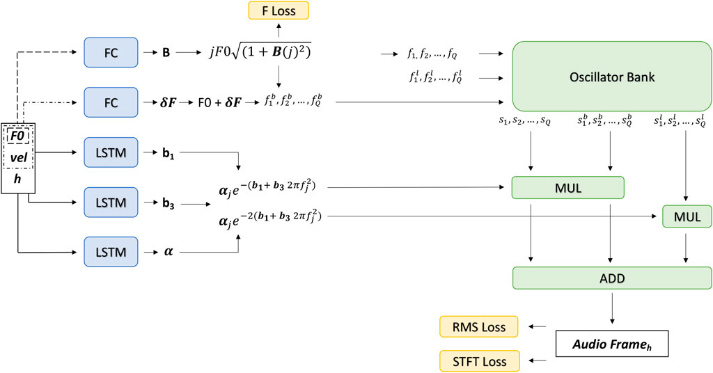
FIGURE 1. Proposed architecture. The model takes as input the key’s fundamental frequency F0 (derived from the MIDI note number), the key velocity vel, and the relative time index h, which represents how long the key has been pressed. F0 is fed to a fully connected network followed by the rectified linear unit activation that computes the inharmonicity factor B. The partial frequencies f1, f2, …, fQ are calculated using Eq. 5 and then are sent to an oscillator bank to generate the sinusoidal signals s1, s2, …, sQ. The key frequency F0, velocity vel, and the index h are the inputs of three LSTM-based networks that predict the values needed to compute exponents and the base for the decay envelope according to Eq. 3. F0 and vel are also the inputs of a fully connected network with tanh activation function that computes the δF, which is the frequency deviation of the main string creating the beating effect. The δF is added to F0 and uses Eq. 5 to calculate the partials’ frequencies
Assuming D as the level of model polyphony, the input will have a dimension of D×3. The F0 values are directed to a fully-connected (FC) ANN, which computes the inharmonicity coefficient B. The value of B varies for each piano note due to differing string lengths and is not time-dependent. In this scenario, an FC network with a single hidden layer with linear activation functions, followed by an output layer with rectified linear unit (ReLU), is adequate to predict B, the value of which can be 0 for certain keys. B is then used to calculate the frequencies fj using Eq. 5. These are fed to the sinusoidal oscillator bank generating the partials.
F0 and vel are inputs of an FC network with no hidden layers and tanh activation function on the output layer. This FC predicts the values representing the δF difference in frequency accounting for the detuning of the sub-strings and creating the beating. Detuning is considered a time-invariant but only key-dependent. The output of the second FC network δF is added to the key’s fundamental frequency F0 and used in Eq. 5 to calculate the frequencies
F0, vel, and h are sent to three parallel LSTM networks to compute the decay envelopes. The first two LSTM networks predict the coefficients b1 and b3 required to compute the decay rate of the key. The last LSTM computes the coefficients αj. We opted for LSTM networks for these three parameters since the model must track time accurately in order to model the percussive envelope of the piano’s sound. The computed decay values are then applied to all sinusoidal signals generated by the oscillator bank. For the phantom partials, the decay rate has a duration that is halved. Finally, the model generates a frame of audio samples by summing all sinusoids related to the key’s frequency, beating, and phantom partials. Continuity of the sinusoidal signals across frames is ensured by an internal audio-rate time index, which is reset at the onset of each note.
4.2 Losses
Three loss functions are used in the training process. The first is the log mean-squared-error (logMSE) loss, utilized in the quasi-harmonic module. The logMSE compares the model’s predicted frequency for the first partial f1 with the target frequency
where δ is used to avoid the zero argument of the logarithm, which in our case is fixed to 1. We use log2 because this is also used in the cent scale, which is the logarithmic unit of measure for musical intervals.
Using the F loss, the model can be anchored to the first partial and helped to match the other partials. The second loss is the mean-squared-error (MSE) of the root-mean-square (RMS) values computed on the whole target and predicted audio frame. This helps the network predict a sequence of audio frames that match the target amplitude envelope. The third is a multi-resolution STFT loss that guides the prediction of the frequency and amplitude envelope of each partial. Both losses are computed on the model’s output sound. The multi-resolution STFT (Engel et al., 2020) loss is defined as in Eq. 7. This loss compares the linear and logarithmic absolute values of STFT with different frequency resolutions using the L1 norm, calculated as the sum of the absolute vector values. We select the window length m to be 512, 1,024, and 2,048.
4.3 Datasets
The dataset used in our experiments includes individual piano notes recorded from a Yamaha Disklavier MX100A, which was controlled via MIDI messages. The piano was tuned using 440 Hz as the reference pitch for the A4 key before the dataset was collected. Sound recording was carried out using a MOTU M41 audio interface connected to an Earthworks M50 measurement microphone2. The microphone was placed inside the piano case a few centimeters away from the instrument strings to minimize the adverse effect of the room acoustic on the recorded data. The interval between each pair of MIDI note-on and note-off messages was fixed to 2 s. This implies that the piano keys were depressed for a duration of 2 s, while each audio recording has a duration of 2.5 s, including 0.5 s after the key release. This duration was sufficient to capture the great majority of the decay’s sound in the selected octaves. Our study focused on the central keyboard range of the piano, considering two octaves of keys from C3 to B4 played at seven different velocities ranging from 60 to 120 with a step of 10. The recording was taken with a sampling rate of 48 kHz and down-sampled to 24 kHz for the training. We choose not to vary the key holding time because this does not affect the natural decay time of the sound nor the parameters influencing the decay rates. Indeed, when the key is released, the string is just damped. Eventually, this feature can be integrated with a separate ADSR block, tuned either manually or with parameters derived by neural modeling.
We computed input vectors starting from the MIDI data, including the key’s fundamental frequency F0, velocity vel, and time index h. Values of F0 are derived from the MIDI note number as
4.4 Experiments and learning
The model is trained using the Adam (Kingma and Ba, 2014) optimizer with gradient norm scaling of 1 (Pascanu et al., 2013) and an initial learning rate of 10–6. Models are trained for 50 epochs. Test losses are computed with the model’s weights that minimize the validation loss throughout the training epochs. With only 168 note-recording examples in total, the dataset is relatively small. These examples encompass seven different velocities for each of the 24 unique keys. We built two training and test sets to evaluate two different scenarios. In the first scenario, the training set includes recordings of all datasets, excluding those related to the key in the middle of the dataset’s range—D4. The recordings of D4 at different velocities are used as the test set. This represents the most challenging case as it evaluates how the model predicts the sound of an unseen key at various velocities. In the second scenario, we train the network using recordings of all keys in the dataset but exclude all middle-velocity examples, which are the recordings at a velocity of 90 for each key used as the test set. Here, the network’s performance is assessed based on its ability to predict the sound produced by seen keys at unseen velocity values. In both scenarios, the validation set consists of 10% of the shuffled training set. Ideally, if aiming at high modeling fidelity, the training should employ a much larger dataset, extended with more velocity and key examples. In practice, we use such a small dataset in two specific testing scenarios to evaluate the ability of our proposed model to interpolate between unseen keys and velocity values. Finally, we also cross-validate the model by repeating the first testing scenario 24 times, each time with a different unseen key, and the second testing scenario 7 times, each with a different unseen velocity value. Models in the cross-validation are trained for 50 epochs.
We have chosen to experiment by sampling the MIDI data at 100 Hz and at 1 kHz, meaning that each MIDI note is broken down in a sequence of samples. We utilize an audio sampling rate of 24 kHz. Thus, each sample drawn from the MIDI data, which we use as model input, aligns with frames of either 240 or 24 audio sample. Therefore, the model’s inference produces frames of 240 or 24 audio samples at a time. This arbitrary choice is a good trade-off between computational complexity and stimulus-to-sound latency. It thus demonstrates the suitability of this modeling technique for low-latency interactive applications, particularly in sound synthesis.
The actual inputs to the model are vectors, each consisting of triplets comprising F0, vel, and h values. Based on the sampling rates specified above, a 2.5-s recording in our dataset corresponds to a sequence of 250 input vectors when dealing with output audio frames that contain 240 samples, and to a sequence of 2,500 input vectors when dealing with output audio frames that contain 24 samples.
The selected number Q of partials is set to 24 because, in the octave region of our dataset, keys usually produce approximately 20–30 partials (Russell and Rossing, 1998). The fully connected layer consists of 32 units, while the LSTM layers present the same number of units as the number of partials. Finally, like Renault et al. (2022), we adopted two stages of learning. First, we tuned the inharmonicity factor using the F loss and, in turn, produced partials as close as possible to the target. Second, we allowed the model to learn the partials’ amplitude envelope using the STFT and RMS losses. During the first phase, only the FC’s weights were trainable, while, in the second, we trained the layers’ weights predicting the decay coefficient b1, b3, αj, and δF. Early experiments showed that this order leads to better accuracy.
5 Results
The first evaluation of the model is based on the test losses obtained in the two test scenarios: in the first, the model predicts the sound of an unseen key during training at different velocities; in the second, the model predicts an unseen velocity for all seen training keys. In the first case, the unseen key is D4 with its associated seven different velocities. In the second case, the unseen velocity is 90. The STFT, F0, and RMS loss values, as defined in Section 4, are reported in Tables 1, 2. F loss values are small for predicted D4 velocities. We computed an approximation of the respective cent deviation (Ellis, 1880), this average also being reported in Table 1 with a max value of 4.46 ⋅ 10–1. Considering that the distance from the previous and next keys is 100 cents, we evaluate the error as perceptually negligible. Table 1 also reports the MSE of the inharmonicity factor B. This is calculated from Eq. 5, with the partial’s index j equal to 1, as follows:
The BMSE values in Table 1 demonstrate that the model effectively predicts the estimated inharmonicity factor B, even for unseen keys. It should be noted that these inharmonicity factors (B,
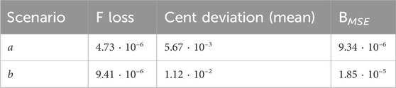
TABLE 1. F loss, cent deviation (mean), and BMSE on the test set across two scenarios: unseen key (a) and unseen velocity (b).
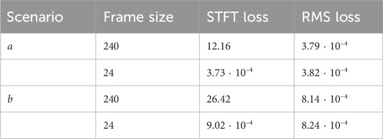
TABLE 2. STFT and RMS losses on the test set for models generating output frames with 240 and 24 audio samples across two scenarios: unseen key (a) and unseen velocity (b).
The absolute value of the STFT loss is smaller in the first scenario, which could be attributed to the relative ease of interpolating between inharmonicity factors of different keys compared to interpolating between the amplitude envelopes at different velocities. Inharmonicity factors typically exhibit nearly linear changes across keys, whereas the energy of partials is subject to more substantial nonlinear variations. However, the absolute value of STFT loss has limited significance in this context because we do not model the noisy component of the piano sound. As a result, the sound generated by the quasi-harmonic module differs perceptually from the actual piano sound. We note that when the model produces only 24 output samples at a time, we observe an even further reduction in STFT loss. Generating fewer samples per iteration is advantageous for the model as it allows for more precise control over the temporal evolution of the partials. A model configured to produce smaller outputs can update its parameters every 1 ms (24 samples), in contrast to every 10 ms (240 samples) for a model that generates larger outputs. Conversely, the RMS loss does not exhibit a notable change in relation to the number of output samples.
To further evaluate the spectral reconstruction capability of the models, we present the spectrograms for both scenarios in Figures 2, 3. Inspection of these figures reveals that the models have successfully learned the temporal unfolding of the partials’ amplitudes without requiring a large neural network. This efficiency is due to the models’ intrinsic understanding of the general shape of the partials’ evolution over time. Despite this, the models exhibit a slight underestimation of the decay time for the higher partials, resulting in a slower decay rate. Moreover, there is a slight underestimation of the amplitudes, which is visible in the logarithmic decibel-scale magnitude spectra with a logarithmic frequency axis (Figures 4, 5). The plots focus on the frequency range [100, 8,000] Hz to better highlight the frequencies of interest, and the FFT frequency resolution set is 2 Hz. In the higher regions of the spectrum, components not yet included in the model, such as noise and other phantom partials, significantly impact the resulting frequency distribution and are expected to cause mismatches. Indeed, the plots compare recorded piano notes with only their predicted harmonic contents. The models accurately predict the first nine partials, while the error increases for higher partials. During experiments, we noted that anchoring f1 with the loss benefits the networks since they then approximate B to align all the partials. However, errors in the inharmonicity factor increase at high frequencies due to the square term in Eq. 5. In the first scenario, the model appears to overestimate the energy in the higher part of the spectrum, while, in the second scenario, it underestimates it, especially for lower notes. The model does not account for all the piano components that affect the sound. It thus lacks the flexibility to accurately emulate the high-frequency part of the spectrum. Consequently, the model exploits the main and phantom partials that it can generate to cover that frequency range, reducing its overall accuracy. On the other hand, the amplitudes are adjusted using LSTMs, which did not completely converge within the 50 training epochs used in our experiments, suggesting that accuracy might improve with additional training epochs.
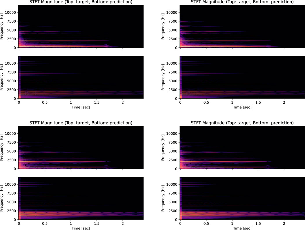
FIGURE 2. Comparison of spectrograms of the model’s output versus the test recordings for key (D4) at velocity values of 60, 80, 100, and 120. The plots compare the recorded notes with the prediction of only their harmonic content. The STFT is computed using windows of 2,048 samples with 75% overlap.
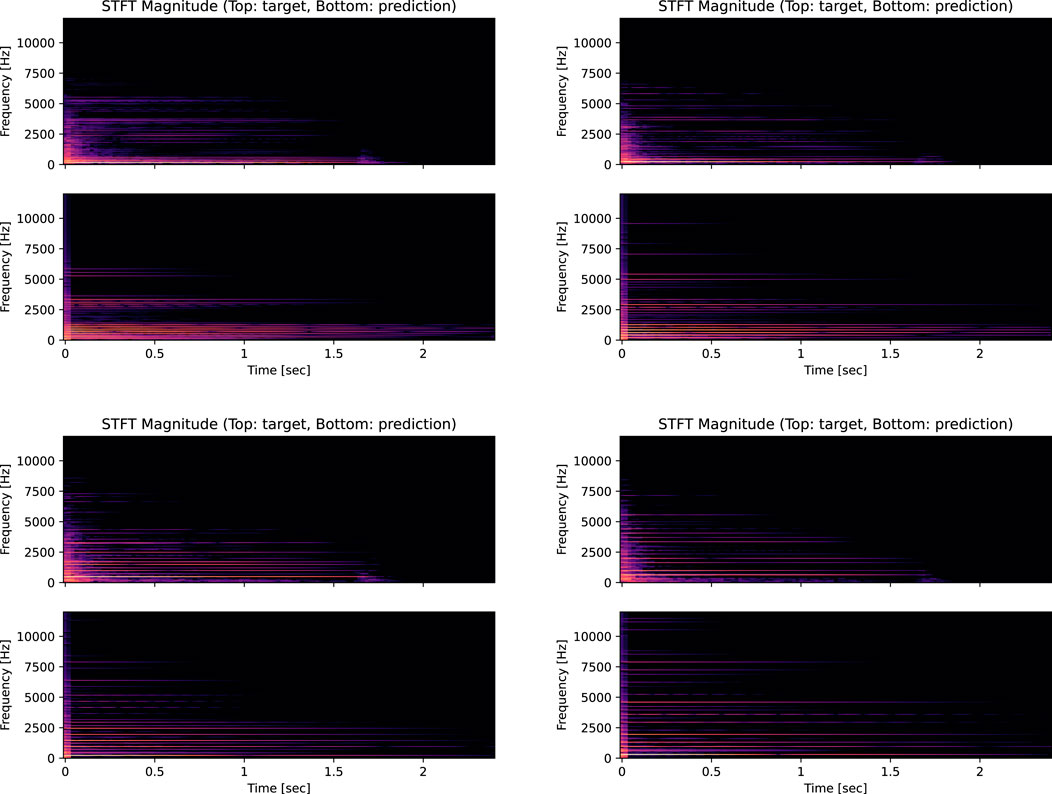
FIGURE 3. Comparison of spectrograms of the model’s output compared versus the test recordings for velocity 90 and keys C3#, G3#, B3, and E4. The plots compare the recorded notes with the prediction of only their harmonic contents. The STFT is computed using windows of 2,048 samples with 75% overlap.
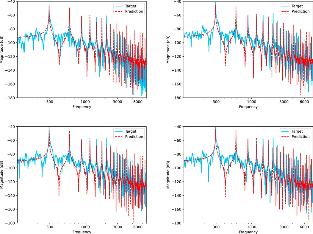
FIGURE 4. Comparison of magnitude spectra of the model’s output versus test recordings for key (D4) at velocity values of 60, 80, 100, and 120. The plots compare the recorded notes (blue) with the prediction (red) of only their harmonic contents. The plots utilize a logarithmic scale on both axes, with frequency limited to the range [100, 8,000] Hz.
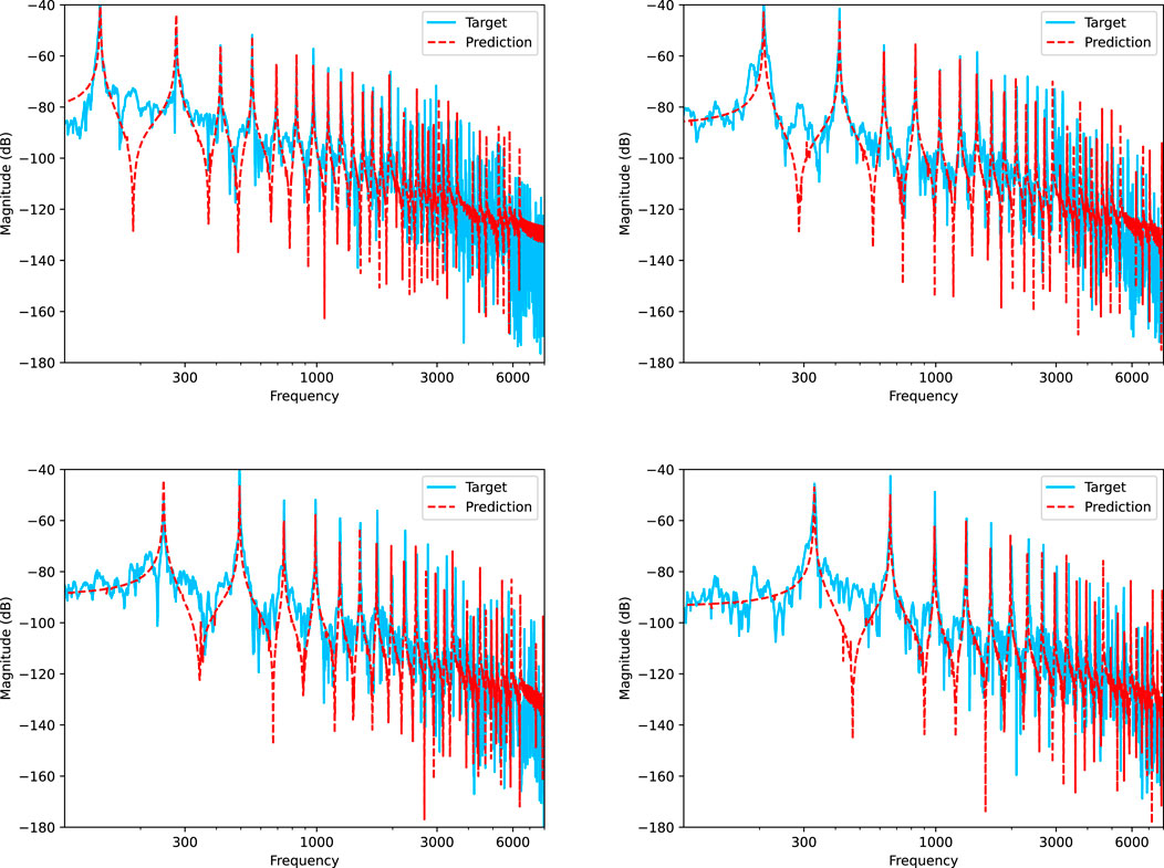
FIGURE 5. Comparison of magnitude spectra of the model’s output versus the test recordings for velocity 90 and keys C3#, G3#, B3, and E4. The plots compare the recorded notes (blue) with the prediction (red) of only their harmonic contents. The plots utilize a logarithmic scale on both axes, with frequency limited to the range [100, 8,000] Hz.
The final feature of the model we evaluated is its ability to simulate the decaying envelopes characteristic of the piano sound. Figure 6 includes plots of the RMS envelopes for the same examples considered in the previous figures across scenarios involving unseen keys and velocities. Generally, the model’s predictions follow the target sound’s decay, characterized by two distinct rates: an initial rapid decline followed by a slower decay rate. However, these two phases are less pronounced in the model’s predictions compared to the actual test notes. Specifically, there is a notable discrepancy in the starting amplitude in the second scenario, which is consistent with the quantitative losses and expectations, considering that the second scenario’s training involved a limited number of velocity examples. Remarkably, with a relatively small training dataset containing only seven different velocity values, the model successfully tracked the decay changes. Additionally, the lack of noise component modeling in the attack phase of the sound contributed to the observed discrepancies.
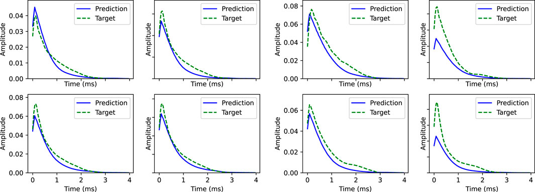
FIGURE 6. Comparison of the RMS of the model’s output versus the test recordings for key (D4) at velocity values of 60, 80, 100, and 120 (left), and for velocity 90 and keys C3#, G3#, B3, and E4 (right). The plots compare the recorded notes (green) with the prediction (blue) of only their harmonic contents. The RMS is computed using windows of 2,400 samples with 75% overlap.
5.1 Cross-validation
Table 3 presents the average STFT loss, RMS loss, and F loss computed on the cross-validation test sets for the unseen key and unseen velocity scenarios. During the cross-validation, keys and velocities at the dataset’s edges were also used as test sets, requiring the model to extrapolate slightly beyond the dataset. The STFT loss values are marginally higher in the unseen key scenario, which differs from the previous evaluation based solely on the D4 test set. Conversely, the trends of RMS and F loss are similar. The unseen key scenario continues to pose greater challenges for RMS accuracy, while the F0 estimates are more precise.
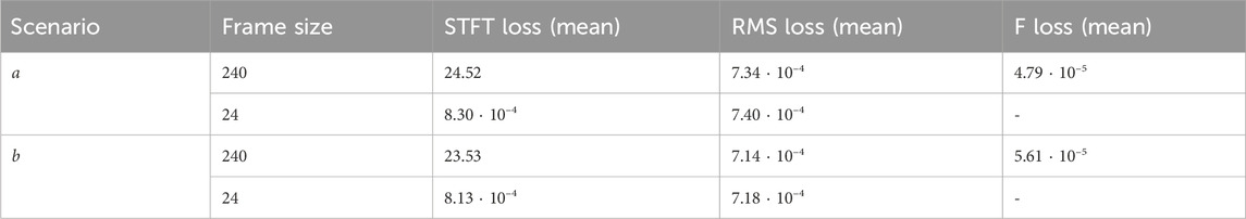
TABLE 3. Mean of the STFT loss, RMS loss, and F loss computed on the test set across the 24 cross-validation trainings in scenario a with unseen keys and across the 7 cross-validation trainings in scenario b with unseen velocities, with models trained for 50 epochs.
Figures 7, 8 illustrate the STFT and RMS losses obtained in the cross-validation, the averages of which are detailed in Table 3. The losses in Figure 7 refer to the model that produces output frames containing 240 audio samples. This figure illustrates losses from the 24 training sessions featuring different unseen keys and resulting from seven training sessions, each with a unique, unseen velocity value. Conversely, Figure 8 presents analogous data but shows losses associated with the model that generates output frames with only 24 audio samples. Although the losses are generally minimal in the unseen key scenario, the trend may not appear uniform at first sight. In particular, predictions for certain keys, especially from D3# to F3#, seem to be less accurate. However, upon inspection of the audio recordings in the dataset, it is evident that the associated signals exhibit higher amplitudes despite having identical MIDI velocities. This is likely due to a loss of calibration in the actuators of the Yamaha Disklavier MX100A used to collect the data, which had been in use for almost 30 years. Amplitude mismatches in the dataset may also arise from other external factors, such as the room’s acoustic response. Nonetheless, the relative error remains comparatively constant when considered in relation to the absolute target amplitude. In the unseen velocity scenario, the STFT and RMS losses consistently increase with the velocity value. On the one hand, the error relative to the target amplitude remains fairly constant, as discussed in the previous scenario. However, larger errors at high velocities are also expected because phenomena such as bridge-string coupling and differing string polarization tend to become more dominant, affecting the resulting sound. Trends remain consistent in both scenarios, regardless of whether the model produces output frames containing 240 or 24 audio samples. Overall, as observed earlier, the model demonstrates better accuracy when working with smaller frames.
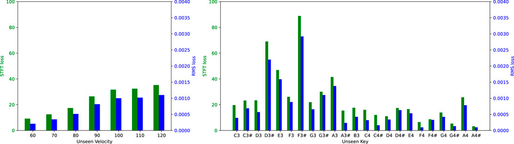
FIGURE 7. STFT loss (green) and RMS loss (blue) for models generating output frames with 240 audio samples, compared across the cross-validation for unseen velocities (left) and unseen keys (right).
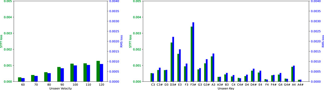
FIGURE 8. STFT loss (green) and RMS loss (blue) for models generating output frames with 24 audio samples, compared across the cross-validation for unseen velocities (left) and unseen keys (right).
5.2 Computational efficiency
Table 4 provides the number of trainable parameters and FLOPs required for model inference. We considered models generating output frames with 24 and 240 audio samples, polyphony levels of 1 and 88, with the latter representing the case of a full-sized piano keyboard. As expected, polyphony has a significant impact on computational complexity, especially when the model produces smaller output frames. On the other hand, the model has lower input-to-sound latency when it produces smaller frames. In our case, when using 24 samples, the architecture has a latency of 1 ms, while, with 240 samples, latency is still reasonable at approximately 10 ms because the time required for the hammer to travel and hit the strings is approximately 7 ms at high speeds. For practical applications, latency values in this range can be acceptable, contributing to reducing the required number of operations per audio sample. Comparing this with similar work, the model in Renault et al. (2022) has 281.5k trainable parameters (excluding those related to the reverb) with a polyphony level of 16. In contrast, our model has only 3,428 trainable parameters at the same level of polyphony. However, we expect our model to grow when modeling the noisy components and the coupling between close keys.
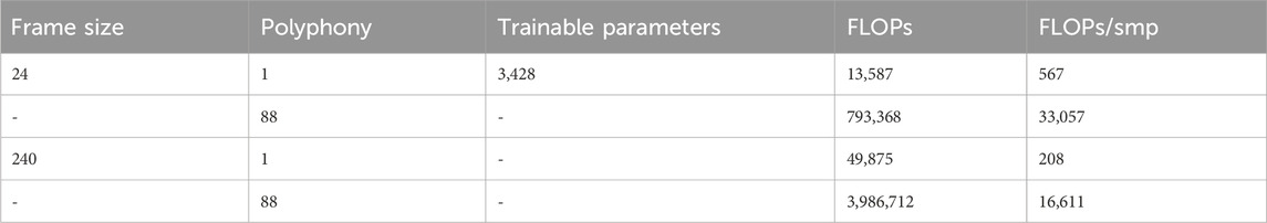
TABLE 4. Number of trainable parameters, FLOPs for audio frame inference, and FLOPs per audio sample for the models with different output frame sizes and polyphony.
6 Discussion
We introduced a method for modeling piano instruments using knowledge of physics and the DDSP framework. The model uses end-to-end learning to tune the parameters, informed by mathematical formulas derived from a comprehensive understanding of the instrument’s physics. We focused on the singular key’s quasi-harmonic content, informing the model with the inharmonicity factor, partials’ decay times, partials’ generation due to longitudinal displacements, and beating. Furthermore, our approach is modular. Therefore, the model is extendable: additional features based on physical knowledge can be introduced and learned from existing, pre-trained models. The results showed that our model can learn complex features in the quasi-harmonic content from the target recordings using small datasets and networks with a small number of trainable parameters. In addition, the model appears to be capable of good generalization, consistently learning from data across different keys and velocities. However, some discrepancies remain in target spectrogram matching, especially prominent in higher frequencies, where the energy decay of partials is harder to track. The discrepancies are primarily attributable to the model’s incompleteness and potential biases in our small dataset. The losses associated with the inharmonicity factor B are contingent upon accurately estimating the frequency of the first partial. Any imprecision in this estimation can significantly impact the generation of the higher partials. Therefore, enhancing the estimation of B could potentially lead to improved performance of the model. Additionally, the piano itself may have defects due to age or mistuning, which pose challenges for inclusion in the model. In future work, we aim to explore alternative methods for estimating B, such as determining its value by fitting a larger set of partials extracted from the dataset with robust tracking algorithms. Additionally, exploring the integration of a more accurate equation for the inharmonicity factor (Fletcher and Rossing, 2012) could potentially improve the high-frequency match.
The proposed approach offers an alternative to physical modeling, preventing the need of solving nonlinear partial differential equations while still taking them into account. It also addresses problems associated with the black-box model of traditional deep learning techniques. Moreover, the DDSP framework allows the design of low-latency architectures with less computational complexity. By integrating principles of physics, the model enhances efficiency and accuracy while minimizing training time. Hybrid modeling methods can bypass challenges related to tracking long and complex temporal structures in the audio signal, which are often encountered when modeling musical devices, and facilitate achieving good performances even when utilizing relatively smaller networks and datasets. Additionally, a decrease in the size of the inference output audio frame does not compromise the model’s accuracy, as evidenced in the results. This modular method embraces flexibility and reusability, as many instruments share similar sound production processes.
The work presented here does not constitute a comprehensive model; hence, the audio generated does not closely emulate the sound of a real acoustic piano. However, when informally listening to the generated sound, the tonality, inharmonicity, and percussive nature of the sound are clearly recognizable. Future work will also include the development of the piano’s noise component. This component, created largely by the initial hammer–string collision and subsequent piano structure vibrations, is crucial for achieving sound fidelity, particularly in the initial audio transient of the piano. While previous methods have used ANNs to predict the filter for a noise source, integrating knowledge of physics in modeling the hammer–string collision could yield beneficial results.
Another aspect to integrate into our work is the damping that affects string vibrations when the key is released. This damping could be separately modeled with an ADSR block, which can be designed using classic DSP algorithms or exploiting machine learning techniques. While we considered the double-frequency effect due to longitudinal displacements, other partials generated by the combined effect of sum and difference of the modes, bearing in mind transverse waves, should also be included, allowing the model to generate these additional sinusoids. Finally, the model must consider more complex scenarios such as simultaneous note playing, which would involve modeling the interaction between different keys via the bridge where vibrations of strings can influence the generation of modes in strings belonging to other keys.
The audio examples, dataset, source code, and trained models described in this paper are available online3.
Data availability statement
The datasets presented in this study can be found in online repositories. The names of the repository/repositories and accession number(s) can be found at https://www.kaggle.com/datasets/riccardosimionato/pianorecordingssinglenotes.
Author contributions
RS: data curation, investigation, methodology, and writing–original draft. SF: writing–review and editing. SH: writing–review and editing.
Funding
The author(s) declare that no financial support was received for the research, authorship, and/or publication of this article.
Conflict of interest
The authors declare that the research was conducted in the absence of any commercial or financial relationships that could be construed as a potential conflict of interest.
Publisher’s note
All claims expressed in this article are solely those of the authors and do not necessarily represent those of their affiliated organizations, or those of the publisher, the editors, and the reviewers. Any product that may be evaluated in this article, or claim that may be made by its manufacturer, is not guaranteed or endorsed by the publisher.
Footnotes
1https://motu.com/en-us/products/m-series/m4/
2https://earthworksaudio.com/measurement-microphones/m30/
3https://github.com/RiccardoVib/Physics-Informed-Differentiable-Piano
References
Adrien, J. M., Causse, R., and Ducasse, E. (1988). “Sound synthesis by physical models, application to strings,” in Audio engineering society convention (Paris, France: Audio Engineering Society), 84.
Aouameur, C., Esling, P., and Hadjeres, G. (2019). Neural drum machine: an interactive system for real-time synthesis of drum sounds. arXiv preprint arXiv:1907.02637.
Askenfelt, A., and Jansson, E. V. (1991). From touch to string vibrations. ii: the motion of the key and hammer. J. Acoust. Soc. Am. 90, 2383–2393. doi:10.1121/1.402043
Bank, B. (2009). “Energy-based synthesis of tension modulation in strings,” in Proceedings of the 12th International Conference on Digital Audio Effects (DAFx-09), 365–372.
Bank, B., and Sujbert, L. (2005). Generation of longitudinal vibrations in piano strings: from physics to sound synthesis. J. Acoust. Soc. Am. 117, 2268–2278. doi:10.1121/1.1868212
Bengio, S., Vinyals, O., Jaitly, N., and Shazeer, N. (2015). Scheduled sampling for sequence prediction with recurrent neural networks. Adv. neural Inf. Process. Syst. 28. doi:10.5555/2969239.2969370
Bentsen, L. Ø., Simionato, R., Benedikte, B. W., and Krzyzaniak, M. J. (2022). “Transformer and lstm models for automatic counterpoint generation using raw audio,” in Proceedings of the Sound and Music Computing Conference (Society for Sound and Music Computing).
Bilbao, S., Ducceschi, M., and Webb, C. J. (2019). “Large-scale real-time modular physical modeling sound synthesis,” in Proceedings of the 22nd Conference of Digital Audio Effects (DAFx-19), 1–8.
Bitton, A., Esling, P., Caillon, A., and Fouilleul, M. (2019). Assisted sound sample generation with musical conditioning in adversarial auto-encoders. arXiv preprint arXiv:1904.06215.
Brunton, S. L., Noack, B. R., and Koumoutsakos, P. (2020). Machine learning for fluid mechanics. Annu. Rev. fluid Mech. 52, 477–508. doi:10.1146/annurev-fluid-010719-060214
Cai, S., Mao, Z., Wang, Z., Yin, M., and Karniadakis, G. E. (2021). Physics-informed neural networks (pinns) for fluid mechanics: a review. Acta Mech. Sin. 37, 1727–1738. doi:10.1007/s10409-021-01148-1
Carrier, G. F. (1945). On the non-linear vibration problem of the elastic string. Q. Appl. Math. 3, 157–165. doi:10.1090/qam/12351
Chabassier, J., Chaigne, A., and Joly, P. (2013). Modeling and simulation of a grand piano. J. Acoust. Soc. Am. 134, 648–665. doi:10.1121/1.4809649
Chabassier, J., Chaigne, A., and Joly, P. (2014). Time domain simulation of a piano. part 1: model description. ESAIM Math. Model. Numer. Analysis 48, 1241–1278. doi:10.1051/m2an/2013136
Chaigne, A., and Askenfelt, A. (1994). Numerical simulations of piano strings. i. a physical model for a struck string using finite difference methods. J. Acoust. Soc. Am. 95, 1112–1118. doi:10.1121/1.408459
Chen, J., Tan, X., Luan, J., Qin, T., and Liu, T. (2020). Hifisinger: towards high-fidelity neural singing voice synthesis. arXiv preprint arXiv:2009.01776.
Chen, R. T. Q., Rubanova, Y., Bettencourt, J., and Duvenaud, D. K. (2018). Neural ordinary differential equations. Adv. neural Inf. Process. Syst. 31. doi:10.5555/3327757.3327764
Child, R., Gray, S., Radford, A., and Sutskever, I. (2019). Generating long sequences with sparse transformers. arXiv preprint arXiv:1904.10509.
Conklin, J., and Harold, A. (1996). Design and tone in the mechanoacoustic piano. part i. piano hammers and tonal effects. J. Acoust. Soc. Am. 99, 3286–3296. doi:10.1121/1.414947
Cooper, E., Wang, X., and Yamagishi, J. (2021). Text-to-speech synthesis techniques for midi-to-audio synthesis. arXiv preprint arXiv:2104.12292.
Défossez, A., Zeghidour, N., Usunier, N., Bottou, L., and Bach, F. (2018). Sing: symbol-to-instrument neural generator. Adv. neural Inf. Process. Syst. 31. doi:10.5555/3327546.3327579
Desai, S. A., Mattheakis, M., Sondak, D., Protopapas, P. D., and Roberts, S. J. (2021). Port-Hamiltonian neural networks for learning explicit time-dependent dynamical systems. Phys. Rev. E 104, 034312. doi:10.1103/physreve.104.034312
Dieleman, S., and Schrauwen, B. (2014). “End-to-end learning for music audio,” in Proceedings of the IEEE International Conference on Acoustics, Speech and Signal Processing (ICASSP) (IEEE), 6964–6968.
Donahue, C., McAuley, J., and Puckette, M. (2018). Adversarial audio synthesis. arXiv preprint arXiv:1802.04208.
Dong, H., Zhou, C., Berg-Kirkpatrick, T., and McAuley, J. (2022). “Deep performer: score-to-audio music performance synthesis,” in Proceedings of the IEEE International Conference on Acoustics, Speech and Signal Processing (ICASSP) (IEEE), 951–955.
Drioli, C., and Rocchesso, D. (1998). “Learning pseudo-physical models for sound synthesis and transformation,” in SMC’98 Conference Proceedings. 1998 IEEE International Conference on Systems, Man, and Cybernetics (Cat. No. 98CH36218) (IEEE), 1085–1090.
Drysdale, J., Tomczak, M., and Hockman, J. (2020). “Adversarial synthesis of drum sounds,” in Proceedings of the International Conference on Digital Audio Effects (DAFx).
Engel, J., Agrawal, K. K., Chen, G. I. S., Donahue, C., and Roberts, A. (2019). Gansynth: adversarial neural audio synthesis. arXiv preprint arXiv:1902.08710.
Engel, J., Hantrakul, L., Gu, C., and Roberts, A. (2020). Ddsp: differentiable digital signal processing. arXiv preprint arXiv:2001.04643.
Engel, J., Resnick, C., Roberts, A., Dieleman, S., Norouzi, M., Eck, D., et al. (2017a). “Neural audio synthesis of musical notes with wavenet autoencoders,” in Proceedings of the International Conference on Machine Learning (Sydney, Australia: PMLR), 1068–1077.
Etchenique, N., Collin, S. R., and Moore, T. R. (2015). Coupling of transverse and longitudinal waves in piano strings. J. Acoust. Soc. Am. 137, 1766–1771. doi:10.1121/1.4916708
Fletcher, N. H., and Rossing, T. D. (2012). The physics of musical instruments. Springer Science & Business Media.
Gabrielli, L., Tomassetti, S., Squartini, S., and Zinato, C. (2017). “Introducing deep machine learning for parameter estimation in physical modelling,” in Proceedings of the 20th international conference on digital audio effects.
Gabrielli, L., Tomassetti, S., Zinato, C., and Piazza, F. (2018). End-to-end learning for physics-based acoustic modeling. IEEE Trans. Emerg. Top. Comput. Intell. 2, 160–170. doi:10.1109/tetci.2017.2787125
Giordano, N., and Winans, J. P. (2000). Piano hammers and their force compression characteristics: does a power law make sense? J. Acoust. Soc. Am. 107, 2248–2255. doi:10.1121/1.428505
Goodfellow, I., Pouget-Abadie, J., Mirza, M., Xu, B., Warde-Farley, D., Ozair, S., et al. (2014). Generative adversarial nets. Proc. Adv. neural Inf. Process. Syst. 27. doi:10.1145/3422622
Hall, D. E. (1987). Piano string excitation ii: general solution for a hard narrow hammer. J. Acoust. Soc. Am. 81, 535–546. doi:10.1121/1.394919
Hantrakul, L., Engel, J. H., Roberts, A., and Gu, C. (2019). “Fast and flexible neural audio synthesis,” in Ismir.
Hawthorne, C., Stasyuk, A., Roberts, A., Simon, I., Huang, C. A., Dieleman, S., et al. (2018). Enabling factorized piano music modeling and generation with the maestro dataset. arXiv preprint arXiv:1810.12247.
Hinrichsen, H. (2012). Entropy-based tuning of musical instruments. Rev. Bras. Ensino Física 34, 1–8. doi:10.1590/s1806-11172012000200004
Ho, J., Jain, A., and Abbeel, P. (2020). Denoising diffusion probabilistic models. Adv. Neural Inf. Process. Syst. 33, 6840–6851. doi:10.5555/3495724.3496298
Hono, Y., Hashimoto, K., Oura, K., Nankaku, Y., and Tokuda, K. (2021). Sinsy: a deep neural network-based singing voice synthesis system. Proc. IEEE/ACM Trans. Audio, Speech, Lang. Process. 29, 2803–2815. doi:10.1109/taslp.2021.3104165
Kalchbrenner, N., Elsen, E., Simonyan, K., Noury, S., Casagrande, N., Lockhart, E., et al. (2018). “Efficient neural audio synthesis,” in Proceedings of the International Conference on Machine Learning (Stockholm, Sweden: PMLR), 2410–2419.
Kim, J. W., Bittner, R., Kumar, A., and Bello, J. P. (2019). “Neural music synthesis for flexible timbre control,” in Proceedings of the IEEE International Conference on Acoustics, Speech and Signal Processing (ICASSP) (IEEE), 176–180.
Kim, S., Lee, S., Song, J., Kim, J., and Yoon, S. (2018). Flowavenet: a generative flow for raw audio. arXiv preprint arXiv:1811.02155.
Kingma, D. P., and Ba, J. (2014). Adam: a method for stochastic optimization. Int. Conf. Learn. Represent.
Kong, Z., Ping, W., Huang, J., Zhao, K., and Catanzaro, B. (2020). Diffwave: a versatile diffusion model for audio synthesis. arXiv preprint arXiv:2009.09761.
Kuznetsov, B., Parker, J. D., and Esqueda, F. (2020). Differentiable iir filters for machine learning applications. Proc. Int. Conf. Digital Audio Eff., 297–303.
Lavault, A., Roebel, A., and Voiry, M. (2022). Stylewavegan: style-based synthesis of drum sounds with extensive controls using generative adversarial networks. arXiv preprint arXiv:2204.00907.
Legge, K., and Fletcher, N. H. (1984). Nonlinear generation of missing modes on a vibrating string. J. Acoust. Soc. Am. 76, 5–12. doi:10.1121/1.391007
Li, N., Liu, S., Liu, Y., Zhao, S., and Liu, M. (2019). Neural speech synthesis with transformer network. Proc. AAAI Conf. Artif. Intell. 33, 6706–6713. doi:10.1609/aaai.v33i01.33016706
Liu, J., Li, C., Ren, Y., Chen, F., and Zhao, Z. (2022). Diffsinger: singing voice synthesis via shallow diffusion mechanism. Proc. AAAI Conf. Artif. Intell. 36, 11020–11028. doi:10.1609/aaai.v36i10.21350
Lu, P., Wu, J., Luan, J., Tan, X., and Zhou, L. (2020). Xiaoicesing: a high-quality and integrated singing voice synthesis system. arXiv preprint arXiv:2006.06261.
Mauch, M., and Dixon, S. (2014). “pyin: a fundamental frequency estimator using probabilistic threshold distributions,” in 2014 ieee international conference on acoustics, speech and signal processing (icassp) (IEEE), 659–663.
Mehri, S., Kumar, K., Gulrajani, I., Kumar, R., Jain, S., Sotelo, J., et al. (2016). Samplernn: an unconditional end-to-end neural audio generation model. arXiv preprint arXiv:1612.07837
Morise, M., Yokomori, F., and Ozawa, J. (2016). World: a vocoder-based high-quality speech synthesis system for real-time applications. IEICE Trans. Inf. Syst. 99, 1877–1884. doi:10.1587/transinf.2015edp7457
Moseley, B., Markham, A., and Nissen-Meyer, T. (2020a). Solving the wave equation with physics-informed deep learning. arXiv preprint arXiv:2006.11894.
Moseley, B., Nissen-Meyer, T., and Markham, A. (2020b). Deep learning for fast simulation of seismic waves in complex media. Solid earth. 11, 1527–1549. doi:10.5194/se-11-1527-2020
Nistal, J., Lattner, S., and Richard, G. (2020). Drumgan: synthesis of drum sounds with timbral feature conditioning using generative adversarial networks. arXiv preprint arXiv:2008.12073.
Oord, A., Li, Y., Babuschkin, I., Simonyan, K., Vinyals, O., Kavukcuoglu, K., et al. (2018). “Parallel wavenet: fast high-fidelity speech synthesis,” in Proceedings of the International conference on machine learning (Stockholm, Sweden: PMLR), 3918–3926.
Paganini, M., de Oliveira, L., and Nachman, B. (2018). Accelerating science with generative adversarial networks: an application to 3d particle showers in multilayer calorimeters. Phys. Rev. Lett. 120, 042003. doi:10.1103/physrevlett.120.042003
Parker, J. D., Schlecht, S. J., Rabenstein, R., and Schäfer, M. (2022). Physical modeling using recurrent neural networks with fast convolutional layers. arXiv preprint arXiv:2204.10125.
Pascanu, R., Mikolov, T., and Bengio, Y. (2013). “On the difficulty of training recurrent neural networks,” in Int. Conf. on machine learning (Atlanta, GA, United States: Pmlr), 1310–1318.
Ping, W., Peng, K., Gibiansky, A., Arik, S. O., Kannan, A., Narang, S., et al. (2018). “Deep voice 3: 2000-speaker neural text-to-speech,” in Proceedings of the International Conference on Learning Representations, 214–217.
Ping, W., Peng, K., Zhao, K., and Song, Z. (2020). “Waveflow: a compact flow-based model for raw audio,” in Proceedings of the International Conference on Machine Learning (PMLR), 7706–7716.
Podlesak, M., and Lee, A. R. (1988). Dispersion of waves in piano strings. J. Acoust. Soc. Am. 83, 305–317. doi:10.1121/1.396432
Prenger, R., Valle, R., and Catanzaro, B. (2019). “Waveglow: a flow-based generative network for speech synthesis,” in Proceedings of the IEEE International Conference on Acoustics, Speech and Signal Processing (ICASSP) (IEEE), 3617–3621.
Raissi, M., Perdikaris, P., and Karniadakis, G. E. (2017). Physics informed deep learning (part i): data-driven solutions of nonlinear partial differential equations. arXiv preprint arXiv:1711.10561.
Ramires, A., Chandna, P., Favory, X., Gómez, E., and Serra, X. (2020). “Neural percussive synthesis parameterised by high-level timbral features,” in Proceedings of the IEEE International Conference on Acoustics, Speech and Signal Processing (ICASSP) (IEEE), 786–790.
Rasp, S., Pritchard, M. S., and Gentine, P. (2018). Deep learning to represent subgrid processes in climate models. Proc. Natl. Acad. Sci. 115, 9684–9689. doi:10.1073/pnas.1810286115
Renault, L., Mignot, R., and Roebel, A. (2022). “Differentiable piano model for midi-to-audio performance synthesis,” in Proceedings of the Conference on Digital Audio Effects (DAFx).
Rezende, D., and Mohamed, S. (2015). “Variational inference with normalizing flows,” in Proceedings of the International conference on machine learning (Lille, France: PMLR), 1530–1538.
Rigaud, F., David, B., and Daudet, L. (2011). “A parametric model of piano tuning,” in Proc. of the 14th Int. Conf. on Digital Audio Effects (DAFx-11), 393–399.
Ronneberger, O., Fischer, P., and Brox, T. (2015). “U-net: convolutional networks for biomedical image segmentation,” in Proceedings of the Medical Image Computing and Computer-Assisted Intervention (MICCAI) (Springer), 234–241.
Russell, D., and Rossing, T. (1998). Testing the nonlinearity of piano hammers using residual shock spectra. Acta Acustica United Acustica 84, 967–975. See also https://www.acs.psu.edu/drussell/hammers.html.
Shen, J., Pang, R., Weiss, R. J., Schuster, M., Jaitly, N., Yang, Z., et al. (2018). “Natural tts synthesis by conditioning wavenet on mel spectrogram predictions,” in Proceedings of the International conference on acoustics, speech and signal processing (ICASSP) (IEEE), 4779–4783.
Smith, J. O. (1996). Physical modeling synthesis update. Comput. Music J. 20, 44–56. doi:10.2307/3681331
Smith, J. O. (1991). “Viewpoints on the history of digital synthesis,” in Proceedings of the International Computer Music Conference (Montreal, Canada: INTERNATIONAL COMPUTER MUSIC ACCOCIATION), 1.
Stulov, A. (1995). Hysteretic model of the grand piano hammer felt. J. Acoust. Soc. Am. 97, 2577–2585. doi:10.1121/1.411912
Suzuki, H. (1987). Vibration analysis of a hammer-shank system, J. Acoust. Soc. Am. 81, S83. doi:10.1121/1.2024431
Suzuki, H., and Nakamura, I. (1990). Acoustics of pianos. Appl. Acoust. 30, 147–205. doi:10.1016/0003-682x(90)90043-t
Tan, H. H., Luo, Y., and Herremans, D. (2020). Generative modelling for controllable audio synthesis of expressive piano performance. arXiv preprint arXiv:2006.09833.
Tolstikhin, I., Bousquet, O., Gelly, S., and Schoelkopf, B. (2018). “Wasserstein auto-encoders,” in Sixth International Conference on Learning Representations ICLR 2018.
Välimäki, V., Huopaniemi, J., Karjalainen, M., and Jánosy, Z. (1995). “Physical modeling of plucked string instruments with application to real-time sound synthesis,” in Audio engineering society convention (Paris, France: Audio Engineering Society), 98.
Vaswani, A., Shazeer, N., Parmar, N., Uszkoreit, J., Jones, L., Gomez, A. N., et al. (2017). “Attention is all you need,” in Proceedings of the Advances in neural information processing systems, 5998–6008.
Verma, P., and Chafe, C. (2021). A generative model for raw audio using transformer architectures, 230–237.
Wang, X., Takaki, S., and Yamagishi, J. (2019). “Neural source-filter-based waveform model for statistical parametric speech synthesis,” in Proceedings of the IEEE International Conference on Acoustics, Speech and Signal Processing (ICASSP) (IEEE), 5916–5920.
Weinreich, G. (1977). Coupled piano strings. J. Acoust. Soc. Am. 62, 1474–1484. doi:10.1121/1.381677
Wilkinson, W. (2019). Gaussian process modelling for audio signals. Ph.D. thesis. Queen Mary University of London.
Wu, D.-Y., Hsiao, W.-Y., Yang, F.-R., Friedman, O., Jackson, W., Bruzenak, S., et al. (2022). Ddsp-based singing vocoders: a new subtractive-based synthesizer and a comprehensive evaluation. Proc. ISMIR 2022.
Yanagisawa, T., and Nakamura, K. (1982). “Dynamic compression characteristics of piano hammer,” in Transactions of musical acoustics technical group meeting of the acoustic society of Japan, 1.
Yanagisawa, T., Nakamura, K., and Aiko, H. (1981). Experimental study on force-time curve during the contact between hammer and piano string. J. Acoust. Soc. Jpn. 37, 627–633.
Yuki, O., Keisuke, I., Shinnosuke, T., Ryosuke, Y., Takahiro, F., and Yoichi, Y. (2020). Onomatopoeia.
Keywords: spectral modeling, physics-informed modeling, acoustic modeling, machine learning, piano synthesis, differentiable digital signal processing
Citation: Simionato R, Fasciani S and Holm S (2024) Physics-informed differentiable method for piano modeling. Front. Sig. Proc. 3:1276748. doi: 10.3389/frsip.2023.1276748
Received: 12 August 2023; Accepted: 28 December 2023;
Published: 13 February 2024.
Edited by:
Cumhur Erkut, Aalborg University, DenmarkReviewed by:
Alberto Bernardini, Polytechnic University of Milan, ItalyRémi Mignot, Institut de Recherche et Coordination Acoustique Musique (IRCAM), France
Copyright © 2024 Simionato, Fasciani and Holm. This is an open-access article distributed under the terms of the Creative Commons Attribution License (CC BY). The use, distribution or reproduction in other forums is permitted, provided the original author(s) and the copyright owner(s) are credited and that the original publication in this journal is cited, in accordance with accepted academic practice. No use, distribution or reproduction is permitted which does not comply with these terms.
*Correspondence: Riccardo Simionato, cmljY2FyZG8uc2ltaW9uYXRvQGltdi51aW8ubm8=