 Danilo Orlando1*
 Alfonso Farina2
- 1University Niccolò Cusano, Rome, Italy
- 2Consultant, Rome, Italy
In this letter, we address the problem of phase-only transmit beamforming to generate a wide beam with an almost flat mainlobe for phased arrays. Instead of resorting to time-demanding optimization procedures, the proposed method is grounded on the Fourier analysis and exploits the fact that radiation pattern can be written as the Fourier transform of the aperture illumination function. In this context, we consider a complex linear frequency modulated illumination function and derive the equations allowing for a control of the beam width. The related computational complexity is linear in the number of the array elements. The numerical examples show the effectiveness of the proposed method in forcing the desired beam shape with good sidelobes’ properties and also in comparison with an iterative competitor.
1 Introduction
Nowadays, modern radars are equipped with phased arrays whose flexibility allow for the development of the multifunction systems where the search and track functions (as well as other advanced functions) coexist without interfering with each other. This capability is strongly related to the beam agility provided by electronic scanning (Melvin, 2012) or, equivalently, electronic beamforming. The advances in technology and digitalization have made it possible to conceive “fully-digital” system architectures with high computational throughput. In this context, Digital BeamForming (DBF) techniques take advantage of the aforementioned technological benefits by combining digital samples at the output of each channel to shape the resulting array beam pattern according to specific requirements and/or the radar function under operation.
Focusing on the search function, the objective of the system consists in scanning the search volume of interest subject to requirements related to reaction time, transmitted energy, priority level assigned to other functions by the system scheduler, and number of decisions in the unit time interval (Melvin and Scheer, 2013). Therefore, for long-range radars, the transmitted energy should ensure that the echoes (also including the losses associated with the channels) of a target located at the maximum distance specified by the system requirements is sufficient to achieve the required probability of detection. For this reason, it would be appropriate to use the transmitter amplifiers in their saturation region, namely to transmit the maximum available power. In such a situation, the number of degrees of freedom for DBF on transmit decreases since the amplitudes of the weights applied to each antenna element are constrained to be constant. As a consequence, DBF on transmit can be accomplished by only exploiting the phase values of the complex weights. In addition, time requirements, the size of the solid angle over which the search is conducted, and the number of range bins within the radar window might limit the scan strategy due to the number of decisions per unit time. In this case, it would be suitable to cover the angular region under surveillance with a low number of pointing directions. To this end, the mainbeam should be sufficiently wide and with a limited ripple in order to ensure a coverage that is as uniform as possible along the azimuth and/or the elevation dimensions.
Most of phase-only (or constant modulus) beamforming techniques are grounded on iterative/numerical optimization procedures. In fact, the constant modulus constraint makes the problem nonconvex and NP-hard (Cong et al., 2022). To solve it, some solutions are obtained through a semidefinite relaxation of the constraint to transform the optimization problem into a convex problem that can be solved by means of well-known numerical tools [(Gershman et al., 2010; Tranter et al., 2016; Tranter et al., 2017; Rixon Fuchs et al., 2022), and references therein]. Other existing strategies exploit statistical and evolutionary methods to find solutions as close as possible to the optimal one (Hatam, 2022). Suitable combinations of the aforementioned approaches can also be found in (Hatam, 2022). Besides the goodness of the proposed solutions in terms of optimality, reducing the computational requirements represents another critical aspect related to the design of beamforming methods. This fact is corroborated by the effort of the scientific community aimed at devising fast iterative/numerical beamforming algorithms (Farina, 1992; Kautz, 1999; Sun and Li, 2003; Demir and Tuncer, 2014; Webster et al., 2015; Tranter et al., 2016; Alhujaili et al., 2019; Liu et al., 2020; Pallotta et al., 2021; Zhang et al., 2021; Angeletti et al., 2022; Cong et al., 2022).
In this letter, we describe a phase-only transmit beamforming method for phased array that does not rely on any iterative/numerical optimization routine. It allows us to generate “an almost” flat beam whose width in terms of angular coverage can be easily set without running any numerical procedure when the radar changes its pointing direction. To this end, we exploit an elementary property of antenna theory, namely that in the far field, the variation of the electronic field intensity can be written as the (spatial) Fourier transform of the aperture illumination function. In the case of phased arrays, the radiation pattern can be obtained from the Discrete Fourier Transform (DFT) of the weights applied to each array element (Skolnik, 2001; Richards, 2014). Therefore, we reason in terms of the Fourier analysis and we find a sequence of phasors with constant modulus whose power spectral density satisfies the system requirements in terms of desired beam width and flatness. Such an approach is new and appears here for the first time (at least to the best of authors’ knowledge). Recalling that the Fourier transform of a complex Linear Frequency Modulated (LFM) pulse can be approximated by a rectangular window with a duration equal to the signal bandwidth (see the stationary phase method) (Papoulis, 1977), a sequence of weights can be drawn from such a signal. Thus, we establish the analytical link between the spatial bandwidth and the angular coverage of interest along the azimuth and elevation directions also verifying the condition that avoids grating lobes. The final weights can be obtained through the Hadamard product between the steering vector at a given pointing direction and these coefficients, hence requiring a number of operations that is linear in the number of array elements and allows for real-time and fast implementation. The numerical examples are obtained by using synthetic data and comparing the proposed approach with a suitable iterative competitor. The results show the superiority of the proposed approach over the considered iterative competitor in terms of computational requirements as well as desired response. Specifically, the variation of the beam width can be accomplished in a straightforward manner without any iterative and time-demanding procedure. Moreover, the mainbeam experiences limited ripples also in the presence of quantized phasors.
The remainder of this letter is organized as follows. The next section describes the proposed method and provides the link between the angular sector to be covered and the spatial frequency bandwidth. Section 3 contains numerical examples obtained with synthetic data. Finally, concluding remarks and possible future research tracks are outlined in Section 4.
2 Method description
In this section, we derive a procedure that allows the system engineer to compute the weights of the beamformer assuming that the system is equipped with equally spaced elements arrayed in a rectangular grid as depicted in Figure 1 where the array is looking towards the z-axis.1 Now, notice that given the Fourier transform of a finite-duration analog signal, it is possible to express the DFT of a sequence extracted from the analog signal as a function of the original spectrum. In fact, the Discrete Time Fourier Transform (DTFT) of the finite-duration sequence is a periodic extension with a step equal to the sampling frequency of the analog signal spectrum, whereas the DFT is obtained by sampling the DTFT within the fundamental period (Oppenheim and Schafer, 1975). Thus, for simplicity, we proceed by considering a rectangular continuous aperture (see also Figure 1) and observe that the two-dimensional field-intensity pattern is given by (Stutzman and Thiele, 2012)
where a(x, y) is the 2-dimensional aperture illumination function that accounts for the finite aperture size along the x-axis, Dx say, and the finite aperture size along the y-axis, Dy say, i.e.,
with f(x, y) a generic function and
λ is the carrier wavelength, while θ and ϕ are defined in Figure 1. Let us introduce the direction cosines u = sin θ cos ϕ and v = sin θ sin ϕ (Mailloux, 2018), then (1) can be recast as
where A ∝ B means that A is proportional to B, α0 = x/λ, and β0 = y/λ. Notice that the last equation represents the 2-dimensional Fourier transform of the illumination function. Therefore, according to the spectral properties of such a function, different beam shapes can be obtained.
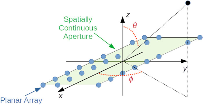
FIGURE 1. Geometry of the antenna array.
As stated in Section 1, we are interested in synthesizing a radiation pattern by exploiting the phase information only and that exhibits a tunable width along both azimuth and elevation. To this end, we set
that is a 2-dimensional LFM where Kh = Bh/Dh, h ∈ {x, y}, is the so-called chirp rate along the h-axis and Bh > 0 the corresponding spatial bandwidth. Replacing (5) in (4), we obtain
where
where Cx > 0 and Cy > 0 are suitable constants. As a consequence, the spatial frequency components are nonnegligible when the following inequalities hold
Let us denote by φ and ϑ the azimuth and elevation angles, respectively, and observe that (Richards, 2014; Mailloux, 2018)
Thus, from (9) and 10, we can write
and denoting by ϑ0 ∈ [0, π/2] the value of ϑ such that the equality holds, we obtain
Now, given ϑ0 ∈ [0, π/2], using (8) and 10, we come up with the following inequality
Let φ0 ∈ [0, π/2] be a value for the azimuth angle such that the equality is true, then, we can write
It follows that Bx and By can be set as
where φ0 and ϑ0 allow for the control of the beam width along the azimuth and elevation dimensions.
Finally, it is important to underline that if the inter-element distances Δx and Δy between two adjacent elements along x and y axes, respectively, are such that
Gathering the above results, the illumination function has the following form
and the corresponding weight vector for the planar rectangular array is obtained by sampling a(x, y) at the spatial sampling frequency associated with the array. Assuming that the sampling space is λ/2, the corresponding weights are
where recall that φ0 and ϑ0 control the beam aperture, (⋅)T stands for transpose,
Nx is the number of elements along the x-axis, Ny is the number of elements along the y-axis, ⊙ is the Hadamard product, and, given
3 Illustrative examples and discussion
In this section, we provide some numerical examples to highlight pros. and cons. of the proposed beamforming strategy. For comparison purposes, we also plot the results obtained by means of the simple Gradient Projection Algorithm (GPA) proposed in (Tranter et al., 2017) since it is light from a computational point of view and allows us to set some constraints to suitably shape the final beam. Specifically, such an algorithm is used to solve the following problem
where
It is clear that GPA is more time-demanding than the proposed strategy whose advantages in terms of required operations are quite evident. In fact, as highlighted at the end of the previous section, the weight vector w is set once and for all and then is multiplied by the array manifold at a given direction. On the other hand,
Let us start by investigating the nominal behavior of the proposed strategy over synthetic data and considering a uniformly spaced rectangular array with Nx = 65, Ny = 65, and inter-element spacing λ/2 (notice that in this case the array manifold as well as the beamforming weights are functionally independent of λ).
In Figures 2, 3, we show the radiation patterns of the proposed approach and GPA assuming a two-side aperture of about 10° (i.e., φ0 = ϑ0 = 5°) and a pointing direction equal to 0° in azimuth and elevation. It turns out that both algorithms allow for a control of the main beam width, but the GPA experiences a floor (outside the mainbeam) that is much higher on average than that related to the newly proposed strategy. This behavior is quite evident in Figure 4 where we compare the cuts at 0° elevation for both approaches when φp = ϑp = 0°. In Figure 5, we consider φ0 = ϑ0 = 10° (i.e., a two-size aperture of about 20°) and two pointing directions as in Figure 2. Hereafter, the radiation pattern returned by the GPA is not shown since numerical examples not reported here for brevity confirm the superiority of the proposed approach as highlighted by the previous figures. Figure 5 shows that by varying φ0 and ϑ0 in (19) and (20), it is possible to control the beam width in both azimuth and elevation without resorting to any iterative procedure. In Figure 6, we consider an extreme pointing direction, namely φ = 50° and ϑ = 10°. In such a situation, the proposed approach still continues to guarantee the desired beam width but at the price of an increased level of the sidelobes towards the boundary region (as expected due to the spatial sampling).
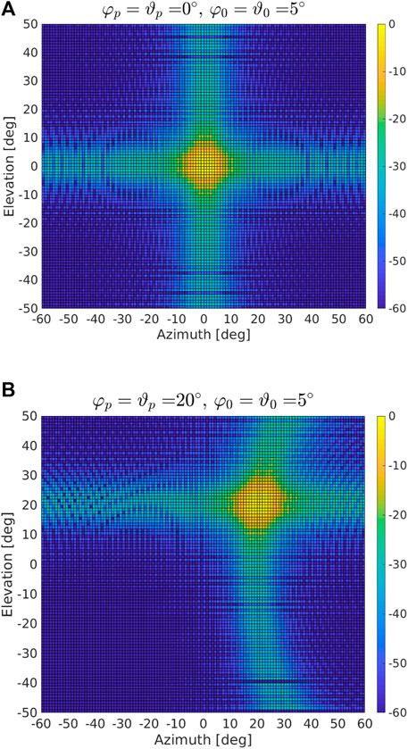
FIGURE 2. Radiation pattern [dB] for the proposed strategy obtained through w with a two-side aperture of 10°: (A) φp = ϑp = 0°, (B) φp = ϑp = 20°.
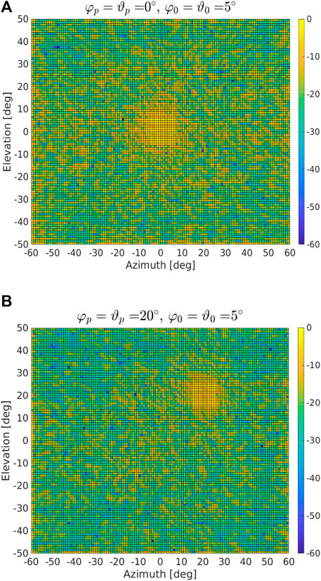
FIGURE 3. Radiation pattern [dB] for the GPA obtained through
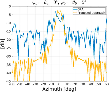
FIGURE 4. Cuts at 0° elevation for the GPA and the proposed approach assuming a two-side aperture of 10° and φp = ϑp = 0°.
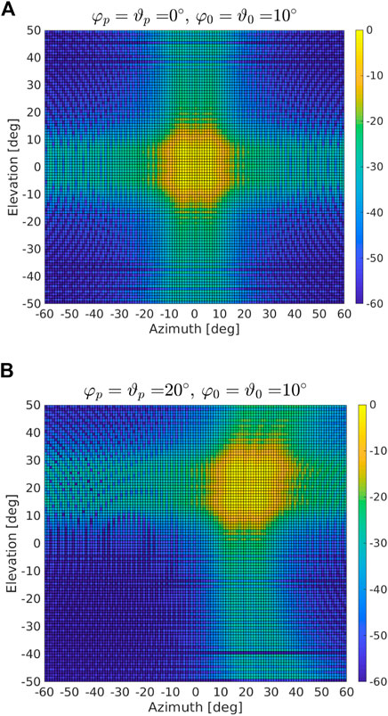
FIGURE 5. Radiation pattern [dB] obtained through w with a two-side aperture of 20°: (A) φp = ϑp = 0°, (B) φp = ϑp = 20°.
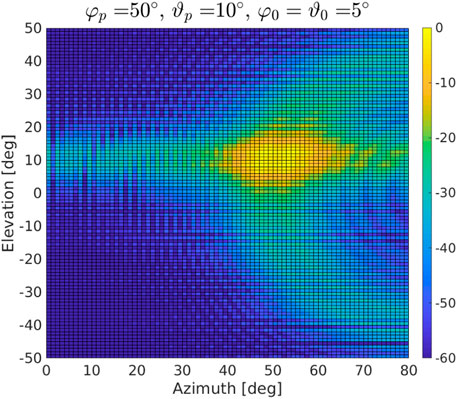
FIGURE 6. Radiation pattern [dB] obtained through w with a two-side aperture of 5°, φp = 50°, and ϑp = 10°.
To provide a more quantitative analysis, in Figure 7 we show different elevation cuts (along azimuth) assuming φp = ϑp = 20° and φ0 = ϑ0 = 5° in Subfigure 7a while φp = ϑp = 0° and φ0 = ϑ0 = 10° in Subfigure 7b. From the inspection of the figure, we notice that there exists a “transition band” of about 15° with a “stopband” that is about 30 dB below the “passband” when φ0 = ϑ0 = 5° and 25 dB when φ0 = ϑ0 = 10°. Moreover, the ripple extension in the mainlobe is less than 5 dB in both cases.
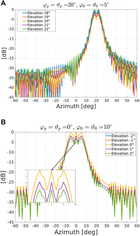
FIGURE 7. Azimuth cuts at different elevations [dB] obtained through w: (A) φp = ϑp = 20° and φ0 = ϑ0 = 5°, (B) φp = ϑp = 0° and φ0 = ϑ0 = 10°.
In Figure 8, we show the effects of quantization on the beam formation (0° elevation cut). Specifically, we uniformly quantize the real and imaginary parts of the beamformer weights with a dynamic range given by [−1, 1]. In the figure, the uniform quantizer considers Nb = 2, 4, 6, 8 bits and we set φ0 = ϑ0 = 5° and φp = ϑp = 0°. It can be noticed that for Nb = 2 the peaks of the sidelobes are in between [−25, − 20] dB against the original values that are around −37.5 dB. Nevertheless, for Nb = 4, the peaks of the sidelobe levels are in between −35 dB and −30 dB and follow more strictly the original evolution for Nb > 4. This behavior is confirmed by the inspection of Figure 9 that contains the magnitude histograms of the sidelobe regions for the considered sets of bits. Specifically, the “sidelobe region” is defined as the entire angular region of interest except for the set of angles within [−15°, 15°] × [−15°, 15°]. The root mean square errors (computed by averaging over the considered pointing directions) between the 2-dimensional original and quantized patterns are shown in Table 1. It turns out that the error values are quite low and, as expected, decrease when the number of quantization levels grows. On the other hand, widening the beam leads to an increase of the error.
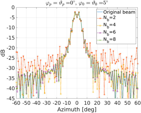
FIGURE 8. Radiation pattern along azimuth (0° elevation cut) for different quantization levels.
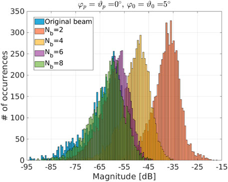
FIGURE 9. Magnitude histograms of the sidelobes’ region.
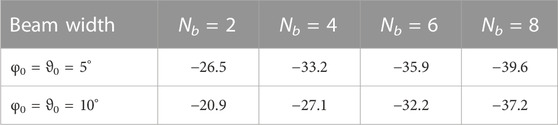
TABLE 1. RMSE values [dB] due to quantization.
4 Conclusion
In this paper, we have shown that an arbitrarily wide and almost flat beam can be obtained by exploiting the Fourier transform of LFM complex signals. To this end, we had to derive the connection between the LFM signal parameters and the beam width to achieve the straightforward tuning of the beam shape. The proposed method has a significant practical value since it does not resort to time-demanding optimization procedures. The illustrative examples have shown that the proposed method can give rise to beams whose width can be efficiently controlled by suitable tuning parameters, i.e., φ0, ϑ0, φp, and ϑp. More importantly, it exhibits better sidelobes properties than the iterative competitor and its computational requirements are significantly lighter than those related to the iterative competitor that launches a cyclic procedure for each pointing direction in the region of interest.
Future research tracks might encompass the investigation of illumination functions leading to different beam shapes under the required constraints or the experimentation of the proposed method on real radar systems with more populated array aperture.
Data availability statement
The original contributions presented in the study are included in the article, further inquiries can be directed to the corresponding author.
Author contributions
All authors listed have made a substantial, direct, and intellectual contribution to the work and approved it for publication.
Conflict of interest
The authors declare that the research was conducted in the absence of any commercial or financial relationships that could be construed as a potential conflict of interest.
The author(s) declared that they were an editorial board member of Frontiers, at the time of submission. This had no impact on the peer review process and the final decision.
Publisher’s note
All claims expressed in this article are solely those of the authors and do not necessarily represent those of their affiliated organizations, or those of the publisher, the editors and the reviewers. Any product that may be evaluated in this article, or claim that may be made by its manufacturer, is not guaranteed or endorsed by the publisher.
Footnotes
1It is important to highlight that different covering grids can be considered.
References
Alhujaili, K., Monga, V., and Rangaswamy, M. (2019). Transmit MIMO radar beampattern design via optimization on the complex circle manifold. IEEE Trans. Signal Process. 67 (13), 3561–3575. doi:10.1109/tsp.2019.2914884
Angeletti, P., Berretti, L., Maddio, S., Pelosi, G., Selleri, S., and Toso, G. (2022). Phase-only synthesis for large planar arrays via zernike polynomials and invasive weed optimization. IEEE Trans. Antennas Propag. 70 (3), 1954–1964. doi:10.1109/tap.2021.3119113
Cong, Y., Xiao, X., Zhong, K., and Hu, J. (2022). The phase only beamforming synthesis via an accelerated coordinate descent method. Digit. Signal Process. 128, 103624. doi:10.1016/j.dsp.2022.103624
Demir, O. T., and Tuncer, T. E. (2014). “Optimum discrete phase-only transmit beamforming with antenna selection,” in 2014 22nd European Signal Processing Conference (EUSIPCO), Lisbon, Portugal, September 1-5, 2014, 1282–1286.
Farina, A. (1992). Antenna-based signal processing techniques for radar systems. Boston, MA: Artech House.
Gershman, A. B., Sidiropoulos, N. D., Shahbazpanahi, S., Bengtsson, M., and Ottersten, B. (2010). Convex optimization-based beamforming. IEEE Signal Process. Mag. 27 (3), 62–75. doi:10.1109/msp.2010.936015
Hatam, M. (2022). “Phase-only array antenna beamforming with minimum peak sidelobe level and minimum power loss criteria,” in 2022 30th International Conference on Electrical Engineering (ICEE), Seoul, Korea, June 28 to July 2, 2022, 989–993.
Kautz, G. (1999). Phase-only shaped beam synthesis via technique of approximated beam addition. IEEE Trans. Antennas Propag. 47 (5), 887–894. doi:10.1109/8.774152
Liu, Y., Jiu, B., and Liu, H. (2020). ADMM-based transmit beampattern synthesis for antenna arrays under a constant modulus constraint. Signal Process. 171, 107529. doi:10.1016/j.sigpro.2020.107529
Mailloux, R. (2018). Phased Array Antenna Handbook, ser. Artech House antennas and electromagnetics analysis library. London, United Kingdom: Artech House.
W. L. Melvin (Editor) (2012). Principles of modern radar: Advanced techniques, ser. Radar, sonar and navigation (Delhi, India: Institution of Engineering and Technology).
Melvin, W., and Scheer, J. (2013). Principles of modern radar: Radar applications, volume 3, ser. Electromagnetics and radar. Delhi, India: Institution of Engineering and Technology.
Oppenheim, A., and Schafer, R. (1975). Digital Signal Processing, ser. Prentice Hall international editions. Hoboken, New Jersey: Prentice-Hall.
Pallotta, L., Farina, A., Smith, S. T., and Giunta, G. (2021). Phase-only space-time adaptive processing. IEEE Access 9, 147 250–147 263. doi:10.1109/access.2021.3122837
Papoulis, A. (1977). Signal Analysis, ser. Electrical & electronic engineering series. New York, United States: McGraw-Hill.
Richards, M. (2014). Fundamentals of radar signal processing. 2. New York, United States: McGraw-Hill Education.
Rixon Fuchs, L., Maki, A., and Gällström, A. (2022). Optimization method for wide beam sonar transmit beamforming. Sensors 22 (19), 7526. doi:10.3390/s22197526
Skolnik, M. (2001). Introduction to Radar Systems, ser. Electrical engineering series. New York, United States: McGraw-Hill.
Stutzman, W., and Thiele, G. (2012). Antenna Theory and design, ser. Antenna theory and design. Hoboken, New Jersey: Wiley.
Sun, S., and Li, H. (2003). “Simplified beamforming on phase-only arrays,” in Proceedings of the 2003 International Conference on Neural Networks and Signal Processing, Istanbul, Turkey, June 26 - 29, 2003, 1290–1293.
Tranter, J., Sidiropoulos, N. D., Fu, X., and Swami, A. (2017). Fast unit-modulus least squares with applications in beamforming. IEEE Trans. Signal Process. 65 (11), 2875–2887. doi:10.1109/tsp.2017.2666774
Tranter, J., Sidiropoulos, N. D., Fu, X., and Swami, A. (2016). “Fast unit-modulus least squares with applications in transmit beamforming,” in 2016 24th European Signal Processing Conference (EUSIPCO), Budapest, Hungary, August 29-September 2, 2016, 1378–1382.
Webster, T., Higgins, T., Shackelford, A. K., Jakabosky, J., and McCormick, P. (2015). “Phase-only adaptive spatial transmit nulling,” in 2015 IEEE Radar Conference (RadarCon), Arlington, Virginia, 10-15 May 2015, 0931–0936.
Keywords: beamforming, complex-valued linear frequency modulated signal, flat beam, phase-only beamforming, radar, transmitter module saturation
Citation: Orlando D and Farina A (2023) Phase-only array transmit beamforming without iterative/numerical optimization methods. Front. Sig. Proc. 3:1244530. doi: 10.3389/frsip.2023.1244530
Received: 22 June 2023; Accepted: 01 August 2023;
Published: 17 August 2023.
Edited by:
Fabio Dell’Acqua, University of Pavia, ItalyReviewed by:
Ming Zhang, Xi’an Jiaotong University, ChinaBrian Ng, University of Adelaide, Australia
Copyright © 2023 Orlando and Farina. This is an open-access article distributed under the terms of the Creative Commons Attribution License (CC BY). The use, distribution or reproduction in other forums is permitted, provided the original author(s) and the copyright owner(s) are credited and that the original publication in this journal is cited, in accordance with accepted academic practice. No use, distribution or reproduction is permitted which does not comply with these terms.
*Correspondence: Danilo Orlando, ZGFuaWxvLm9ybGFuZG9AdW5pY3VzYW5vLml0