4DEgo: ego-velocity estimation from high-resolution radar data

Automotive radars allow for perception of the environment in adverse visibility and weather conditions. New high-resolution sensors have demonstrated potential for tasks beyond obstacle detection and velocity adjustment, such as mapping or target tracking. This paper proposes an end-to-end method for ego-velocity estimation based on radar scan registration. Our architecture includes a 3D convolution over all three channels of the heatmap, capturing features associated with motion, and an attention mechanism for selecting significant features for regression. To the best of our knowledge, this is the first work utilizing the full 3D radar heatmap for ego-velocity estimation. We verify the efficacy of our approach using the publicly available ColoRadar dataset and study the effect of architectural choices and distributional shifts on performance.

1 Introduction

Automotive radars have gained significant attention in recent years. New 76–81 GHz high-resolution sensors (Dickmann et al., 2016; Engels et al., 2017) have shown potential for tasks beyond obstacle detection and velocity adjustment. Unlike traditional automotive radars, they can be used for localization (Heller et al., 2021), SLAM (simultaneous localization and mapping) (Holder et al., 2019), and ego-motion estimation. The estimation of ego-motion can enable other higher-level tasks such as mapping, target tracking, state estimation for control, and planning (Steiner et al., 2018). The majority of ego-motion and odometry algorithms relies on onboard sensors like IMU cameras and lidar. Vision-based methods use a stream of images acquired with single or multiple cameras attached to the robot for relative transformation (rotation and translation) estimation (Yang et al., 2020). Lidar has been well explored for these tasks in recent years and performs extremely well for odometry/ego-motion estimation. Classical lidar-based odometry methods (Zhang and Singh, 2014; Shan et al., 2020; Shan and Englot, 2018) use ICP (iterative closest point) (Besl and McKay, 1992) and NDT (normal distributed transform)-based registration (Magnusson et al., 2007; Zhou et al., 2017).

Despite such advances, optical sensors like cameras and lidar have become unreliable in visually degraded environments and adverse weather. Automotive radars operate on millimeter wavelengths, and their emitted radio signal does not degrade much in the presence of dust, smoke, or adverse weather conditions. The frequency modulation features a sensor to be used in multiple intrinsic settings to adjust the range and field of view. Radar data are different from lidar point clouds and camera data and are collected as complex value tensors (Engels et al., 2017), as shown in Figure 2. Because of its complex nature, interpreting these data is not trivial. In this study, we converted the raw data to a so-called “heatmap” before registration. Figure 3 visualizes one radar scan in a three-dimensional radar heatmap, which is data intensity versus range–azimuth–elevation. A bird's-eye view of this heatmap is shown in Figures 1, 4.

FIGURE 1

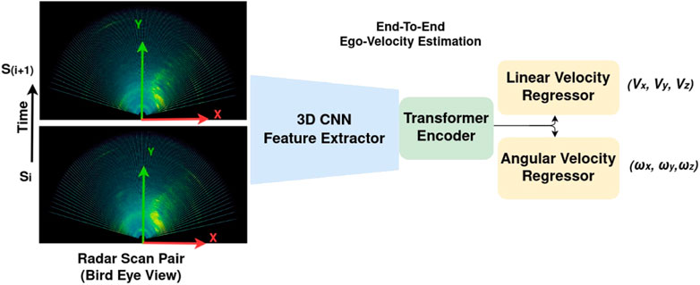
FIGURE 1. Proposed method for estimating the linear and angular velocities from consecutive radar scans (S_i, S_i+1). The feature extractor is a 3DCNN, which learns the features from the scans; further features are passed to a transformer encoder, and then, a set of linear and angular velocities is obtained via regression.

A major challenge of radar data is the noise that hinders hand-crafted feature extraction and semantic understanding of the signals. Several post-processing algorithms for radar point clouds have been proposed, such as CFAR (constant false alarm rate) (Rohling, 1983), which is primarily used in obstacle detection and avoidance. CFAR relies on the identification of high-intensity regions in the heatmap scans and applies a sliding window-based thresholding approach to select these regions. Methods like CFAR are better suited for detecting moving objects but often overlook small static objects due to their low reflectivity. However, when it comes to ego-motion estimation, it is crucial to not suppress the features of static targets. Therefore, this paper used high-resolution heatmaps as input for an end-to-end learning-based approach for ego-velocity estimation. We did this by learning a transformation (angular and linear velocities) between the consecutive pairs of 3D radar heatmaps. This method used a 3D convolutional neural network (3DCNN) (Tran et al., 2014) to extract the features associated with the objects in radar scans. A decoder network later performed the ego-velocity regression based on the feature matching across the pairs of scans, as illustrated in Figure 1 and explained in Section 3.2. The major advantage of our method is that we do not select features by hand; our network learns them by using pose trajectory ground truth. The contributions of this paper can be summarized thus:

• Using the full 3D radar heatmap scans for ego-motion estimation for scan-to-scan registration. The majority of current state-of-the-art methods seem to use radar point clouds, hand-crafted features, or additional sensors.

• We propose an end-to-end ego-velocity estimation architecture, which includes a 3D convolution over all three channels of the heatmap scan to capture features associated with the motion and an attention mechanism for selection of the significant features for regression. Our method achieves 0.037 m/s RMSE (root mean squared error) in linear forward speed and 0.048 deg/s in heading angle rate, tested on the publicly available ColoRadar dataset (Kramer et al., 2022).

• We investigate the effect of ego-velocity regressor architecture through extensive experiments on different environments and speeds. We compare several alternatives for regressor architecture: without attention, transformer encoder, self-attention, and channel attention. In two of the selected results, we show that a) RMSE error increases by only 5% in the test environment compared to the training environment, while b) the error increases by 90% for higher-speed test data.

The paper is organized thus: Section 2 presents the related work; Section 3 includes problem formulation and network architecture details; radar data format, heatmap processing, ground truth calculation, and training are introduced in Section 4; evaluation of models and result comparison are discussed in Section 5; Section 6 concludes and suggests future work.

2 Related work

Radar has long been a sensor of choice for emergency braking and obstacle detection due to its capability of perception in visually degraded environments, such as bad weather (rain, fog, and snowfall), darkness, dust, and smoke. Initial research with automotive radars was conducted in the late 1990s (Clark and Durrant-Whyte, 1998); in the last several years, significant work has been conducted in radar-based odometry and SLAM (Daniel et al., 2017; Ghabcheloo and Siddiqui, 2018). Ego-motion estimation research predominantly focuses on two types of sensors: spinning radars and Doppler automotive radars (SoC radars).

2.1 Spinning radar

Spinning radars have been widely used for SLAM and odometry due to their high-resolution image-like data and 360° coverage. However, these radars are bulky (about 6 kg) and are not energy-efficient. They provide only 2D scans (azimuth and range) through 360 deg spatial coverage. Several spinning radar datasets (Barnes et al., 2020; Kim et al., 2020; Sheeny et al., 2020; Burnett et al., 2022) are available for benchmarking the state-of-the-art methods. These methods usually fall into two categories: learning-based and non-learning-based. The majority of non-learning-based methods perform descriptor selection from image-like radar scans, followed by registration across consecutive frames. In an ego-motion estimation study, Cen and Newman (2018) used scan matching with hand-crafted feature points from radar scans. Adolfsson et al. (2021) proposed a method of selecting an arbitrary number of the highest intensity returns per azimuth, and, after oriented surface point calculation, registration was performed between the final key frame and the current frame. Some recent learning-based methods have extracted the key points end-to-end by self-supervised learning (e.g. Barnes et al., 2019). In Burnett et al. (2021), features were first learned in an unsupervised way, and then the feature extractor was combined with classical probabilistic estimators for ego-motion estimation.

2.2 SoC radar

SoC (system-on-chip) radars consume less power and are more lightweight than spinning radars. With the evolution of SoC radars over the past five years, new high-resolution sensors have been introduced. Modern radars provide 4D data (range, azimuth, elevation, and Doppler). With these radars, ego-motion estimation falls into two categories: instantaneous (single scan) and registration-based (multiple scans). Instantaneous ego-motion estimation relies on the Doppler velocity of targets in the scan and is solved through non-linear optimization (e.g. Kellner et al., 2013). The instantaneous approach cannot estimate 6DoF (three-dimensional linear and angular transformations) ego-motion from only one radar sensor. To solve full ego-motion, we need multiple radar sensors (minimum of two), as in Kellner et al. (2014), or an additional IMU (inertial measurement unit) sensor, as in Ghabcheloo and Siddiqui (2018). Another approach is to solve the ego-motion by registration across consecutive radar scans of a single radar sensor. For example, Almalioglu et al. (2021) used NDT registration (Magnusson et al., 2007) and an IMU-based motion model. All these methods operate on so-called radar point clouds that are pre-processed sparse radar points from the heatmaps. Pre-processing is performed, for example, by CFAR or simple intensity thresholding. Our method, on the other hand, uses full radar heatmaps and performs ego-velocity regression. We also propose a novel network architecture that has a 3DCNN for feature extraction and attention layers for selecting significant features for ego-velocity regression.

Learning-based methods for ego-motion estimation have emerged in recent years with the evolution of deep neural networks. State-of-the-art research has shown better performance than the classical methods for ego-motion estimation, optical-flow estimation, and SLAM front-end. MilliEgo (Lu et al., 2020) is an end-to-end approach for solving radar-based odometry. Its methodology differs from ours in several aspects: 1) milliEgo takes the radar point cloud as an input, which suppresses some useful information from the heatmap; 2) our network architecture is very different in terms of feature extraction and regression; 3) milliEgo has only been evaluated indoors, while we provide evaluation on an indoor-to-outdoor and low-speed-to-high-speed dataset; 4) milliEgo uses three single chip radar sensors (Li et al., 2022), while our sensor is a high-resolution TI AWR2243 (four-chip cascade radar; 5) milliEgo uses an additional IMU sensor.

3 Methodology

This section starts with problem formulation in 3.1, where we formalize the ego-motion problem and introduce the loss function for supervised learning, and 3.2 explains the network architecture, including the feature extractor and ego-velocity regressor shown in Figure 4.

3.1 Problem formulation

The ego-motion of a frame attached to a moving body is the change in transformation T = (R, t), rotation, and translation, respectively, over time with respect to a fixed frame. We used angular and linear 6-DoF twist (V = [V_x, V_y, V_z], ω = [ω_x, ω_y, ω_z]) to represent ego-motion. We solved this problem by using registration—geometrically aligning two radar scans, which are in the form of intensity heatmaps. To solve the registration problem, we trained a model that takes as input two consecutive radar heatmaps (S_i, S_i+1) (Figure 1) and outputs the predictions of the linear and angular velocities $(\widehat{V},\widehat{\omega })$ as follows:

$\widehat{V},\widehat{\omega }=\mathcal{F}\left(\left(S_i,S_{i+1}\right);\theta \right),(1)$

where $\mathcal{F}$ is a neural network with parameters θ.

Our neural network is composed of an encoder (3DCNN feature extractor) and an ego-velocity regressor network D (Figure 1). Details of the network architecture are given in Section 3.2. The objective of the training is to find the set of parameters θ that minimizes the distance between the network output $(\widehat{V},\widehat{\omega })$ and the ground truth velocities (V, ω) using the following loss:

$Loss=\frac{1}{N}{\displaystyle \sum _{i\in S}}{w}_1\Vert V_i-\widehat{V_i}{\Vert }_2^2+w_2\Vert {\omega }_i-\widehat{{\omega }_i}{\Vert }_2^2,(2)$

where S is the dataset and N = |S| is the number of training data samples. Each sample includes a pair of heatmaps and a ground truth velocity vector. Scalar values w₁ and w₂ are weighting factors to balance the linear and angular regression portion of the loss.

3.2 Network architecture

The network architecture is illustrated in Figure 4. It is composed of two main building blocks: a 3DCNN feature extractor and an ego-velocity regressor block. To estimate the ego-motion for a given pair, we needed to perform feature matching between consecutive radar heatmaps. Feature matching is the process of identifying corresponding features between two radar heatmaps. Corresponding features are those that represent the same region of interest (salient area with higher intensity) being tracked in both heatmaps. CNN is capable of learning features in the form of patches, corners, and edges. A fully connected regressor network can perform descriptor (feature vector) matching by finding the closest match from one heatmap to the other in the pair based on geometry (Euclidean distance in our case) (Wang et al., 2017) (Costante et al., 2016). By incorporating the transformer encoder in the ego-velocity regressor, we enhance the feature matching process for more accurate ego-motion estimation. Details of the network architecture are explained in 3.2.1 and 3.2.2.

3.2.1 Feature extraction

Our input data are three-dimensional, with intensity along three axes: range (128), azimuth (128), and elevation (32). We thus use a 3DCNN-based feature extractor to handle these data. Here, our feature extractor takes a pair of radar heatmaps in Cartesian form and generates the feature vector for use by the ego-velocity regressor. This network has nine convolutional layers, where the number of convolutional filters varies from 64 to 1024. Filter sizes for the first two layers are (7 × 7 × 7) and (5 × 5 × 5) and for the remaining layers is (3 × 3 × 3). The varying size of the filter helps the network learn the large- and small-scale features. We denote a feature vector obtained from the pair of scans by f. The dimension of f for each batch is (1,2,2,1024), and it is passed further to a regressor block for further processing.

3.2.2 Feature refinement and regression

The ego-velocity regressor block comprises a feature refinement block (referred to as the “Transformer Block” in Figure 4), and a dual-head fully connected decoder (FC decoder). Each decoder head has three layers, and the last layer gives the final output as a vector of three elements. In the feature refinement block, we tested the following attention (Vaswani et al., 2017) strategies:

• 3DCNN + SA + FC, where “SA” is self-attention;

• 3DCNN + CA + FC, where “CA” is channel attention;

• 3DCNN + Transformer + FC, where “Transformer” is transformer encoder;

• 3DCNN + FC, a model without attention.

The attention mechanism assigns higher weights to significant features in comparison to other features of the feature vector obtained from the 3DCNN feature extractor. In the following paragraphs, we provide details of the tested attention strategies.

3DCNN + Transformer + FC: Transformers benefit from multi-head attention and have shown better performance than CNN on vision tasks (Dosovitskiy et al., 2021). Multi-head attention learns the local and global features from the input feature vector concatenated with the attention mask. We use the transformer encoder layers TransEnc with positional encoding PE; these select significant and stable features with their local and global context from the input feature vector. Since our input is one instance of an input pair, we follow positional encoding similar to Dosovitskiy et al. (2021), which is applied only to spatial dimensions. The positional encoding takes the feature vector of an input heatmap pair and generates the positional information for features in the input feature vector. The output of positional encoding PE is added element-wise to the feature vector, which is further passed through two transformer encoder layers (Figure 4). Each of the transformer encoder layers has eight multi-head attention units, a layer normalization LayerNorm, a max pooling MaxPool layer (for aggregating and preserving contextual information associated with the features), and an activation function. The output feature vector from the transformer encoder f_out is passed through the FC dual-head velocity regressor.

$f_{\mathit{out}}=MaxPool\left(LayerNorm\left(TransEnc\left(PE\left(f\right)+f\right)\right)\right).(3)$

3DCNN + SA + FC: For the self-attention mechanism, we use the same attention technique as in Lu et al. (2020). The purpose of self-attention is to focus on stable and geometrically meaningful features rather than noisy and less stable features. Applied to the features obtained from the 3DCNN, this method performs global average pooling AvgPool to aggregate the features and outputs an attention mask. The attention mask will further be multiplied with the feature input through an element-wise multiplication operator ⊗. Denoting the number of channels in the feature vector (corresponding to the elevation dimension in the heatmap) by c, a dense layer with rectified linear unit activation by MLP and the self-attention by MLP, f_out is computed using the following equations:

$S^{1\times 1\times c}=MLP\left(AvgPool\left(f\right)\right),(4)$

$f_{\mathit{out}}=S\otimes f.(5)$

3DCNN + CA + FC: Channel attention was proposed in Woo et al. (2018). For a given feature vector, channel attention generates the attention mask across all channels and learns rich contextual information with the help of max pooling MaxPool. It still uses AvgPool for aggregating spatial information in addition to learning their context. It is a lightweight attention module that is used for 3DCNN feature refinement. C is the channel attention mask, and f_out is computed as follows:

$C^{1\times 1\times c}=\sigma \left(MLP\left(AvgPool\left(f\right)\right)+MLP\left(MaxPool\left(f\right)\right)\right).(6)$

σ is the sigmoid function for keeping the values between 0 and 1 in the attention mask.

$f_{\mathit{out}}=C\otimes f,(7)$

where ⊗ is the element-wise multiplication between the attention mask and the feature vector f.

FC decoder: The final feature vector f_out is passed to the two regressor blocks D₁ and D₂ for linear and angular velocity regression:

$\widehat{V}=D_1\left(f_{\mathit{out}}\right),(8)$

$\widehat{\omega }=D_2\left(f_{\mathit{out}}\right).(9)$

4 Experiments

In this section, we explain the data in 4.1, raw data format and sensor details in 4.2, the process of heatmap generation in 4.3, ground truth calculation in 4.4, and model training in 4.5.

4.1 Data

We evaluated our models on the ColoRadar (Kramer et al., 2022) dataset that was recorded in seven different indoor and outdoor environments with a hand-carried sensor rig for the tasks of localization, ego-motion estimation, and SLAM. The ColoRadar dataset has a total of 57 sequences. The sensor rig included a high-resolution radar, a low-resolution radar, a 3D Lidar, an IMU, and a Vicon motion capture system for indoors. Radar was mounted front-facing where (x = azimuth, y = range, z = elevation). The authors provided ground truth poses (position and orientation) in the body (sensor rig) frame, generated by a 3D lidar-IMU-based SLAM package (Hess et al., 2016). Ground truths were provided as pose trajectory with timestamp for each sequence. The data are organized in Kitti format (Geiger et al., 2013), where the sensor readings and the ground truth poses are stored with their timestamps for each data sequence. We used the high-resolution radar data with the ground truth poses from the dataset. We used a subset of the data specified in Table 1 for this experiment.

TABLE 1

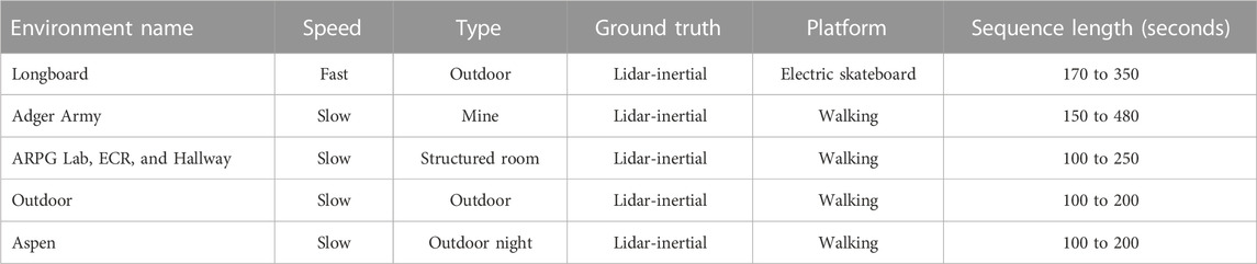
TABLE 1. ColoRadar data sequences used in our experiments.

4.2 Radar sensor and raw data format

Radar data were collected with a high-resolution sensor (TI-MMWAVE Cascade AWR2243 (Swami et al., 2017))—FMCW (frequency-modulated continuous wave) radar. It has three vertically placed elevation transmitter antennas with nine horizontal azimuth transmitter antennas to cover a three-dimensional field of view. It has 16 receiver antennas to receive the reflected signal from objects and landmarks in the environment. This sensor has a field-of-view of 140° in azimuth and 45° in elevation. It has an angular resolution of 1° in azimuth and 15° in elevation. As Figure 2 illustrates, the transmitters transmit the set of N electromagnetic signals known as chirps in each frame. Within each frame, the transmitted signal increases linearly with time from starting f_c to maximum frequency f_c + B, where B is the bandwidth. Each chirp is sampled in time by the time difference T_s, or “fast time dimension”. Receivers receive the reflected signal by a time delay t, which is used to calculate the range of reflector. In each radar frame, the data are stored as a two-dimensional matrix of samples and chirps (number of chirps in the frame known as slow time dimension) for each receiver antenna. We get a three-dimensional (samples, chirps, and receivers) complex value tensor as raw data—also known as “ADC (analog-to-digital converted) data”. In FMCW radars, spatial resolution of sensors is limited by the number of receiver antennas. To achieve better spatial resolution in azimuth and elevation without adding more physical antennas, a MIMO (multiple input—multiple output) technique is used in modern radars. MIMO created a virtual receiver array of size (number of transmitters × number of receivers) (Engels et al., 2017) for high-resolution angle estimation, with the output data dimensions becoming (samples, chirps, number of transmitters × number of receivers).

FIGURE 2

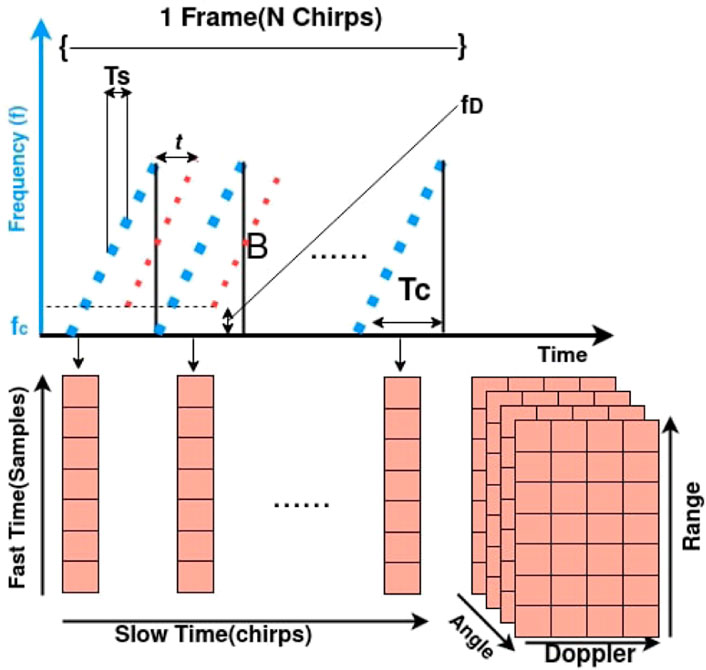
FIGURE 2. Raw radar data formation for a given frame; details explained in 4.2. In each frame are transmitted chirps (blue dotted line, dots as samples) and received chirps (red lines). Received samples organized for each receiver by running FFT along fast time give us range and along slow time give us Doppler. We get angles by running FFT on receiver dimension.

4.3 3D heatmap processing

The first step was to perform calibration in phase and frequency to address the mismatch caused by four radar transceivers on the cascade board. Calibration parameters vary from sensor to sensor, and the dataset has those parameters provided. We performed the calibration with the existing ColoRadar development toolkit.

After the calibration, we performed the post-processing using fast Fourier transforms in range, Doppler, and angle dimensions with a velocity compensation algorithm to avoid Doppler ambiguity caused by the movement of the radar in MIMO (Bechter et al., 2017). In post-processing, the MIMO ADC data are passed to a two-dimensional fast Fourier transform to obtain the range-Doppler heatmap, followed by a phased array angle processing module to obtain the azimuth and elevation. The processed data were organized into discrete 3D bins with two values for each bin (intensity and Doppler velocity). We do not use the Doppler velocity in the input data. The scan dimensions are (elevation = 32, azimuth = 128, range = 128), which are the parameter settings used to collect the dataset (Kramer et al., 2022). A heatmap scan is shown in Figure 1, representing the bird's-eye view (top view) of the 3D heatmap shown in Figure 3. Figure 3 shows the heatmap data for all elevation layers with range and azimuth.

FIGURE 3

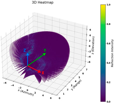
FIGURE 3. 3D heatmap data: here, higher reflection intensities show the regions with possibility of landmarks (Cartesian plot (range, azimuth, and elevation are in meters) for simple visualization).

4.4 Ground truth calculation

The dataset provided ground-truth poses in the sensor rig frame at a frame rate of 10 FPS. To perform radar-based ego-motion estimation, the ground truth needed to be in the radar sensor frame. Since radar has a lower data frequency (5 FPS), we located the ground-truth instances for the radar timestamps and converted them from the body frame to the sensor frame using the static transform provided in the dataset.

We then use the following equation (see (Lynch and Park, 2017) for more details) to calculate ground-truth twist from consecutive pose transformations:

$\left[\begin{array}{cc}\hfill \left[{\omega }_i\right]\hfill & \hfill V_i\hfill \\ \hfill 0\hfill & \hfill 1\hfill \end{array}\right]=T{\left(i\right)}^{-1}\dot{T}\left(i\right),(10)$

where T(i) is the transformation at time index i and [ω_i] is the skew symmetric matrix containing the angular velocity. $\dot{T}(i)$ is the time derivative of T(i) and is calculated approximately using $\dot{T}(i)=(T(i+1)-T(i))/dt$.

4.5 Training

We used a pair of radar heatmaps as training samples and corresponding linear and angular velocities as ground truth. While processing the data for training, we kept the samples in temporal order using the timestamps for each sequence. All the input ground-truth labels have been normalized between 0 and 1 for stable network training. We trained four networks (as described in Section 3): 3DCNN + FC, 3DCNN + SA + FC, 3DCNN + CA + FC, and 3DCNN + Transformer + FC. These networks have been trained on the same dataset with similar hyperparameters. They were trained for 50 epochs on the Nvidia RTX 3080 platform with Adam optimizer (Kingma and Ba, 2014) and learning rate 10^–4. We chose 8000 heatmap pairs from four environments. From these samples, we chose 80% data for training and rest for validation and testing (10% each). In the feature extractor, we used dropout (Srivastava et al., 2014) (0.2 until eighth layer, 0.5 in last layer) in all layers to avoid overfitting by randomly dropping the weights. For stable and faster training, we used batch normalization in the 3DCNN (Ioffe and Szegedy, 2015) in each layer. We also used LeakyReLu (Xu et al., 2015) with 0.01 hyperparameter as an activation function in layers. This activation function is good for avoiding the vanishing gradient problem in network architecture with a higher number of layers. The number of parameters and layers for our ego-velocity regressor and models with attention mechanism are explained in 3.2.2 and shown in Figure 4. We chose a small subset of data and did not use the whole dataset.

FIGURE 4

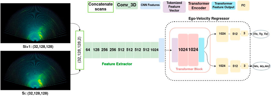
FIGURE 4. Proposed method for estimating linear and angular velocities from consecutive radar scans (S_i, S_i+1); each radar scan has intensity values distributed in 3D space (el = elevation, az = azimuth, and r = range). Feature extractor is 3DCNN, which learns the features from the radar data; these features are passed to a transformer encoder and then to a set of linear and angular velocities obtained through an ego-velocity regressor.

5 Results

We used the following training datasets in our experiments:

• Mixed data: indoor structured (two sequences), indoor unstructured (one sequence), and outdoor (one sequence), low speed

• Indoor data: indoor structured (two sequences) and indoor unstructured (one sequence)

and RMSE (root mean squared error) metric, defined by

$RMSE=\sqrt{\frac{{\mathrm{\Sigma }}_{i=1}^N{\left(X_{\mathit{pred}}-X_{gt}\right)}^2}{N}},(11)$

where N is the number of the data samples. We calculate the RMSE for each element of the twist separately. In the tables, the linear velocity (V_x, V_y, V_z) errors are in meter per second, and the angular velocity (ω_x, ω_y, ω_z) errors are in degree per second.

We evaluated our models with the following experiments:

• Trained and tested on mixed data: results reported in Table 2 and explained in Section 5.1

• Trained and tested on mixed–tested stationary and moving separately: results in Tables 5 and 4, and explained in 5.2

• Trained on mixed low speed–tested on mixed high speed: results in Table 6 and explained in 5.3.2

• Trained on indoor data–tested on outdoor data: results in Table 3 and explained in 5.3.1

TABLE 2

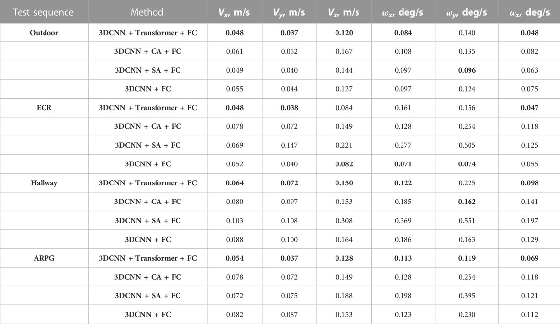
TABLE 2. Average RMSE errors for each test sequence (trained and tested on the mixed dataset). Smallest errors per sequence are marked in bold.

TABLE 3

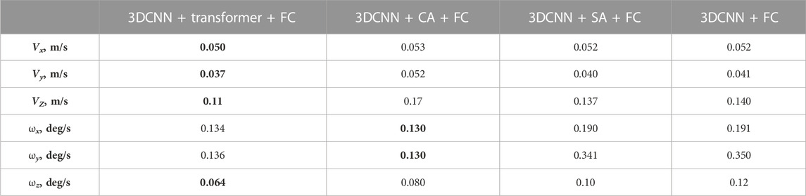
TABLE 3. Generalization test (performance of models trained on indoor data and tested on distribution data, outdoor night sequence (Aspen)). Smallest errors per velocity component are marked in bold.

The results of these experiments are presented and discussed in the following paragraphs.

5.1 Trained and tested on mixed data

We took four sequences for evaluating the mixed (indoor + outdoor) training. Those sequences were selected from ARPG, ECR, Hallway, and outdoor environments. We chose three sequences for training and one for testing from each environment. We used the models trained on the mixed datasets; we ran each model on all four test sequences and compared the predicted values for all six ego-velocity components with the ground truth calculated (see Section 4.4). On Table 2, all four test sequences were collected by a person walking with the sensor rig. Sequence length for ARPG, Hallway, and outdoor environments is 100–120 s. ECR sequence length is 276 s. On the outdoor test sequence, significant differences were observed in the performance of models. From the results in Table 2, the model that uses transformer layers in the velocity regressor (3DCNN + Transformer + FC) provides a lower RMSE error than other models. In the other two indoor sequences—Hallway and ARPG—we also see similar performance. On the ECR sequence, where the indoor environment was different in structure and contained less training data, the transformer model (3DCNN + Transformer + FC) performed worse than other models for angular velocity components. We used boxplot for visualization, where the values are plotted as a distribution of errors in each element of ego-velocity for all models from Table 2; Figure 5 represents linear ego-velocities, and Figure 6 represents angular ego-velocities. These plots show the errors as boxes where mean values are shown as green triangles, the green line as median, and lower and upper boundaries show the standard deviation for each ego-velocity element. We observed that model C (3DCNN + SA + FC) clearly performs worse than other models for some velocity components. The main differences are for the velocity components that do not vary significantly across the selected dataset—for example, linear velocity in x and z dimensions (Vx, Vz) and angular velocity in x and y dimensions (ω_x, ω_y). Model C uses the simplest attention mechanism, just one layer of self-attention, and can thus cause more errors, especially when the actual values of ego-velocity components are small—for example, ω_y, ω_z < 0.5 deg/sec.

FIGURE 5

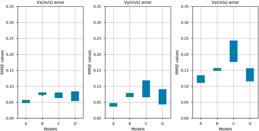
FIGURE 5. RMSE error distribution for each liner velocity component (trained and tested on the mixed dataset). Models include (A) 3DCNN + Transformer + FC, (B) 3DCNN + CA + FC, (C) 3DCNN + SA + FC, and (D) 3DCNN + FC). Each box accounts for errors from all four test sequences. The green line is the median, and green triangle is the mean value.

FIGURE 6

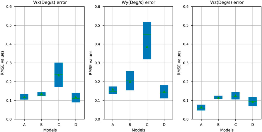
FIGURE 6. RMSE error distribution for each angular velocity component (trained and tested on the mixed dataset). Models include (A) 3DCNN + Transformer + FC, (B) 3DCNN + CA + FC, (C) 3DCNN + SA + FC, and (D) 3DCNN + FC). Each box accounts for errors from all four test sequences. The green line is the median, and the green triangle is the mean value.

5.2 Evaluation of static and dynamic parts of the sequence

In Section 5.1, we evaluated the whole length of the sequences. However, in each data sequence, the sensor platform was stationary for a short period at the beginning and end of the sequence. To test the accuracy of the models in the static and dynamic parts of sequence, we evaluated the models separately in two cases: 1) evaluating only the static part of the sequences where the sensor platform was not moving, and 2) evaluating the part of the sequences where the sensor platform was moving. Tables 4 and 5 present the results for the static and moving parts of the sequences, respectively. Results are reported as the mean and standard deviation of the RMSE for all four sequences. Results show that the static part prediction contained smaller errors than the moving part, where predictions have higher errors for all the models. In the case of the moving platform, the self-attention model (3DCNN + SA + FC) performed better than other models. However, in the static parts of the sequences, it predicts values with larger errors than other models. This experiment helps us understand the source of errors for the self-attention model in Section 5.1—the small values of velocity components having small variations in the training set.

TABLE 4

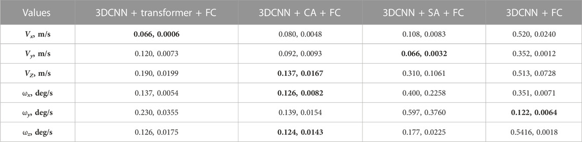
TABLE 4. Evaluation on only the static part of the sequence (performance of the models trained on indoor data and tested on mixed test sequences (indoor + outdoor), and mean and standard deviation of RMSE errors are presented). Smallest errors per velocity component are marked in bold.

TABLE 5

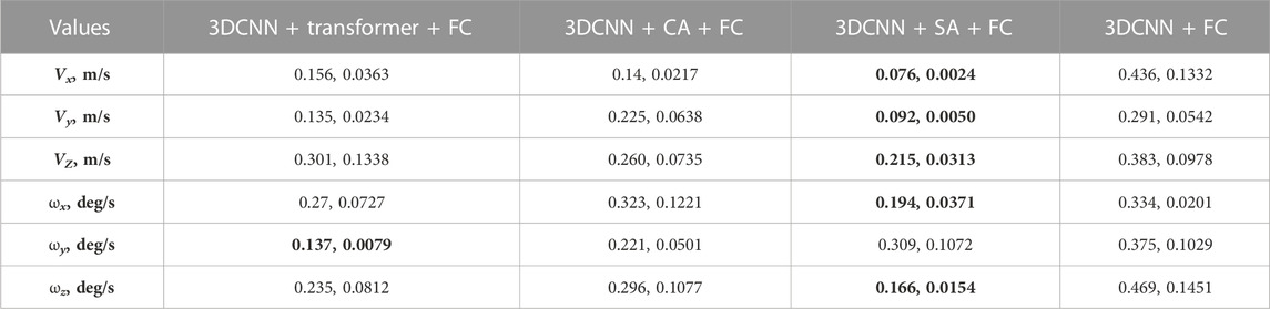
TABLE 5. Evaluation on only the moving part of the sequence (performance of models trained on indoor data and tested on mixed test sequences (indoor + outdoor), and mean and standard deviation of RMSE errors are presented. Smallest errors per velocity component are marked in bold.

5.3 Distribution shift

To evaluate the generalizability of the models, we tested two different distribution shifts: a) using a different environment for training and testing while maintaining the same sensor platform speed and b) utilizing a high-speed test sequence for the model trained on low-speed training data. We observed that changes in velocity pose significant challenges to generalization. However, we found that an environmental change has only minimal impact.

5.3.1 Trained on indoor data–tested on outdoor data

In the first distribution shift test, we assessed the models’ ability to generalize to a different environment. In this case, we trained the models using indoor data and tested them using an outdoor sequence. Table 3 presents the RMSE of all the models. The 3DCNN + Transformer + FC model demonstrated superior performance for all the velocity components except ω_x and ω_y, where 3DCNN + CA + FC performed slightly better. The results show little difference in errors compared to the mixed evaluation. This indicates that the models are not considerably impacted by the change in environment, implying that they have learned transferable features. This therefore indicates that the models have the ability to capture features that can be applied across different environments. Moving forward, we intend to investigate the utilization of these learned features for additional tasks such as mapping.

5.3.2 Trained on mixed low speed–tested on mixed high speed

In the second distribution shift test, the performance of the models trained on the mixed dataset was evaluated on a relatively high-speed test sequence. Note that all the mixed dataset sequences used in the training were low-speed (recorded while walking). The high-speed test sequence was collected by a person moving on an electric skateboard. Table 6 presents the results. None of the trained models showed satisfactory performance in this experiment. This result indicates that the models need retraining if they are to be used in scenarios with significantly different speeds or types of motion. Our model is learning the ego-motion based on the transformation between similar features extracted from a pair of heatmaps. In the higher-speed sequences, the platform travels greater distances between the instances of data, causing larger displacements between the features in the heatmap pairs. The dataset we used has only one environment with a higher platform speed, which is insufficient for training a model. Further exploration can be performed to train the models with self-supervised schemes for better generalization across different environments and varying speed settings.

TABLE 6

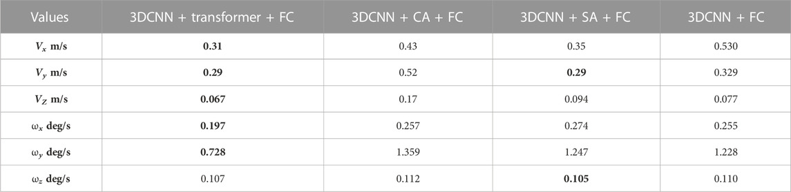
TABLE 6. Generalization test (performance of the models trained on low-speed data and tested on distribution data, high speed sequence (Longboard)). Smallest errors per velocity component are marked in bold.

6 Conclusion

We presented an end-to-end ego-velocity estimation method from high-resolution radar data. We avoided the heavy processing of radar data to obtain point clouds, which is computationally expensive and causes loss of useful information. Our proposed architecture consists of a 3DCNN based on FlowNet capturing the features associated with motion and an attention mechanism for the selection of significant features for regression. We tested three attention architectures and compared them with the option without attention, as explained in Section 5 We trained and evaluated the models on a subset of a publicly available ColoRadar dataset and studied the effect of distribution shift. Although the performance does not degrade greatly when transferring models from indoor to outdoor, the generalizability is rather poor in the varying speed experiment. Our training and evaluation settings have shown that use of transformer encoder layers can improve the performance of end-to-end radar-based ego-motion estimation using deep neural networks. It could be better with an increased amount of data. Future work will explore the applicability of this method in other high-level tasks like mapping and SLAM.

Data availability statement

The original contributions presented in the study are included in the article/supplementary material; further inquiries can be directed to the corresponding author.

Author contributions

Idea and conceptualization: PR and RG; experimental design and evaluation: PR and NS; data visualization and result representation: PR and NS; implementation: PR; draft writing: PR; final manuscript: PR, NS, and RG; supervision: RG and NS; funding acquisition, resources, and project administration: RG. All authors contributed to the article and approved the submitted version.

Funding

This project was supported by the European Union’s Horizon 2020 research and innovation program under the Marie Sklodowska-Curie grant agreement No. 858101 and by the Academy of Finland (project320 no. 336357, PROFI 6—TAU Imaging Research Platform).

Conflict of interest

The author declare that the research was conducted in the absence of any commercial or financial relationships that could be construed as a potential conflict of interest.

Author SR declared that they were an editorial board member of Frontiers at the time of submission. This had no impact on the peer review process and the final decision.

Publisher’s note

All claims expressed in this article are solely those of the authors and do not necessarily represent those of their affiliated organizations, or those of the publisher, the editors, and the reviewers. Any product that may be evaluated in this article, or claim that may be made by its manufacturer, is not guaranteed or endorsed by the publisher.

References

Adolfsson, D., Magnusson, M., Alhashimi, A., Lilienthal, A. J., and Andreasson, H. (2021). “Cfear radarodometry - conservative filtering for efficient and accurate radar odometry,” in IEEE/RSJ International Conference on Intelligent Robots and Systems (IROS). doi:10.1109/IROS51168.2021.9636253

CrossRef Full Text | Google Scholar

Almalioglu, Y., Turan, M., Lu, C. X., Trigoni, N., and Markham, A. (2021). Milli-rio: Ego-motion estimation with low-cost millimetre-wave radar. IEEE Sensors J. 21, 3314–3323. doi:10.1109/JSEN.2020.3023243

CrossRef Full Text | Google Scholar

Barnes, D., Gadd, M., Murcutt, P., Newman, P., and Posner, I. (2020). “The oxford radar robotcar dataset: A radar extension to the oxford robotcar dataset,” in IEEE International Conference on Robotics and Automation (ICRA).

CrossRef Full Text | Google Scholar

Barnes, D., Weston, R., and Posner, I. (2019). Masking by moving: Learning distraction-free radar odometry from pose information. ArXiv.

Google Scholar

Bechter, J., Roos, F., and Waldschmidt, C. (2017). Compensation of motion-induced phase errors in tdm mimo radars. IEEE Microw. Wirel. Components Lett. 27, 1164–1166. doi:10.1109/LMWC.2017.2751301

CrossRef Full Text | Google Scholar

Besl, P., and McKay, N. D. (1992). “A method for registration of 3-d shapes,” in IEEE Transactions on Pattern Analysis and Machine Intelligence. doi:10.1109/34.121791

CrossRef Full Text | Google Scholar

Burnett, K., Yoon, D. J., Schoellig, A. P., and Barfoot, T. D. (2021). “Radar odometry combining probabilistic estimation and unsupervised feature learning,” in Robotics: Science and systems (RSS).

Google Scholar

Burnett, K., Yoon, D. J., Wu, Y., Li, A. Z., Zhang, H., Lu, S., et al. (2022). Boreas: A multi-season autonomous driving dataset. arxiv preprint (2022).

Google Scholar

Cen, S. H., and Newman, P. (2018). “Precise ego-motion estimation with millimeter-wave radar under diverse and challenging conditions,” in IEEE International Conference on Robotics and Automation (ICRA). doi:10.1109/ICRA.2018.8460687

CrossRef Full Text | Google Scholar

Clark, S., and Durrant-Whyte, H. F. (1998). “Autonomous land vehicle navigation using millimeter wave radar,” in IEEE International Conference on Robotics and Automation(ICRA). doi:10.1109/ROBOT.1998.681411

CrossRef Full Text | Google Scholar

Costante, G., Mancini, M., Valigi, P., and Ciarfuglia, T. A. (2016). Exploring representation learning with cnns for frame-to-frame ego-motion estimation. IEEE Robotics Automation Lett. 1, 18–25. doi:10.1109/LRA.2015.2505717

CrossRef Full Text | Google Scholar

Daniel, L., Phippen, D., Hoare, E., Stove, A., Cherniakov, M., and Gashinova, M. (2017). “Low-thz radar, lidar and optical imaging through artificially generated fog,” in IET International Conference on Radar Systems.

CrossRef Full Text | Google Scholar

Dickmann, J., Klappstein, J., Hahn, M., Appenrodt, N., Bloecher, H. L., Werber, K., et al. (2016). “Automotive radar the key technology for autonomous driving: From detection and ranging to environmental understanding,” in IEEE Radar Conference (RadarConf). doi:10.1109/RADAR.2016.7485214

CrossRef Full Text | Google Scholar

Dosovitskiy, A., Beyer, L., Kolesnikov, A., Weissenborn, D., Zhai, X., Unterthiner, T., et al. (2021). “An image is worth 16x16 words: Transformers for image recognition at scale,” in International Conference on Learning Representations (ICLR).

Google Scholar

Engels, F., Heidenreich, P., Zoubir, A. M., Jondral, F. K., and Wintermantel, M. (2017). “Advances in automotive radar: A framework on computationally efficient high-resolution frequency estimation,” in IEEE Signal Processing Magazine.

CrossRef Full Text | Google Scholar

Geiger, A., Lenz, P., Stiller, C., and Urtasun, R. (2013). Vision meets robotics: The kitti dataset. Int. J. Robotics Res. (IJRR) 32, 1231–1237. doi:10.1177/0278364913491297

CrossRef Full Text | Google Scholar

Ghabcheloo, R., and Siddiqui, S. (2018). “Complete odometry estimation of a vehicle using single automotive radar and a gyroscope,” in IEEE Mediterranean Conference on Control and Automation (MED).

CrossRef Full Text | Google Scholar

Heller, M., Petrov, N., and Yarovoy, A. (2021). A novel approach to vehicle pose estimation using automotive radar. arxiv preprint. doi:10.48550/ARXIV.2107.09607

CrossRef Full Text | Google Scholar

Hess, W., Kohler, D., Rapp, H., and Andor, D. (2016). “Real-time loop closure in 2d lidar slam,” in IEEE International Conference on Robotics and Automation (ICRA). doi:10.1109/ICRA.2016.7487258

CrossRef Full Text | Google Scholar

Holder, M., Hellwig, S., and Winner, H. (2019). “Real-time pose graph slam based on radar,” in IEEE Intelligent Vehicles Symposium. doi:10.1109/IVS.2019.8813841IV

CrossRef Full Text | Google Scholar

Ioffe, S., and Szegedy, C. (2015). “Batch normalization: Accelerating deep network training by reducing internal covariate shift,” in International Conference on Machine Learning (ICML).

Google Scholar

Kellner, D., Barjenbruch, M., Klappstein, J., Dickmann, J., and Dietmayer, K. (2013). “Instantaneous ego-motion estimation using Doppler radar,” in IEEE International Conference on Intelligent Transportation Systems (ITSC). doi:10.1109/ITSC.2013.6728341

CrossRef Full Text | Google Scholar

Kellner, D., Barjenbruch, M., Klappstein, J., Dickmann, J., and Dietmayer, K. C. J. (2014). “Instantaneous ego-motion estimation using multiple Doppler radars,” in IEEE International Conference on Robotics and Automation (ICRA).

CrossRef Full Text | Google Scholar

Kim, G., Park, Y. S., Cho, Y., Jeong, J., and Kim, A. (2020). “Mulran: Multimodal range dataset for urban place recognition,” in IEEE International Conference on Robotics and Automation (ICRA).

CrossRef Full Text | Google Scholar

Kingma, D., and Ba, J. (2014). “Adam: A method for stochastic optimization,” in International Conference on Learning Representations.

Google Scholar

Kramer, A., Harlow, K., Williams, C., and Heckman, C. (2022). Coloradar: The direct 3d millimeter wave radar dataset. Int. J. Robotics Res. 41, 351–360. doi:10.1177/02783649211068535

CrossRef Full Text | Google Scholar

Li, P., Cai, K., Saputra, M. R. U., Dai, Z., Lu, C. X., Markham, A., et al. (2022). Odombeyondvision: An indoor multi-modal multi-platform odometry dataset beyond the visible spectrum. arXiv preprint. doi:10.48550/ARXIV.2206.01589

CrossRef Full Text | Google Scholar

Lu, C. X., Saputra, M. R. U., Zhao, P., Almalioglu, Y., de Gusmao, P. P., Chen, C., et al. (2020). “milliego: single-chip mmwave radar aided egomotion estimation via deep sensor fusion,” in ACM Conference on Embedded Networked Sensor Systems (SenSys).

Google Scholar

Lynch, K. M., and Park, F. C. (2017). Modern robotics: Mechanics, planning, and control 1st edn. USA: Cambridge University Press.

Google Scholar

Magnusson, M., Lilienthal, A., and Duckett, T. (2007). Scan registration for autonomous mining vehicles using 3d-ndt. J. Field Robotics 24, 803–827. doi:10.1002/rob.20204

CrossRef Full Text | Google Scholar

Rohling, H. (1983). “Radar cfar thresholding in clutter and multiple target situations,” in IEEE transactions on aerospace and electronic systems, 608–621. doi:10.1109/taes.1983.309350

CrossRef Full Text | Google Scholar

Shan, T., and Englot, B. (2018). “Lego-loam: Lightweight and ground-optimized lidar odometry and mapping on variable terrain,” in IEEE/RSJ International Conference on Intelligent Robots and Systems (IROS).

CrossRef Full Text | Google Scholar

Shan, T., Englot, B., Meyers, D., Wang, W., Ratti, C., and Daniela, R. (2020). “Lio-sam: Tightly-coupled lidar inertial odometry via smoothing and mapping,” in IEEE/RSJ International Conference on Intelligent Robots and Systems (IROS).

CrossRef Full Text | Google Scholar

Sheeny, M., De Pellegrin, E., Mukherjee, S., Ahrabian, A., Wang, S., and Wallace, A. (2020). Radiate: A radar dataset for automotive perception. arXiv preprint arXiv:2010.09076.

Google Scholar

Srivastava, N., Hinton, G., Krizhevsky, A., Sutskever, I., and Salakhutdinov, R. (2014). Dropout: A simple way to prevent neural networks from overfitting. J. Mach. Learn. Res.

Google Scholar

Steiner, M., Hammouda, O., and Waldschmidt, C. (2018). “Ego-motion estimation using distributed single-channel radar sensors,” in IEEE MTT-S International Conference on Microwaves for Intelligent Mobility (ICMIM). doi:10.1109/ICMIM.2018.8443509

CrossRef Full Text | Google Scholar

Swami, P., Jain, A., Goswami, P., Chitnis, K., Dubey, A., and Chaudhari, P. (2017). “High performance automotive radar signal processing on ti’s tda3x platform,” in IEEE Radar Conference (RadarConf). doi:10.1109/RADAR.2017.7944409

CrossRef Full Text | Google Scholar

Tran, D., Bourdev, L. D., Fergus, R., Torresani, L., and Paluri, M. (2014). C3D: Generic features for video analysis. arxiv preprint.

Google Scholar

Vaswani, A., Shazeer, N., Parmar, N., Uszkoreit, J., Jones, L., Gomez, A. N., et al. (2017). “Attention is all you need,” in Advances in neural information processing systems (NurIPS).

Google Scholar

Wang, S., Clark, R., Wen, H., and Trigoni, N. (2017). “Deepvo: Towards end-to-end visual odometry with deep recurrent convolutional neural networks,” in IEEE International Conference on Robotics and Automation (ICRA). doi:10.1109/ICRA.2017.7989236

CrossRef Full Text | Google Scholar

Woo, S., Park, J., Lee, J., and Kweon, I. S. (2018). Cbam: Convolutional block attention module. arxiv preprint.

Google Scholar

Xu, B., Wang, N., Chen, T., and Li, M. (2015). Empirical evaluation of rectified activations in convolutional network. arxiv preprint.

Google Scholar

Yang, N., von Stumberg, L., Wang, R., and Cremers, D. (2020). “D3vo: Deep depth, deep pose and deep uncertainty for monocular visual odometry,” in IEEE/CVF Conference on Computer Vision and Pattern Recognition (CVPR). doi:10.1109/CVPR42600.2020.00136

CrossRef Full Text | Google Scholar

Zhang, J., and Singh, S. (2014). “Loam: Lidar odometry and mapping in real-time,” in Robotics: Science and Systems Conference (RSS).

CrossRef Full Text | Google Scholar

Zhou, B., Tang, Z., Qian, K., Fang, F., and Ma, X. (2017). “A lidar odometry for outdoor mobile robots using ndt based scan matching in gps-denied environments,” in IEEE International Conference on CYBER Technology in Automation, Control, and Intelligent Systems (CYBER). doi:10.1109/CYBER.2017.8446588

CrossRef Full Text | Google Scholar