 Denis Stanescu
 Angela Digulescu
 Cornel Ioana1,3
 Alexandru Serbanescu
- 1Gipsa-lab, Université Grenoble-Alpes, Grenoble, France
- 2Telecommunications and Information Technology Department, Military Technical Academy “Ferdinand I”, Bucharest, Romania
- 3Altrans Energies, Grenoble, France
Wireless communication technologies are undergoing intensive study and are experiencing accelerated progress which leads to a large increase in the number of end-users. Because of this, the radio spectrum has become more crowded than ever. These previously mentioned aspects lead to the urgent need for more reliable and intelligent communication systems that can improve the spectrum efficiency. Specifically, modulation scheme recognition occupies a crucial position in the civil and military application, especially with the emergence of Software Defined Radio (SDR). The modulation recognition is an indispensable task while performing spectrum sensing in Cognitive Radio (CR). Spread spectrum (SS) techniques represent the foundation for the design of Cognitive Radio systems. In this work, we propose a new method of characterization of Spread spectrum modulations capable of providing relevant information for the process of recognition of this type of modulations. Using the proposed approach, results higher than 90% are obtained in the modulation classification process, thus bringing an advantage over the classical methods, whose performance is below 75%.
1 Introduction
Modulation recognition is increasingly important in civilian, commercial and military applications. It is used for cognitive radio, spectrum surveillance and management, software defined radio, source identification, and for many other applications (Iglesias et al., 2015; Ravi Kishore and Rao, 2017; Gacanin, 2019; Gui et al., 2019). The recognition accuracy has been a challenging issue because of the noise effect and multipath fading, as well as the increasing number of advanced modulation types. Considering these aspects, the automatic modulation recognition (AMR) would seem the most appropriate approach to extract representative features for the modulation in order to characterize them (Wu et al., 2008).
AMR methods can be classified into two categories: The likelihood-based (LB) methods and feature-based (FB) methods. The LB methods are based on decision theory, where the AMR is made by comparing the likelihood ratio with an appropriate theoretical threshold (Yang et al., 2004; Dobre et al., 2007). FB methods are based on the identification of defining features capable of discriminating between the analyzed signals. The most used features in FB scenarios are given by instantaneous features (Yu et al., 2019), high-order statistical features (Xiao-Ming and Zhong-Zhao, 2006), wavelet features (Huang et al., 2010) and time-frequency representations (Lee et al., 2020; Khan et al., 2022). But the performance of these FB methods largely depends on empirical feature extraction.
For the multipath interference and the low SNR ratio in CR communications, a commonly used technique is the spread spectrum communication (Reynders and Pollin, 2016; Qian et al., 2018). The spread spectrum method is a type of transmission in which the bandwidth occupied by the signal exceeds the minimum bandwidth required to transmit information. Spread spectrum transmissions are now widely used for secure communications, as well as for multiple access. Due to their low probability of interception, these signals increase the difficulty of spectrum surveillance. The most used modulations in spread spectrum communications include Chirp Spread Spectrum (CSS), Direct Sequence Spread Spectrum (DSSS) and Frequency Hopping Spread Spectrum (FHSS).
For AMR to be usable in most information interception scenarios, modulation recognition has to be completed in a blind manner, that is, the algorithm should be applied directly to the modulated signal with no prior knowledge (such as its phase, frequency, amplitude, etc.).
In (Yu et al., 2019) the authors used the instantaneous features, such as instantaneous amplitude, phase and frequency parameters on a Long Short-Term Memory (LSTM) network in order to differentiate between real DSSS and OFDM signals. For DSSS and OFDM signals, LSTM classifier has a good classification and recognition effect, but DSSS signals may be misclassified in OFDM signals. In general, the recognition accuracy using this approach can exceed 80%. In (Xiao-Ming and Zhong-Zhao, 2006) the authors used high order statistics to identify the DSSS modulations for low SNR values, obtaining good accuracy. They propose a new adaptive algorithm for the estimation of the fourth-order cumulant of stationary and non-stationary stochastic process based on an adaptive gain coefficient which offers very good results.
The second-generation wavelet kernel is applied from a Support Vector Machine (SVM) perspective in (Huang et al., 2010) to classify the individual transmitters from FHSS modulation, obtaining an average classification rate of 83.36%. The feasibility of this approach has been demonstrated for high values of SNR; the recognition rate is increased with increasing SNR. For values below
In general, as we have seen previously, the large and similar number of modulations and the low level of SNR lead to a decrease in the accuracy of the classification due to the impossibility of identifying unique characteristics for each type of modulation. For example, in (Yu et al., 2019), under the condition of high SNR, the characteristics of the DSSS signal are more learnable and categorizable for the LSTM network. However, at low SNR, the characteristics of the DSSS signal are affected by noise, which directly affects the learning and classification of the LSTM network. In (Xiao-Ming and Zhong-Zhao, 2006) the adaptive algorithm is more useful to enhance the SNR of non-stationary stochastic process than the classical one, which contributes to an increase in the accuracy of the recognition process. As SNR decreases from zero, the adaptive algorithm changes less than the classical algorithm as well. It is shown in (Huang et al., 2010) that at high SNR values (
That is why, in this paper, we propose a way to recognize the types of modulations specific to the spread spectrum using a data driven approach, independent of any model, namely, the phase diagram-based entropy (PDE). Considering the complexity of the used modulations, the phase diagram-based entropy brings out some hidden characteristics, this leading to the increase of the accuracy of the recognition process of the modulations.
The rest of this paper is organized as follows. In Section 2, we provide the basic information related to spread spectrum modulations. Section 3 details two theoretical approaches for modulation recognition that provide the comparative support in this paper. We present the approach of the phase diagram based entropy in Section 4. In Section 5 we detail the results of the signal characterization using our approach and the results of the modulation recognition process. We conclude our paper in Section 6.
2 Spread spectrum modulations
In this section, some theoretical notions about the three types of modulations analyzed in this paper will be presented.
2.1 Chirp Spread Spectrum (CSS)
CSS communication system uses linear frequency-modulated chirps to represent the message symbols. It is known for its flexibility in providing tradeoffs between throughput and reception sensitivity. Due to its robustness against narrow-band interference and resistance against multi-path fading, CSS modulation has been adopted in various long-range wireless applications (Karapistoli et al., 2010; Raza et al., 2017). The chirp waveform can be described by:
where
where
where
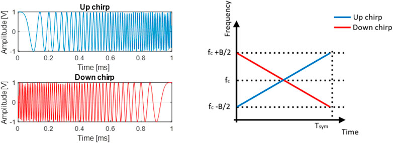
FIGURE 1. The up chirp and the down chirp in time domain (left) and frequency domain (right).
The CSS modulation order is defined as
The bandwidth
The CSS technique allows the symbol generation based on the
where
2.2 Direct Sequence Spread Spectrum (DSSS)
DSSS technology is a wideband modulation in which the original bit sequence is converted into a pseudo-random spreading sequence (Yue et al., 2003; Tsai, 2009). The direct-sequence modulation makes the transmitted signal wider in bandwidth than the information bandwidth. The pseudo-random code is modulated onto the information signal using several modulation techniques such as binary phase-shift keying (BPSK), quadrature phase-shift keying (QPSK) and so on. A transmission DSSS signal using BPSK modulation can be written as:
where

FIGURE 2. DSSS transmitter block diagram.
DSSS significantly improves protection against interfering and jamming signals, especially narrowband and makes the signal less noticeable. In the DSSS systems, each user is assigned a unique code sequence that allows the user to spread the information signal across the assigned frequency band (Javed et al., 2020).
2.3 Frequency Hopping Spread Spectrum (FHSS)
FHSS is a transmission technology used in wireless networks to generate spread spectrum by hopping the carrier frequency in a pseudo-random manner (Liu et al., 2017; Lei et al., 2018). For example, in a FHSS system, the transmitted signal is spread across multiple channels, as shown in Figure 3. The full bandwidth is divided into 6 channels, centred at
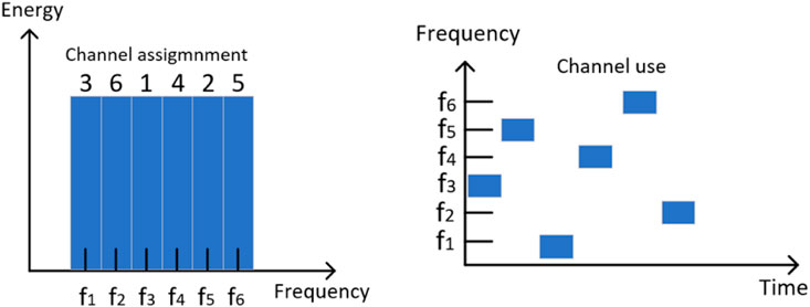
FIGURE 3. Channel assignment and channel use in FHSS.
Figure 4 shows the block diagram of a typical FHSS transmitter. First, digital data is modulated usually using some digital-to-analogue scheme. This baseband signal is then modulated onto a carrier
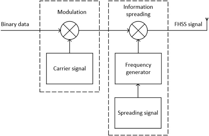
FIGURE 4. FHSS transmitter block diagram.
The transmitted FHSS signal can be expressed as:
where
Some of the advantages of using FHSS modulation are given by: improved privacy, avoiding interference and multi path fading, decreasing narrowband interference, increasing signal capacity, increasing the efficiency of bandwidth and the difficulty of interception. The transmission of a FHSS signal can share a frequency band with many types of conventional transmissions with minimal interference (Hong et al., 2013).
3 Classical approaches
In this section we detail two classic approaches used for modulation recognition that also provide the comparative support for the new proposed method based on the phase diagram analysis.
3.1 Wavelet transform approach
The wavelet transform is used to decompose a signal
where
As a result of this projection, we obtain a two-dimensional function called continuous wavelet transform. From here the scalogram, which renders the signal energy distribution for the scale
As a general remark on the use of this technique, one can say that the wavelet transform is able to quantify the time-frequency variations, but depends on the scale provided by the wavelet basis. That’s why in order to have a good wavelet representation, it is essential to determine the best suitable mother function which resembles as much as possible the analyzed transient signal.
3.2 Statistical approach
In the statistical approach are many sets of features that can be used in the signal recognition discrimination process. In this paper we use an approach based on the normalized central moments of the modulated signals. A central moment is a statistical moment that characterizes the probability distribution of a random variable with respect to its mean. The central moments are useful because they allow us to quantify properties of distributions in ways that are location-invariant, as in Eq. 12:
where
It is important to note that the central moments are valid only for distributions that have well-defined first and second moments, with the second moment being non-zero. Fortunately, this criterion applies to the majority of distributions. By standardizing the moments, they become invariant to both location and scale.
4 Phase diagram-based entropy approach
The phase diagram representation method is derived from the theory of nonlinear dynamical systems and it is a data–driven technique that makes no a priori assumption about the system (Zbilut and Webber, 1992; Davidson and Loughlin, 2000). Starting from a signal expressed as a time series, as in (13), the strategy for the phase diagram design is given by moving from the values of the signal to a new vector that defines the representation space as shown in Eq. 14:
where
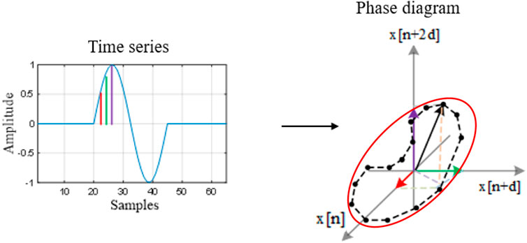
FIGURE 5. Example of a time series and its phase diagram representation.
This new resulting representation space can provide several ways of quantifying the information of the analyzed signal. One of the things of interest that can be quantified from the phase diagram is the distances between the phase diagram vectors because this establishes the shape of the trajectory. Based on this, we have the possibility to quantify the distribution of the phase diagram vectors (Stanescu et al., 2021). In the quantification process we use a probabilistic approach and we are interested in determining the probability of the signal to pass through a specific region of the phase diagram. Mathematically, we determine the number of points, which are close within a distance
where
where
Next, we determine the entropy information in the representation dimension of the phase diagram based on the number of total points, which satisfy the mentioned criterion, as described in Eq. 17.
It is interesting to see how the entropy information change form one dimension to another, that’s why we define the phase diagram-based entropy as a gradient of entropy from one dimension to another as in Eq. 18. This approach is used to study the behavior of the signal by measuring the changes that occur as an increase of the embedding dimension (Stanescu et al., 2021).
Thus, using this approach, we can successfully characterize the modulation signals in order to realize their recognition process. The advantages of the characterization of single carrier modulations based on the phase diagram approach were already shown in (Scripcaru et al., 2020; Stanescu et al., 2022; Stanescu et al., 2023). In order to address the characterization of different modulation, the sliding windows are used and the PDE is computed on each window.
5 Results
In this section we detail the results obtained in the characterization process of each type of modulation, then we discuss the accuracy of the recognition process by comparing our approach with other approaches used at the moment. The characterization of the signals will be done first in the noise-free scenario, after which the use of the approach in the presence of noise is studied.
5.1 CSS characterization
First, we analyze the CSS modulation. For this, we generate a CSS waveform, with the following parameters: the center frequency
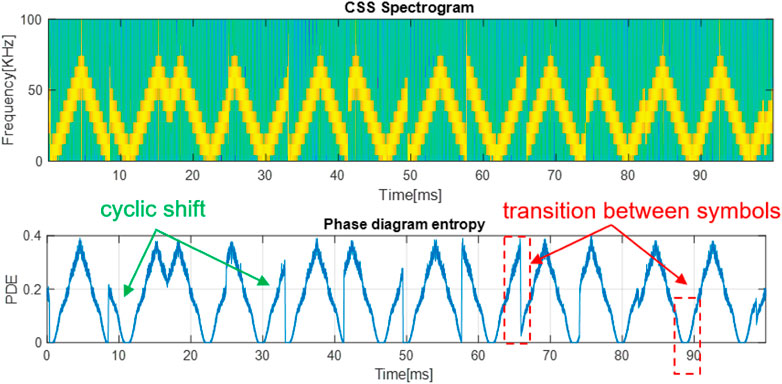
FIGURE 6. The CSS spectrogram and the PDE variation for
As shown, the PDE variation highlights the cyclic shift of each symbol. Moreover, the symbols are delimited by global minima and maxima values of the PDE and sudden entropy drops as it can be seen marked with the red dashed line. These proprieties are also present in the case of the signal with
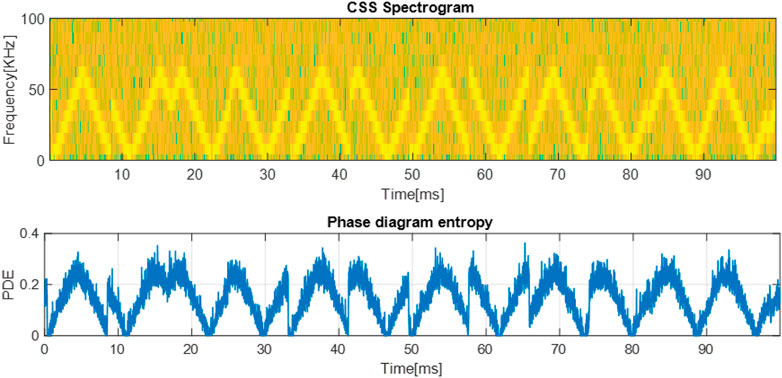
FIGURE 7. The CSS spectrogram and the PDE variation for
After showing the potential of the PDE for the characterization of the CSS signal, we want to see what the PDE variation distribution looks like. The phase diagram entropy distribution is shown in their corresponding histograms. In Figure 8, are displayed the histograms of the PDE of the CSS signal in the two cases.
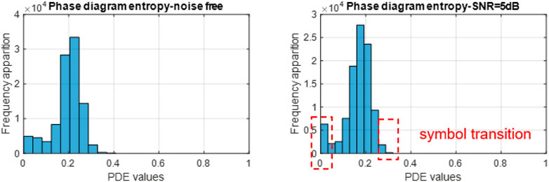
FIGURE 8. CSS signal phase diagram entropy histogram in the noise free case (left) and in the noisy case (right).
As we can see, the linear sweep of the signal quantified through the PDE values is grouped on the left side of the representation. We propose to quantify the transitions between CSS symbols based on the extremity bins of the histograms. Thus, we define the parameter Left Side Ratio (LSR) as the ratio between frequency of occurrence of the entropy values in extremity bins and frequency of occurrence of the remaining bins, as in Eq. 19:
where
5.2 DSSS characterization
In the analysis of the DSSS signal, we start from generating the 20 bits pattern with each bit, having a duration of
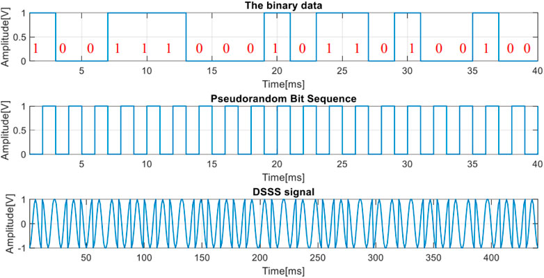
FIGURE 9. The data encoding signal (up), the pseudo-random sequence (middle) and the resulted DSSS signal.
In Figure 10 are displayed the DSSS signals and their PDE variation for the two cases. Each phase change of the DSSS signal leads to the appearance of a spike in the PDE variation. This is valid both in the noise free case and in the case of
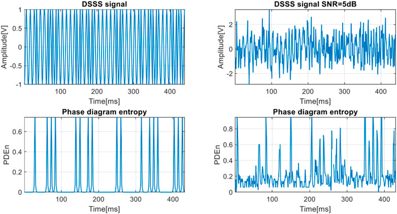
FIGURE 10. The DSSS signal and the phase diagram entropy variation for
In order to increase the characterization capacity of the DSSS modulation, we analyze the PDE variation distribution. The histograms of the DSSS signal are displayed in Figure 11.
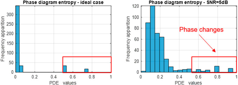
FIGURE 11. DSSS signal phase diagram entropy histogram in the noise free case (left) and in the noisy case (right).
We see that the transition between DSSS symbols, related to an increased value of PDE, is highlighted by the bins on the right side of the representation. In order to quantify this aspect, we define the Right-Side Proportion (RSP) as the ratio between the frequency of occurrence of the entropy values in the right half of the histogram representation and the total number of occurrences, as in Eq. 20:
where
5.3 FHSS characterization
In the analysis of the FHSS signal, we start from generating the 25 bits pattern with each bit, having a duration of
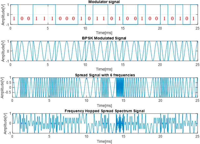
FIGURE 12. The data encoded signal, the BPSK modulated signal, the spread signal with 6 frequencies and the FHSS signal.
As can be seen in Figure 13, depending on the frequency of the signal we have a certain law of variation for the phase diagram entropy, each law being different from the other. Also, through the existence of more or less pronounced spikes, the transition from one frequency to another is captured. These observations are valid both in the noise free case and in the case of

FIGURE 13. The FHSS signal and the phase diagram entropy variation for
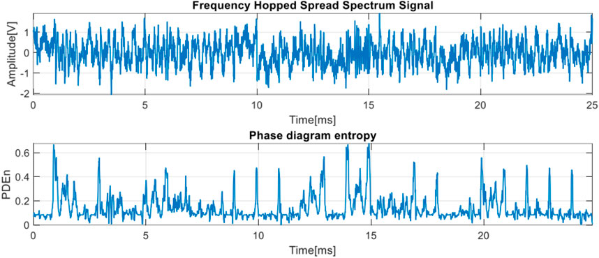
FIGURE 14. The FHSS signal and the phase diagram entropy variation for
In order to strengthen the recognition of the modulation with the help of the phase diagram entropy, we also use the histogram to be able to help us in the noisier cases. Analyzing the histograms in Figure 15, we can see the tendency of the frequency of occurrence to decrease, starting with the maximum bin based on an exponential law with a subunit basis.
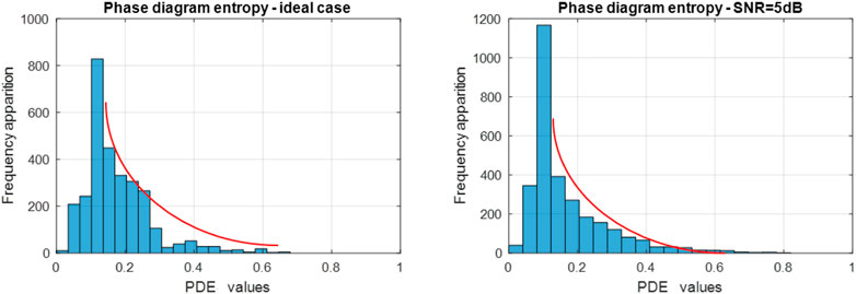
FIGURE 15. FHSS signal phase diagram entropy histogram in the noise free case (left) and in the noisy case (right).
Thus, we define the percentage of decreasing values (PDV) as the ratio between the frequency of occurrence of bins smaller than the bin with the most entropy values and the total number of values as in Eq. 21:
where
5.4 Modulation recognition accuracy
Based on the previous section, the approach that exploits the phase diagram-based entropy highlights unique characteristics for each type of spread spectrum modulation. Moreover, based on three statistical parameters derived from the PDE variation histograms, each modulation can be highlighted. Thus, Figure 16 presents the block diagram that we use to classify the spread spectrum modulations in totally blind conditions.
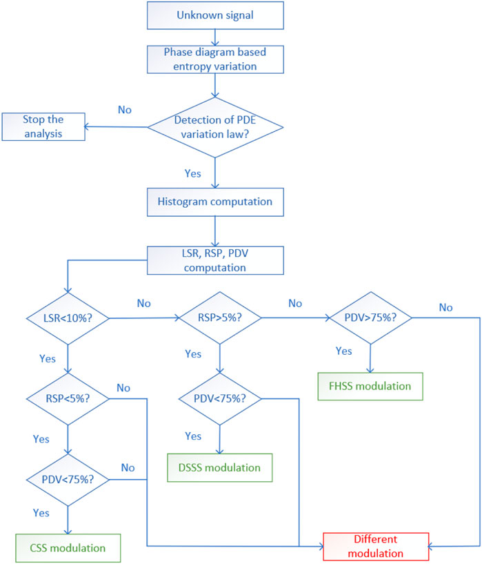
FIGURE 16. The block diagram for the classification of spread spectrum modulations.
In order to see the accuracy of the proposed approach, we will further see how the recognition algorithm behaves in the presence of noise. Thus, in Figure 17 we see the recognition accuracy for the three types of signals. The accuracy was calculated for a set of 100 synthetic signals from each type of modulation. In the process of determining the accuracy, we used the algorithm described in the block diagram, for each modulated signal, analyzing the variation of the three statistical parameters extracted from the PDE. This procedure was repeated for a wide range of SNRs to be able to see the behavior of the algorithms in low SNR cases.
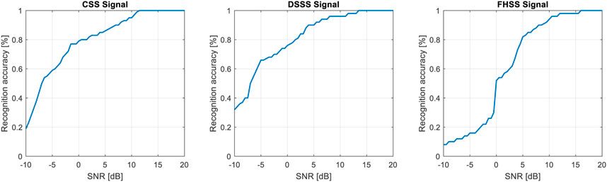
FIGURE 17. The recognition accuracy for the proposed approach for the spread spectrum signals.
The three graphs highlight a high accuracy for positive SNR values. For example, at
We turn our attention to some feature-based classic approaches for signal recognition in order to be able to compare the classical approaches with our proposal. We have as reference the spread spectrum signals for
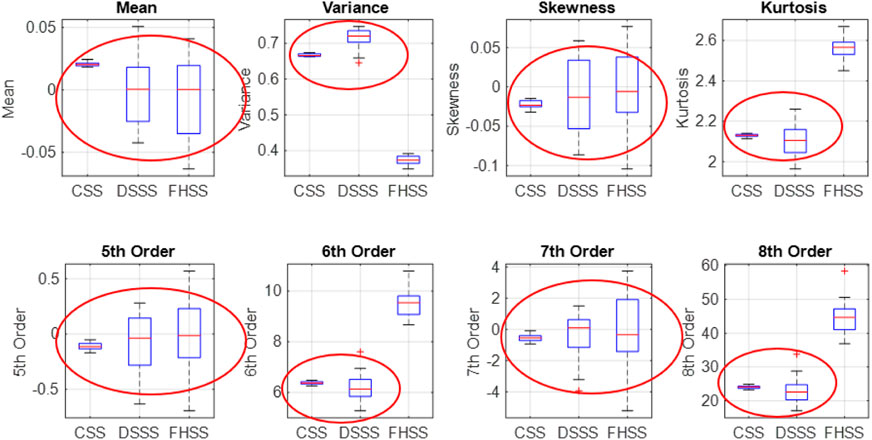
FIGURE 18. The first eight normalized central moments of the spread spectrum signals.
As can be seen, this approach does not present a desirable procedure to be used because the information provided is not sufficient to recognize the modulation. Most of the moments have identical values for the three types of signals and cannot offer even a possibility to recognize them. Also, the values of these parameters do not highlight anything specific for each signal.
Another approach used in modulation recognition is that given by the use of the wavelet transform (Li et al., 2019; Al-Makhlasawy et al., 2021). Figure 19 shows the scalograms of the three signals, in the determination of which a 10th order Daubechies wavelet generator is used.
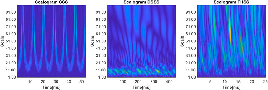
FIGURE 19. The scalograms of the three spread spectrum signals.
Analyzing the figure above, we notice that the analysis based on the wavelet transform has as a disadvantage the existence of a large number of representation scales and it is difficult to differentiate between scalograms based on these representations. One piece of information that we can quantify from these representations are the detection curves, shown in Figure 20.
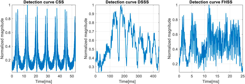
FIGURE 20. The detection curves using the scalograms of the three spread spectrum signals.
The detection curve of the CSS signal highlights the five pulses, but for the other two signals, the information provided is not relevant and does not highlight anything specific.
From the scalograms we can also extracts the detail coefficients at the coarsest scale from the wavelet decomposition (Park et al., 2008; Kumar et al., 2017) of the three signals. Figure 21 shows these coefficients for three levels of the signals.
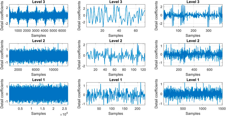
FIGURE 21. The detail coefficients for CSS signal (left), DSSS signal (middle) and FHSS signal (right).
The type of signal analyzed is too complicated to be characterized with these coefficients. Only the CSS signal shows some specific features in the detail coefficients of level 2 and 3, but the detail coefficients of the DSSS and FHSS signals cannot help in the recognition process of these modulations.
To highlight the capabilities of our approach, we use these two classic approaches as comparisons. The statistical approach uses the eight normalized central moments of the spread spectrum signals as features and the wavelet-based approach uses the three detail coefficients from the wavelet decomposition as features. Our approach consists in using the set consisting of the three statistical parameters derived from the PDE, namely, LSR, RSP and PDV as input for the ML classifiers. We use five Machine Learning classifiers: Support Vector Machine (SVM), Naïve Bayes (NB), k-Nearest Neighbors (kNN), Decision Tree (DT) and Quadratic Discriminant Analysis (QDA) in order to see which one is more appropriate for our classification process. The accuracy of the classification process is given by the confusion matrices obtained for the three sets of features. A visual representation of the input sets, the ML classifiers and the output is shown in Figure 22.
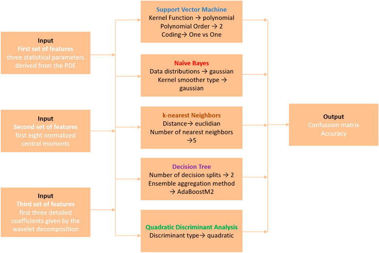
FIGURE 22. The illustration of the set of input features, the ML algorithms used and the output.
The classification result using the five ML classifiers is shown in Figure 23.
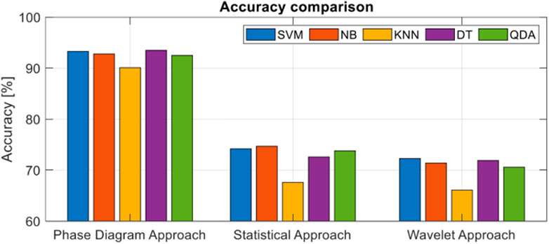
FIGURE 23. The classification accuracy using different approach and different classifiers.
The phase diagram-based approach offers the best results, with results over 90% depending on the classifier. The statistical approach provides poor results in terms of accuracy. Due to the fact that many of these moments are identical for the three classes of signals, the maximum accuracy we obtain is 74.7% using Naïve Bayes algorithm. The wavelet-based approach offers the worst results in the classification process of spread spectrum modulation. The maximum obtained for this approach is 72.3% using Support Vector Machine algorithm. The classical analysis methods, although they offer weaker results than the proposed method, have some advantages that can be used in certain contexts. For example, the statistical approach is simple to implement, it does not require the knowledge of additional information about the analyzed signal and the computational time related to this method is low. Also, the scalograms generated by the wavelet transform can be used with Deep Learning elements to increase the classification accuracy based on image classification algorithms.
From the perspective of ML algorithms, their functionality depends on the features used in the training process. Due to the particularities highlighted by the phase diagram entropy, DT offer a result of 93.5%, which is the highest, and kNN 90.2%, which is the lowest. The best results are obtained with DT because it is a non-parametric algorithm and it does not depend on probability distribution assumptions, working well on high-dimensional data. In addition, it uses a boosting algorithm to increase the performance. The worst results are obtained with kNN because kNN is a distance-based algorithm, this meaning that the cost of calculating the distance between a new point and each existing point is very high if we have a large dataset. That is why it does not work well with a high number of dimensions. In addition, kNN is a lazy algorithm and it does not have a training process in which the accuracy can be optimized.
6 Conclusion
Using the phase diagram entropy as a new alternative for the analysis of communication signals, we show the potential to extract important information about the analyzed signals and identify the type of modulations used, without prior knowledge. In this paper, we study the behavior in noisy backgrounds, of the parameters extracted from the spread spectrum signals using the phase diagram-based entropy and we propose some statistical parameters derived from the entropy distribution to recognize the signals. This approach proved to be very useful for the characterization and recognition of spread spectrum modulations being able to highlight defining characteristics for each type of modulation, which led to an accuracy higher than 90% in the classification process.
Three classes of spread spectrum modulations found in many commercial and military systems have been analyzed and characterized. The modulation recognition capability of the implemented algorithm is very high. Using this approach, we were able to highlight hidden features, invisible to other classical methods. We compared the proposed method with two feature-based classical methods based on high order statistical moments and wavelet transform. The results obtain using our approach exceed by more than 15% the results obtained using these classical approaches.
In our future work, we are planning to analyze a larger class of communication signals and study the capability of presented approach for higher orders of modulation. The robustness to the noise will be also addressed and we plan to refine our method to work at much lower SNR.
Data availability statement
The raw data supporting the conclusion of this article will be made available by the authors, without undue reservation.
Author contributions
Conceptualization, DS, AD, and CI; methodology, DS; software, DS; validation, AD, CI, and AS; formal analysis, DS; investigation, DS, AD; resources, DS; data curation, CI; writing—original draft preparation, DS; writing—review and editing, AD and CI; visualization, DS; supervision, AS; project administration, AD; funding acquisition, CI; All authors contributed to the article and approved the submitted version.
Funding
This work has been supported by ALTUS project funded by SATT Linksium. The author(s) declare financial support was received for the research, authorship, and/or publication of this article. This study is funded by SATT Linksium.
Conflict of interest
The author AS declared that they were an editorial board member of Frontiers, at the time of submission. This had no impact on the peer review process and the final decision.
The remaining authors declare that the research was conducted in the absence of any commercial or financial relationships that could be construed as a potential conflict of interest.
Publisher’s note
All claims expressed in this article are solely those of the authors and do not necessarily represent those of their affiliated organizations, or those of the publisher, the editors and the reviewers. Any product that may be evaluated in this article, or claim that may be made by its manufacturer, is not guaranteed or endorsed by the publisher.
References
Abu-Romoh, M., Aboutaleb, A., and Rezki, Z. (2018). Automatic modulation classification using moments and likelihood maximization. IEEE Commun. Lett. 22 (5), 938–941. doi:10.1109/LCOMM.2018.2806489
Al-Makhlasawy, R. M., Ghanem, H. S., Kassem, H. M., Elsabrouty, M., Hamed, H. F. A., Abd El-Samie, F. E., et al. (2021). Deep learning for wireless modulation classification based on discrete wavelet transform. Int. J. Commun. Syst. 34 (18). doi:10.1002/dac.4980
Davidson, K. L., and Loughlin, P. J. (2000). Instantaneous spectral moments. J. Frankl. Inst. 337 (4), 421–436. doi:10.1016/S0016-0032(00)00034-X
Dobre, O. A., Abdi, A., Bar-Ness, Y., and Su, W. (2007). Survey of automatic modulation classification techniques: Classical approaches and new trends. IET Commun. 1, 137. doi:10.1049/iet-com:20050176
Eckmann, J.-P., Kamphorst, S. O., and Ruelle, D. (1987). Recurrence plots of dynamical systems. Europhys. Lett. 4, 973–977. doi:10.1209/0295-5075/4/9/004
Gacanin, H. (2019). Autonomous wireless systems with artificial intelligence: A knowledge management perspective. IEEE Veh. Technol. Mag. 14, 51–59. doi:10.1109/MVT.2019.2920162
Gui, G., Sari, H., and Biglieri, E. (2019). A new definition of fairness for non-orthogonal multiple access. IEEE Commun. Lett. 23, 1267–1271. doi:10.1109/LCOMM.2019.2916398
Hong, S., Cheun, K., Lim, H., and Cho, S. (2013). Performance of M-ary turbo coded synchronous FHSS multiple access networks with noncoherent MFSK under Rayleigh fading channels. J. Commun. Netw. 15, 601–605. doi:10.1109/JCN.2013.000109
Huang, J., Zhou, Y., Sun, N., Hu, Z., and Kang, Y. f. (2010). “Cruciate ligament reconstruction using LARS artificial ligament under arthroscopy: 81 cases report,” in Proceedings of the 2010 International Conference on Communications and Intelligence Information Security, Xi'an, China, October 2010, 160–164. doi:10.1109/ICCIIS.2010.39123
Iglesias, V., Grajal, J., Royer, P., Sanchez, M. A., Lopez-Vallejo, M., and Yeste-ojeda, O. A. (2015). Real-time low-complexity automatic modulation classifier for pulsed radar signals. IEEE Trans. Aerosp. Electron. Syst. 51, 108–126. doi:10.1109/TAES.2014.130183
Javed, H., Khalid, M. R., and Soomro, H. (2020). “A novel practical method for blind detection of DSSS signal in multiple signals environment,” in Proceedings of the 2020 17th International Bhurban Conference on Applied Sciences and Technology (IBCAST), Islamabad, Pakistan, January 2020, 664–668. doi:10.1109/IBCAST47879.2020.9044593
Karapistoli, E., Pavlidou, F.-N., Gragopoulos, I., and Tsetsinas, I. (2010). An overview of the IEEE 802.15.4a Standard. IEEE Commun. Mag. 48, 47–53. doi:10.1109/MCOM.2010.5394030
Khan, M. T., Sha’ameri, A. Z., Zabidi, M. M. A., and Chia, C. C. (2022). “FHSS signals classification by linear discriminant in a multi-signal environment,” in Proceedings of the International e-Conference on Intelligent Systems and Signal Processing, Singapore, June 2022. Editors F. Thakkar, G. Saha, C. Shahnaz, and Y.-C. Hu, 143–155. doi:10.1007/978-981-16-2123-9_111370
Kumar, S., Bohara, V. A., and Darak, S. J. (2017). “Automatic modulation classification by exploiting cyclostationary features in wavelet domain,” in Proceedings of the 2017 Twenty-Third National Conference on Communications (NCC), Chennai, India, March 2017, 1–6. doi:10.1109/NCC.2017.8077145
Lee, J., An, J., Ra, H., and Kim, K. (2020). Long-range acoustic communication using differential chirp spread spectrum. Appl. Sci. 10 (24), 8835. doi:10.3390/app10248835
Lei, Z., Yang, P., and Zheng, L. (2018). Detection and frequency estimation of frequency hopping spread spectrum signals based on channelized modulated wideband converters. Electronics 7, 170. doi:10.3390/electronics7090170
Li, W., Dou, Z., Qi, L., and Shi, C. (2019). Wavelet transform based modulation classification for 5G and UAV communication in multipath fading channel. Phys. Commun. 34, 272–282. doi:10.1016/j.phycom.2018.12.019
Liu, W., Huang, K., Zhou, X., and Durrani, S. (2017). Full-duplex backscatter interference networks based on time-hopping spread spectrum. IEEE Trans. Wirel. Commun. 16, 4361–4377. doi:10.1109/TWC.2017.2697864
Madhavan, N., Vinod, A. P., Madhukumar, A. S., and Krishna, A. K. (2013). Spectrum sensing and modulation classification for cognitive radios using cumulants based on fractional lower order statistics. AEU - Int. J. Electron. Commun. 67 (6), 479–490. doi:10.1016/j.aeue.2012.11.004
Mallat, S. G. (2009). A wavelet tour of signal processing: The sparse way. 3rd. Amsterdam; Boston: Elsevier/Academic Press.
Marwan, N., Carmenromano, M., Thiel, M., and Kurths, J. (2007). Recurrence plots for the analysis of complex systems. Phys. Rep. 438, 237–329. doi:10.1016/j.physrep.2006.11.001
Park, C.-S., Choi, J.-H., Nah, S.-P., Jang, W., and Kim, D. Y. (2008). “Automatic modulation recognition of digital signals using wavelet features and SVM,” in Proceedings of the 2008 10th International Conference on Advanced Communication Technology, Gangwon, Korea (South), February 2008, 387–390. doi:10.1109/ICACT.2008.4493784
Qian, Y., Ma, L., and Liang, X. (2018). Symmetry chirp spread spectrum modulation used in LEO satellite internet of things. IEEE Commun. Lett. 22, 2230–2233. doi:10.1109/LCOMM.2018.2866820
Ravi Kishore, T., and Rao, K. D. (2017). Automatic intrapulse modulation classification of advanced LPI radar waveforms. IEEE Trans. Aerosp. Electron. Syst. 53, 901–914. doi:10.1109/TAES.2017.2667142
Raza, U., Kulkarni, P., and Sooriyabandara, M. (2017). Low power wide area networks: An overview. IEEE Commun. Surv. Tutorials 19, 855–873. doi:10.1109/COMST.2017.2652320
Reynders, B., and Pollin, S. (2016). “Chirp spread spectrum as a modulation technique for long range communication,” in Proceedings of the 2016 Symposium on Communications and Vehicular Technologies (SCVT), Mons, Belgium, November 2016, 1–5. doi:10.1109/SCVT.2016.7797659
Scripcaru, R., Nastasiu, D., Digulescu, A., Stanescu, D., Ioana, C., and Serbanescu, A. (2020). “On the potential of phase diagram analysis to identify the wide band modulations,” in Proceedings of the 2020 13th International Conference on Communications (COMM), Bucharest, Romania, June 2020, 55–58. doi:10.1109/COMM48946.2020.9141963
Stanescu, D., Digulescu, A., Ioana, C., and Serbanescu, A. (2021). “A novel approach for characterization of transient signals using the phase diagram features,” in Proceedings of the 2021 IEEE International Conference on Microwaves, Antennas, Communications and Electronic Systems (COMCAS), Tel Aviv, Israel, November 2021, 299–304. doi:10.1109/COMCAS52219.2021.9629068
Stanescu, D., Digulescu, A., Ioana, C., and Serbanescu, A. (2022). Modulation recognition of underwater acoustic communication signals based on phase diagram entropy. OCEANS 2022, 1–7. doi:10.1109/OCEANS47191.2022.9977145
Stanescu, D., Nastasiu, D., Ioana, C., and Digulescu, A. (2023). Characterization of digital modulations using the phase diagram analysis. Eur. Phys. J. Special Top. 232 (1), 187–199. doi:10.1140/epjs/s11734-022-00744-x
Tsai, Y.-R. (2009). M-ary spreading-code-phase-shift-keying modulation for DSSS multiple access systems. IEEE Trans. Commun. 57, 3220–3224. doi:10.1109/TCOMM.2009.11.050526
Wang, Xiaowei, Fei, Minrui, and Li, Xin (2008). “Performance of chirp spread spectrum in wireless communication systems,” in Proceedings of the 2008 11th IEEE Singapore International Conference on Communication Systems, Guangzhou, China, November 2008, 466–469. doi:10.1109/ICCS.2008.4737227
Webber, C. L., and Zbilut, J. P. (1994). Dynamical assessment of physiological systems and states using recurrence plot strategies. J. Appl. Physiology 76, 965–973. doi:10.1152/jappl.1994.76.2.965
Wu, Hsiao-Chun, Saquib, M., and Yun, Zhifeng (2008). Novel automatic modulation classification using cumulant features for communications via multipath channels. IEEE Trans. Wirel. Commun. 7, 3098–3105. doi:10.1109/TWC.2008.070015
Xiao-Ming, Z., and Zhong-Zhao, Z. (2006). “Parameter estimation of DSSS signals with modified fourth-order cumulants,” in Proceedings of the First International Conference on Innovative Computing, Information and Control - Volume I (ICICIC’06), Beijing, China, August 2006, 126–129. doi:10.1109/ICICIC.2006.1331
Yang, Y., Chang, J.-N., Liu, J.-C., and Liu, C.-H. (2004). Maximum log-likelihood function-based QAM signal classification over fading channels. Wirel. Personal. Commun. 28, 77–94. doi:10.1023/B:WIRE.0000015422.23663.98
Yu, X., Li, L., Yin, J., Shao, M., and Han, X. (2019). “Modulation pattern recognition of non-cooperative underwater acoustic communication signals based on LSTM network,” in Proceedings of the 2019 IEEE International Conference on Signal, Information and Data Processing (ICSIDP), Chongqing, China, December 2019, 1–5. doi:10.1109/ICSIDP47821.2019.9173133
Yue, Guangrong, Ge, Lijia, and Li, Shaoqian (2003). “Analysis of ultra wideband signal interference to DSSS receiver,” in Proceedings of the 2003 4th IEEE Workshop on Signal Processing Advances in Wireless Communications - SPAWC 2003, Rome, Italy, June 2003, 229–233. doi:10.1109/SPAWC.2003.1318956
Keywords: spread spectrum, phase diagram-based entropy, modulation classification, modulation recognition, cognitive radio, electronic warfare
Citation: Stanescu D, Digulescu A, Ioana C and Serbanescu A (2023) Spread spectrum modulation recognition based on phase diagram entropy. Front. Sig. Proc. 3:1197619. doi: 10.3389/frsip.2023.1197619
Received: 31 March 2023; Accepted: 19 June 2023;
Published: 05 July 2023.
Edited by:
Lihua Yang, Sun Yat-sen University, ChinaReviewed by:
Edson Stevens Galagarza, Technological University of Panama, PanamaTahmid Al-Mumit Quazi, University of KwaZulu-Natal, South Africa
Copyright © 2023 Stanescu, Digulescu, Ioana and Serbanescu. This is an open-access article distributed under the terms of the Creative Commons Attribution License (CC BY). The use, distribution or reproduction in other forums is permitted, provided the original author(s) and the copyright owner(s) are credited and that the original publication in this journal is cited, in accordance with accepted academic practice. No use, distribution or reproduction is permitted which does not comply with these terms.
*Correspondence: Denis Stanescu, ZGVuaXMuc3RhbmVzY3VAbXRhLmNvbQ==; Angela Digulescu, YW5nZWxhLmRpZ3VsZXNjdUBtdGEucm8=