Automated segmentation and labeling of subcutaneous mouse implants at 14.1T

Magnetic resonance imaging (MRI) is a valuable tool for studying subcutaneous implants in rodents, providing non-invasive insight into biomaterial conformability and longitudinal characterization. However, considerable variability in existing image analysis techniques, manual segmentation and labeling, as well as the lack of reference atlases as opposed to brain imaging, all render the manual implant segmentation task tedious and extremely time-consuming. To this end, the development of automated and robust segmentation pipelines is a necessary addition to the tools available in rodent imaging research. In this work, we presented and compared commonly used image processing contrast-based segmentation approaches—namely, Canny edge detection, Otsu’s single and multi-threshold methods, and a combination of the latter with morphological operators—with more recently introduced convolutional neural network (CNN-) based models, such as the U-Net and nnU-Net (“no-new-net”). These fully automated end-to-end state-of-the-art neural architectures have shown great promise in online segmentation challenges. We adapted them to the implant segmentation task in mice MRI, with both 2D and 3D implementations. Our results demonstrated the superiority of the 3D nnU-Net model, which is able to robustly segment the implants with an average Dice accuracy of 0.915, and an acceptable absolute volume prediction error of 5.74%. Additionally, we provide researchers in the field with an automated segmentation pipeline in Python, leveraging these CNN-based implementations, and allowing to drastically reduce the manual labeling time from approximately 90 min to less than 5 min (292.959 s ± 6.49 s, N = 30 predictions). The latter addresses the bottleneck of constrained animal experimental time in pre-clinical rodent research.

1 Introduction

Small animals such as mice are often used in the pre-clinical setting to advance the understanding of implantation techniques and bio-compatibility properties of injected biomaterials, with the ultimate goal of translating these research outcomes into human clinical applications. To this aim, magnetic resonance imaging (MRI) has been widely used as a non-invasive imaging modality, with the availability of excellent imaging contrasts for soft tissues, enabling a wide range of applications, notably in drug development (Matthews et al., 2013). However, tissue segmentation in the pre-clinical setting in mice has so far mainly been carried out in the brain (Mulder et al., 2017; Gordon et al., 2018; De Feo et al., 2021). Often, the latter relies on the usage of a high-resolution brain atlas [e.g., Waxholm space atlas (Papp et al., 2014), or more recently, the SIGMA rat brain atlases (Barrière et al., 2019); see Johnson et al. (2021) for a comprehensive list of rat brain atlases], to which the acquired images are registered using a library of analysis tools such as FSL (Smith et al., 2004; Jenkinson et al., 2012). Often, the main objective in these studies is to obtain an accurate segmentation of different rat brain anatomical structures, so that anatomical properties such as volumes of different brain regions can then be assessed and compared between animal populations. Atlases differ between in vivo and ex vivo studies, with widely varying tissue contrast and spatial resolution (Johnson et al., 2021). For these reasons, it is often challenging to create robust automated segmentation pipelines for different brain tissues. To tackle these limitations, multi-atlas strategies to improve segmentation accuracy have been proposed (Bai et al., 2012; Ma et al., 2014), as well as the use of other imaging sequences such as diffusion-weighted imaging (DWI), which was shown to be useful in better defining anatomic boundaries in several rat brain atlases (Calabrese et al., 2014; Papp et al., 2014).

However, deep neural networks (DNNs), and in particular, the subset of convolutional neural networks (CNNs), have demonstrated superior segmentation outcomes compared to classical registration algorithms or multi-atlas methods (De Feo et al., 2021). CNNs can be trained to significantly outperform state-of-the-art registration-based methods, both in terms of higher segmentation accuracy and lower inference time. In small animal MRI studies, however, the use of CNNs was limited to skull-stripping (Roy et al., 2018) and brain tissue segmentation (De Feo et al., 2021) approaches. Therefore, when biomaterials are injected into different body parts of the animal, the resulting shapes of the injected volume need to be estimated, and no corresponding atlas can be found or created. Similarly to the brain, tissues around the injection site need to be robustly delineated. For instance, in Hillel et al. (2012), authors have used MRI for volumetric analysis of 4 different injected soft tissue fillers in 5 rats, but have not required extensive tissue segmentation techniques due to the small sizes of fillers and the use of porcine collagen for injections, which possesses good intensity differentiation properties from adjacent tissues. In Fischer et al. (2015), 24 rats were injected with silicone implants, but only a small subset (2 rats from each study group) underwent MRI volumetric implant characterization, and measurements were approximated as elliptic shapes, and performed by two blinded observers. However, segmentation by hand is often tedious, extremely time consuming, and prone to variability if different researchers annotate the data. Liu et al. (2016) studied different hydrogels’ morphologies injected in rats, but used a commercially available software suite (MIMICS 16.0) designed for human medical image analysis and segmentation to perform the 3D reconstructions of rat implants. While the latter may provide a satisfying workaround for certain applications, it is not readily available to a wider range of researchers working with rodents. Quintero Sierra et al. (2022) further analyzed properties of 3 different subcutaneously injected acellular membranes in 30 rats, and had to perform tedious pixel-by-pixel manual volume segmentation in all animals. More recently, Tawagi et al. (2023) studied different hydrogel discs injected dorsally in 8 rats, using in-house threshold-based MATLAB scripts for implant segmentation. Authors reported the poor contrast between unlabeled implants and surrounding tissue, and again had to resort to manual segmentation across all slices.

In this context, novel automated and robust segmentation pipelines are required to extract the volumes of the injected implants in a reasonable amount of time. Here, we investigate several implant segmentation methods based on algorithms derived from classical image processing approaches, such as edge detection (Canny), Otsu’s methods, and the combination of such threshold-based approaches with morphological operators. We then propose an adapted CNN-based U-Net model suitable for injected implants in small animals, and compare the performance of all methods for accurate volume prediction.

2 Materials and methods

2.1 Mice implantation

Implantation experiments were approved by the local Animal Care and Use Committee of the Canton of Vaud (Switzerland, authorization VD3063.1). Adult, female CD1 mice between 12 and 20 weeks old were purchased from Charles River Laboratories (Bar Harbor, Maine, United States) and hosted at the university facilities (CIBM, EPFL, Lausanne, Switzerland) with a 12 h light/dark cycle, a normal diet ad libitum, in a room with a controlled temperature of 22°C ± 2°C. All animals were left to acclimatize in the facility for at least 1 week before implantation. The back of anesthetized mice (4% and 2% isoflurane for induction and maintenance, respectively) was shaved and disinfected with Betadine (Mundipharma Medical Company, Germany). The biomaterial (Béduer et al., 2021) was injected into the subcutaneous space of the left lower back of the mice (400 μL per mouse) through a 20G catheter (Terumo Corp., Japan). The implantation outcome is illustrated in Figure 1.

FIGURE 1

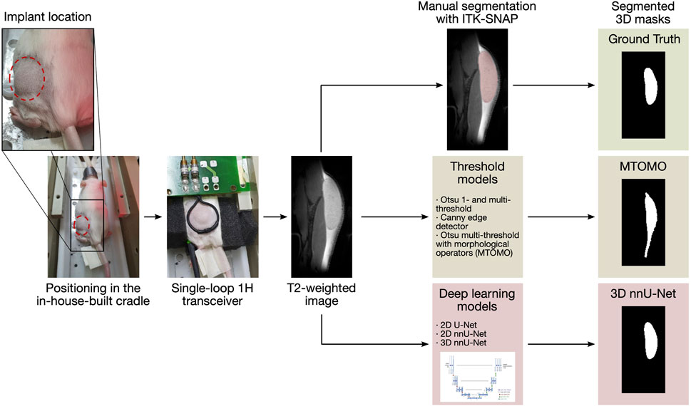
FIGURE 1. Illustration of the automated segmentation pipeline. The animal, with the implant injected in the lower back, is positioned in an in-house-built cradle and scanned. 144 T2-weighted slices are then available for segmentation. Time-consuming manual segmentation serves as reference (ground truth mask). Threshold models and CNNs are then evaluated and compared for the automated segmentation procedure.

2.2 MRI acquisition

All MRI experiments were performed on a 14.1 Tesla MRI system (Magnex Scientific, Oxford, United Kingdom) interfaced to a Bruker console (Paravision PV 360 v1.1, Ettlingen, Germany) located at the CIBM Centre for Biomedical Imaging (CIBM, Lausanne, Switzerland) and equipped with 1,000 mT/m gradients using an in-house-built 14 mm diameter single loop surface 1H transceiver placed on top of the injection site. During all MRI recordings, mice were placed in an in-house-built cradle, anesthetized with 1.5%–2% isoflurane in a 1:1 mixture of O2 and air (Figure 1). Body temperature and respiration rate were monitored using a small animal monitor system (SA Instruments, New York, United States). In addition, body temperature was maintained at 37°C using warm circulating water and was measured with a rectal temperature sensor. T2-weighted images were acquired on the lower back of 15 mice in which the biomaterial was injected using a TurboRARE sequence (RARE factor 2, TR = 2,000 ms, TE = 14 ms and 21 ms, field of view = 25 × 15 mm², 46 slices with 0.5 mm slice thickness, and 192 × 96 matrix size, with a resolution of 0.7 × 0.13 × 0.16 mm³) combined with a respiratory trigger. A total of 144 slices per image were then available for manual annotation.

2.3 Manual segmentation

After acquisition, anatomical MR images were segmented by hand using the ITK-SNAP software version 3.6.0 (Yushkevich et al., 2006). Slice-by-slice annotations were performed manually by defining the area of biomaterial implant using the polygon tool on top of each implant slice. 3D volumes were then reconstructed and quantified for each acquisition (Figure 2). These manually measured volumes were thereafter used as ground truth data for automated segmentation algorithms, in the form of binary masks with voxels encoded as 1 for implant and as 0 for background.

FIGURE 2

FIGURE 2. Reconstruction of manually labeled implants (manual segmentation) for 3 different mice (97-779G, 94-793G, and 92-778G). These examples illustrate the complexity, non-uniformity, and 3D variability of the implanted biomaterial.

2.4 CNN-based segmentation

Deep learning approaches are known for their excellent performance in segmentation tasks, in particular with U-Net architectures. U-Net is an image segmentation technique developed primarily for medical image analysis that can precisely segment images using a small amount of training data (Ronneberger et al., 2015). The U-Net architecture consists of a contracting path (encoder) and of an expanding path (decoder). The encoder extracts features at different levels through a sequence of convolutions, rectified linear unit (ReLU) activations, and max poolings, to capture the contents of each pixel. The number of feature channels is doubled at every down-sampling step, and the dimensions are reduced. The encoder learns to transform the input image into its features representation. The decoder is a symmetric expanding path that up-samples the result to increase the resolution of the detected features. The expanding path consists of a sequence of up-convolutions and concatenations with the corresponding feature map from the contracting path, followed by ReLU activations. The resulting network is almost symmetrical, with a U-like shape. Furthermore, in the U-Net architecture, skip-connections are added to skip features from the contracting path to the expanding path to recover spatial information lost during down-sampling. The presence of these additional paths has been shown to benefit model convergence (Drozdzal et al., 2016). To obtain the prediction on an input image, the model’s output is passed through a sigmoid activation function, which attributes to each pixel a probability reflecting its classification as implant or background. A threshold at p = 0.5 is then applied to round the pixel as either 1 or 0.

The architecture of the U-Net can be modified to become a 3D U-Net capable of segmenting 3-dimensional images. The core structure with contracting and expanding paths is kept, however, all 2D operators are replaced with corresponding 3D operators (3D convolutions, 3D max pooling, and 3D up-convolutions). Here, we implemented several U-Net models and compared classification performance metrics with respect to other non CNN-based models on the mice implant segmentation task. Namely, we trained a 2D U-Net model (Section 2.4.1), and 2D and 3D adaptations of a self-configuring model called nnU-Net (Section 2.4.2).

2.4.1 2D U-Net

The original U-Net architecture (designed for inputs of size 572 × 572 × 3 channels) was adapted in order to fit the segmentation task. Each MR input image was sliced according to its first dimension, yielding 46 slices of 192 × 96 × 3 channels. The output was modified to yield a single channel, in accordance to the pixel-wise binary classification problem. Padding was matched for same vector size to avoid shrinkage during convolutions, and batch normalization was added after each ReLu activation to accelerate the training. A total of 15 million trainable parameters was kept. The weights of the model were initialized randomly, and the batch size was set to 5 slices. Each slice was normalized, and both the mean and standard deviation were fixed. The BCEWithLogitsLoss loss function from PyTorch was selected to better deal with the unbalanced data set (97.1% of pixels were labeled as background across all available slices). The loss was therefore defined as

$L\left(\mathbf{x},\mathbf{y}\right)=-\frac{1}{N|I|}\sum _{n=1}^N\sum _{i\in I}\left[p_c{y}_{n,i}\log \sigma \left(x_{n,i}\right)+\left(1-y_{n,i}\right)\log \left(1-\sigma \left(x_{n,i}\right)\right)\right](1)$

with N the number of slices in a given batch, |I| the number of pixels, y_n,i the true binary value (0 or 1) of pixel i in image n, and x_n,i the prediction for pixel i in image n. The weight of the positive answer p_c (for class c) was set to 10, after testing weights in the range (0, 20). As rare classes could end up being ignored because of under-representation during training, the weight of the positive answer was used to limit false negatives (i.e., predicting background instead of implant for a given pixel i in image n). The loss combines a sigmoid layer and the binary cross entropy loss (BCELoss) in one single class, and is more stable numerically (log-sum-exp trick). The stochastic gradient descent was replaced with the Adam optimizer (Kingma and Ba, 2017), known to converge faster during training. The learning rate was initially set to 0.1 and was multiplied by 0.8 every 50 epochs. These values were tuned through a grid search, maximizing the Dice coefficient on the validation set (see Section 3.2). The training was done for 250 epochs, and the model parameters were saved every 25 epochs. The evolution of the Dice coefficient on the train set stabilized after 100 epochs, and decreased on the validation set after 100 epochs. To avoid over-fitting, the model used for testing was trained with 100 epochs.

2.4.2 2D nnU-Net and 3D nnU-Net

nnU-Net is a robust and self-adapting framework based on 2D and 3D vanilla U-Nets (Isensee et al., 2021). It is a deep learning-based segmentation method that automatically configures itself. Three types of parameters are to be determined: fixed, rule-based, and empirical. Fixed parameters such as architecture design decisions or the training scheme are predetermined. Rule-based parameters are configured according to the data fingerprint (low dimensional representation of the data set properties), including dynamic network adaptation (input dimension), target spacing, and re-sampling of intensity normalization. Empirical parameters were determined by monitoring the performance on the validation set after training. The architecture is similar to the U-Net. It contains plain convolutions, instance normalization, and leaky ReLu for the activation functions. Two computational blocks per resolution stage were used in both encoder and decoder (Figure 3). Down-sampling was done with stride convolutions (stride $>$ 1), and up-sampling with transposed convolutions. While the framework offers 3 separate configurations (2D U-Net, 3D full resolution U-Net, and 3D U-Net cascade), the cascade configuration was not used because it is only beneficial when the input data is larger than the 3D full resolution U-Net’s patch size, which was not the case here. The optimizer was a stochastic gradient descent with a high initial learning rate (0.01) and a considerable Nesterov momentum (0.99). The learning rate was reduced during the training using the “polyLR” schedule, which follows an almost linear decrease to 0. The loss terms were averaged and consisted of the Dice loss and a cross-entropy loss. The latter is well suited to address the class imbalance problem and provides stability during training. Several data augmentation techniques were applied during the training, namely, rotation and scaling, addition of Gaussian noise, Gaussian blur, change in brightness and contrast, and gamma augmentation and mirroring. The models were trained in a 5-fold cross-validation loop with a fixed length of 1,000 epochs for each configuration (five customized training and validation sets were created). During the training, the framework kept in memory the weights yielding the best Dice accuracy on the validation set. At inference, the framework aggregated the result of the 5-fold models.

FIGURE 3

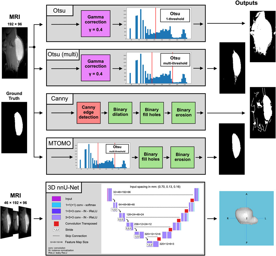
FIGURE 3. Block digrams for the compared threshold-based [Otsu one- and multi-threshold, Canny edge detector, and the combination of multi-threshold Otsu with morphological operators (MTOMO)] methods and for the best performing CNN-based 3D nnU-Net on the implant segmentation task, with illustrated 2D and 3D output examples, respectively.

2.5 Comparison with threshold models

Several other automated segmentation algorithms previously implemented in the laboratory and used for this data set were explored to compare classification performance with the deep learning-based automated segmentation implementations (2D U-Net, 2D and 3D nnU-Nets). These models, hereafter referred to as threshold models, included one- and multi-threshold Otsu methods, a Canny edge detection approach, and a combination of a multi-threshold Otsu method with additional morphological operations (MTOMO; Figure 3). These techniques were previously used in combination with manual segmentation, and made use of several contrast properties of the injected biomaterial (e.g., the average implant pixel was 82.5% brighter than its background surrounding tissue, and a convex and compact shape described most slices containing the implants).

The first thresholding algorithm is called Otsu (Otsu, 1979). It separates the pixels of an input image into several different classes according to the intensity of gray levels. For MR images, the brightest group was labeled as the implant and the other groups as the background. The Otsu single-threshold method was tested beforehand, but better results were observed when using multiple thresholds. To emphasize the differences in the images, a gamma correction technique was additionally applied. It is used to improve the brightness of the image and enhances the image contrast. Gamma correction is defined by the following power-law expression

$V_{\text{out}}=A{V}_{\text{in}}^{\gamma }(2)$

with V_in the input pixel value of the image, A a constant that was set to 1 and γ a parameter to fine-tune. Darker regions can be made lighter by using a γ smaller than 1. Several γ values were tested, and 0.4 was retained. Changing the intensity’s distribution allowed to enhance and highlight the image information.

To take into account the desired morphological shape, an edge detection algorithm was implemented. Edge detection is the detection of objects’ boundaries within an image, by means of intensities’ discontinuities analysis. This technique was used because the implant appears brighter than its surrounding tissue under to used MR contrast. The Canny edge detection method (Canny, 1986) was used, as it is known to provide the best results with strong edges compared to the other edge detection methods (Othman et al., 2009; Katiyar and Arun, 2014). The Canny edge detector is a multi-stage algorithm that uses the first derivative of a Gaussian to detect an edge in an image. It consists of five separate steps: noise reduction (smoothing), gradient seeking, non-maximum suppression, double threshold, and edge tracking by hysteresis. Finally, morphological operators were used to achieve better results, such as filling holes (binary closing) and reducing the shape of the detected implant (binary erosion). The different methods are illustrated in Figure 3 and are detailed in the Jupyter notebook semi-automatic-methods.ipynb (see Data Availability Statement).

2.6 Validation

The Dice similarity coefficient was used to quantify the accuracy of prediction for each model. The latter measures the similarity between two sets of data, and ranges from 0, indicating no spatial overlap between the two sets of binary segmentation results, to 1, indicating a complete overlap. It is defined as

$\mathrm{D}\mathrm{i}\mathrm{c}\mathrm{e}\left(A,B\right)=\frac{2\times |A\cap B|}{|A|+|B|}(3)$

with A being the set of predicted implant pixels and B the set of actual (ground truth) implant pixels. Additionally, every model presented in this manuscript was trained and tested on the same data split. 114 MRIs were split into a training, validation, and testing sets, in the respective proportions of 53%, 14%, and 33%. The test set contained 38 MR images (1036 2D images). The data was carefully split to avoid bias, such that any repeated measures from the same animal (if any) were present in only one of these three sets.

To complement Dice similarity, and as primary goal of this automated implant segmentation pipeline, implant volume estimates were computed for each prediction. A relative volume difference was computed as

$\mathrm{\Delta }{\mathrm{V}\mathrm{o}\mathrm{l}}_{\text{rel}}=\left(\frac{{\mathrm{V}\mathrm{o}\mathrm{l}}_{\text{pred}}-{\mathrm{V}\mathrm{o}\mathrm{l}}_{\text{lab}}}{{\mathrm{V}\mathrm{o}\mathrm{l}}_{\text{lab}}}\right)\times 100(4)$

with ΔVol_rel in %, Vol_pred the predicted volume from the output binary mask from each model, and Vol_lab the computed volume from manually labeled segmentation (i.e., ground truth). Validation metrics were then assessed on average segmentation outcomes (implant mask outputs) and per slice.

3 Results

3.1 Threshold models

The threshold and edge detection algorithms, as previously described in Section 2.5, were applied on the test set. These algorithms mostly delineated the implant shape at central sagittal locations (e.g., slice 25 out of 46 in Figure 4) but did not perform well at implant edge slices (e.g., slices 13–17 or 31–35). Multi-threshold Otsu performed better than its single-threshold alternative, as expected, but included many noisy pixels from the background. Canny edge detection was not sufficient for this task, and tissue features from the spine of rodents were also captured (Figure 4). The best threshold model was obtained by applying additional morphological operators, namely, binary closing and binary erosion (see Section 2.5), to the multi-threshold Otsu model (i.e., MTOMO), but overestimation of the implant volume had still occurred because of poor implant/tissue contrast.

FIGURE 4

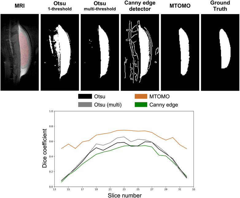
FIGURE 4. Illustration of threshold methods [Otsu one- and multi-threshold, Canny edge detector, and the combination of multi-threshold Otsu with morphological operators (MTOMO)] applied to a clean MRI slice (25 out of 46) of mouse 94-795G. The ground truth (last column) corresponds to the manual human segmentation. It is overlaid in a red shade onto the original MRI slice (left). All of the threshold models overestimated the implant volume at this location, with MTOMO yielding the best performance.

Because of the relatively poor performance of threshold-based models on this segmentation task, especially at implant edges, only the best performing model (MTOMO) was further selected for comparison with U-Net models.

3.2 Dice coefficients

For every model, average Dice coefficients were computed (as described in Section 2.6) across the test set. Results are summarized in Table 1, as averages with 95% confidence interval. As all implants are located within the slice range 10–35, the average Dice coefficients were computed per slice within the range 9–36 to exclude a significant amount of 2D images with background only. The 2D and 3D nnU-Nets were trained on the entire range of slices, but the 2D U-Net and the MTOMO model were trained on the subset of slices containing a part of an implant. However, comparisons were made separately to account for the number of slices. For comparison, the implants were further distinguished between their extremities (slices 11–17 and 29–34) and their average central part (slices 18–28). On average, the 3D nnU-Net model outperformed the other models with a Dice coefficient of 0.915 ± 0.011 (95% CI).

TABLE 1

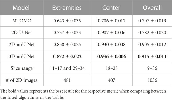
TABLE 1. Average Dice coefficients over the indicated slice ranges for the four compared models (multi-threshold Otsu with morphological operators (MTOMO), 2D U-Net, and 2D and 3D nnU-Nets), computed on a total of 1036 2D images in the test set. Confidence intervals at 95% are shown.

3.3 Volume estimates

The predicted volume was computed by counting the voxels classified as part of the implant within the output binary mask from each model, multiplied by the volume of a single voxel (i.e., 0.0146 mm³). Average (± standard deviation) differences were computed for each model across all predictions over the test set (Table 2). A negative average corresponds to volume underestimation, while a positive value reflects an average overestimation. The absolute average (|Average| in Table 2) was also computed to estimate the average absolute volume deviation from the manually labeled masks for each model. The latter accounts for volume under- and over-estimation across different predictions from the same model. The maximum error (Error_max in Table 2) represents the highest volume deviation obtained across all predictions for a given model. Additionally, the total training time (in hours) and prediction time (in seconds; for a given model to output a single binary 46 × 192 × 96 predicted implant mask) were estimated for each model.

TABLE 2

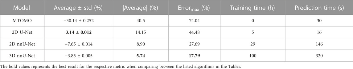
TABLE 2. Relative volume differences (ΔVol_rel, see Eq. 4), expressed as average (± standard deviation) and absolute average (|Average|), maximum prediction error (Error_max), and training and prediction times, for the four compared models (multi-threshold Otsu with morphological operators (MTOMO), 2D U-Net, and 2D and 3D nnU-Nets) on the test set.

While the best threshold model (MTOMO) highly underestimates the implant volume, only the 2D U-Net overestimates it. Both the 2D and 3D nnU-Nets underestimate the implant volume, but only by an absolute average error of 8.90% and 5.74%, respectively. The 3D nnU-Net therefore highly outperforms its 2D alternative, with a maximum error below 20% (17.79% in this test set). Even if the volume prediction errors are also reflected in the Dice coefficients (Table 1), a noticeable improvement can be seen for the 3D against the 2D nnU-Net. Indeed, while the different in Dice coefficients is low (0.915 against 0.905 on average, for all implant slices, Table 1), the 3D nnU-Net was substantially better at predicting a more accurate overall implant volume. Training times reflect models’ complexity, even if some were trained on GPUs rather than CPUs.

3.4 Comparison per slice

3.4.1 Dice coefficients per slice

The average Dice coefficient profile per slice for each model is shown in Figure 5. The resulting inverted U-shape across the four models illustrates the increased difficulty at correctly delineating the implant from the surrounding tissue at implant edge slices (e.g., see also Figures 8C, D), when poor contrast or non-convex shapes come into play. Hence, all four models exhibit increased prediction accuracy within the central slices 18–28, with 3D and 2D nnU-Nets performing the best. The performance drops associated with implant edges are due to numerous background pixels within extremity slices, as well as more atypical shapes previously unseen by the models. The 3D nnU-Net outperforms its 2D alternative by relying on previous slices at implant extremities, whereas each slice is processed independently in the 2D nnU-Net. This is further illustrated in Figure 6, in which the reconstructed predictions from both nnU-Net models show the added benefit of using the 3D version.

FIGURE 5

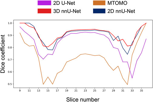
FIGURE 5. Comparison of the average Dice coefficient across implant-containing slices (9–36) for 4 different models (multi-threshold Otsu with morphological operators (MTOMO), simple 2D U-Net, and 2D and 3D nnU-Nets). On average, the 3D nnU-Net outperforms the other models in almost all slices. In particular, the 2D U-Net fails to properly capture the implant at edge locations (e.g., slices 32–36).

FIGURE 6

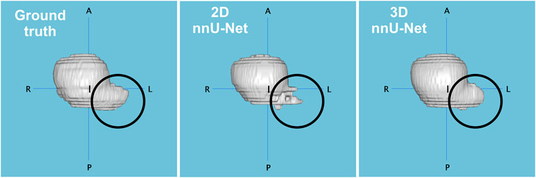
FIGURE 6. Comparison of reconstructions between the manual segmentation (ground truth), and the predictions of 2D and 3D nnU-Net models applied on the implant from one rodent (97-815G). Dice coefficients were 0.916 (2D) and 0.944 (3D), and predicted volume errors of 11.1% and 0.7%, respectively. The 3D nnU-Net model overcomes its 2D alternative by better capturing the implant structure at specific edge locations (circled).

3.4.2 Volume error per slice

Aside similar average Dice coefficients (Table 1), the 3D nnU-Net yielded better average volume predictions than its 2D alternative. This was also valid for the volume estimated per slice. Figure 7 shows the average and absolute average errors in number of pixels per slice for the two nnU-Net models. Dice coefficients per slice are also included.

FIGURE 7

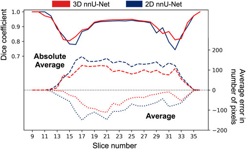
FIGURE 7. Average and absolute average errors in number of pixels for the 2D and 3D nnU-Net models. Average Dice coefficients are superimposed at the relevant slice locations. The 3D nnU-Net model performs better at several poor-contrast implant locations (e.g., slices 13–17, and 29–33), and shows a reduced average error over all slices. All implants were fully contained between slices 9–36.

On average, both models predicted a smaller number of pixels at every slice compared to the ground truth (negative dashed lines in Figure 7), which shows that volume under-estimation occurred at every slice. The absolute average curve shows once again that the 3D nnU-Net model performed better at central implant locations (slices 18–28) as compared to extremities (slices 11–17 and 29–34), at which the benefit of using the 3-dimensional model is less pronounced.

3.4.3 Segmentation outcomes

Models were further visually compared across different slices and rodents. Figure 8 illustrates 4 different segmentation outcomes across the 4 models. In (A), a central implant slice is shown, for which the 3D nnU-Net model achieved almost perfect segmentation (Dice coefficient of 0.988). This illustrates the benefit of automated segmentation at central implant locations. In (B), a more complex implant shape is shown. In this case, the 2D nnU-Net is unable to capture the smaller part of the implant because of its discontinuity. The 3D nnU-Net successfully captures the smaller part despite the introduced implant discontinuity. In (C), the 3D nnU-Net again outperforms the other models in a poor implant-tissue contrast slice. Finally, (D) illustrates the benefit of the 3D-trained model regarding the minimization of background pixels labeling as implant.

FIGURE 8

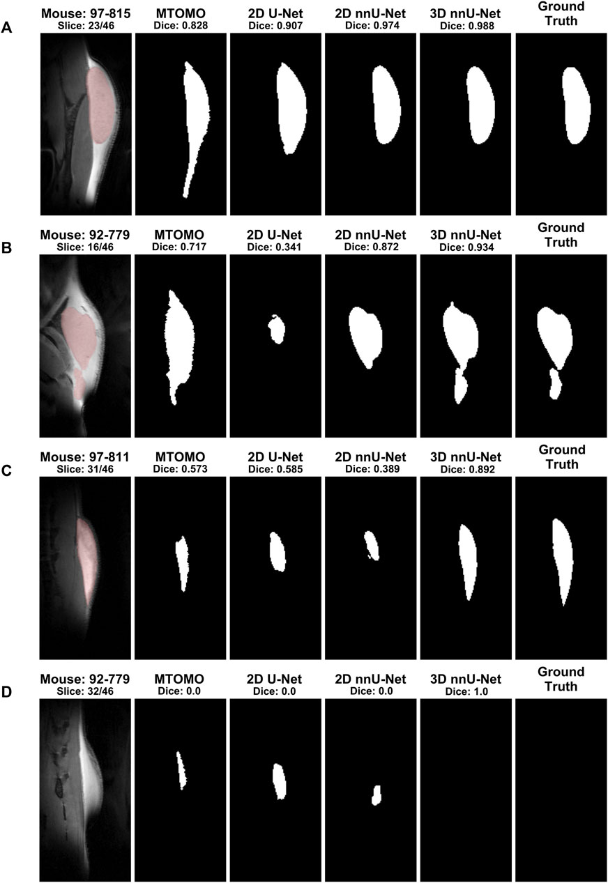
FIGURE 8. Examples of segmentation outcomes by different algorithms for selected slices. The ground truth column corresponds to manual segmentation, and its mask is overlaid (red shading) onto the MR image. (A) When the slice contains an easily identifiable implant shape, only the MTOMO model captures erroneous elongations due to similar tissue characteristics at the lower end of the implant. (B) For more complex implant shapes, the 3D nnU-Net is able to perform much better than the 2D alternatives, by capturing disjoint parts. (C) A similar effect can be seen for slices with poor implant versus tissue contrast. (D) At slices near the edge, the 3D nnU-Net correctly captures background tissue when no implant is present. These examples illustrate the robustness of the 3D nnU-Net model on this segmentation task.

4 Discussion

Our results demonstrate that CNN-based segmentation based on “no-new-nets” (nnU-Nets) can drastically improve classical threshold-based segmentation methods previously available for MR images, when no corresponding prior atlases (i.e., as for brain segmentation) are available. These results are in line with previous MRI-based segmentation literature in rodents (Holbrook et al., 2020; De Feo et al., 2021; Gao et al., 2021). However, to the best of our knowledge, this is the first contribution of a fully automated Python pipeline for non-brain implant segmentation in mice. Although the superiority of CNN-based segmentation models over more classical image processing approaches has already been shown in several medical imaging applications (Kayalibay et al., 2017), we here leveraged and compared CNN-based models, in particular the classical 2D U-Net (Ronneberger et al., 2015), as well as the more recently proposed nnU-Nets (Isensee et al., 2018; Isensee et al., 2021) in 2D and 3D, with so-far available threshold-based procedures. We have shown that the best performing threshold-based model, the multi-threshold Otsu combined with morphological operators (MTOMO), as well as the classical 2D U-Net architecture, were not robust enough to retain an acceptable segmentation accuracy, especially at implant edges. The nnU-Net architecture, especially in 3D, was more suitable to capture subtle implant characteristics in poor implant-tissue contrast conditions, as shown by the much higher average Dice coefficients obtained both at implant extremities and center. Moreover, the benefits of the 3D over the 2D implementation of the nnU-Net were substantial for the improved accuracy at implant edges, as well as for the minimization of background pixels’ classification as implant, as shown in several segmentation example outcomes. This improvement in accuracy can be attributed to the more sophisticated nnU-Net algorithm with a large number of trainable parameters, as compared to the classical image processing algorithms (Canny and Otsu) previously employed by researchers in the field.

Several limitations of the current models could be further addressed to improve these results. The recurrent average volume under-estimation by the 3D nnU-Net model, at the average and per slice levels, was certainly due to the class imbalance in the ground truth. This imbalance was addressed in the 2D U-net model by choosing an appropriate weight of the positive answer (for the under-represented implant class), yielding volume over-estimation, at the expense of decreased accuracy in volume prediction. Another limitation is that the implant shapes were relatively similar across mice, since the same amount of biomaterial was always injected, and because of the anatomy of the back of the mouse. Therefore, the model could be trained on more heterogeneous data, by estimating implants of lower or bigger size. However, published and available rodents’ implant data is scarce, which does not allow to further evaluate our pipeline on additional data sets. Here, the utilized data augmentation approaches for the nnU-Net models were not sufficiently modifying the shapes of the implants, making it more difficult for these models to deal with atypical and more complex shapes. Further research could include the implementation of different loss functions (Jadon, 2020; Ma et al., 2021), as the two metrics used here (Dice and volume estimates) only allow for a modest characterization of models’ performance. Moreover, interpretability of the trained model architecture could be further explored, as companion characterization tools begin to emerge (Alber et al., 2019). A bigger data sample, as well as improved MRI contrasts at 14.1 Tesla could further enhance these results. However, the primary goal of this manuscript was to present a novel segmentation pipeline for implants in rodents at high-field MRI, and to make it freely available to researchers in order to significantly decrease the time needed for manual segmentation and labeling, as well as to avoid costly software suites. Labeling by hand 46 slices (of 192 × 96 pixels) takes on average 90 min for an expert. In comparison, the 3D nnU-Net implementation proposed here achieves this task in 292.95 ± 6.49 s (N = 30 predictions), with an average accuracy (Dice coefficient) of 0.915 and an average absolute error of 5.74% on the predicted volume. In conclusion, the proposed automated segmentation pipeline may significantly ease the work of researchers working with rodents and MRI, still allowing for manual fine-tuning of small errors after automated CNN-based segmentation.

Data availability statement

The data analyzed in this study is subject to the following licenses/restrictions: The dataset is not available for public use. Requests to access these datasets should be directed to CC, cristina.cudalbu@epfl.ch.

Ethics statement

The animal study was approved by the Animal Care and Use Committee of the Canton of Vaud (Switzerland, authorization VD3063.1). The study was conducted in accordance with the local legislation and institutional requirements.

Author contributions

CC, NG, and MGP contributed to the conception and design of the study. GB performed animal experimentation and manual implant segmentation. JA performed all the analyses. JA, CC, and NG wrote the manuscript. All authors contributed to the article and approved the submitted version.

Funding

Animal experiments and imaging were performed thanks to InnoSuisse grants 38171.1 and 46216.1. MGP and CC were supported by the CIBM Center for Biomedical Imaging, a Swiss research center of excellence founded and supported by Lausanne University Hospital (CHUV), University of Lausanne (UNIL), Ecole Polytechnique Fédérale de Lausanne (EPFL), University of Geneva (UNIGE) and Geneva University Hospitals (HUG). Open access funding by École Polytechnique Fédérale de Lausanne.

Acknowledgments

The authors would like to thank Amélie Béduer for her help with the manuscript, and Anja Ðajić for her initial work with earlier segmentation approaches.

Conflict of interest

The authors declare that the research was conducted in the absence of any commercial or financial relationships that could be construed as a potential conflict of interest.

Publisher’s note

All claims expressed in this article are solely those of the authors and do not necessarily represent those of their affiliated organizations, or those of the publisher, the editors and the reviewers. Any product that may be evaluated in this article, or claim that may be made by its manufacturer, is not guaranteed or endorsed by the publisher.

References

Alber, M., Lapuschkin, S., Seegerer, P., Hägele, M., Schütt, K. T., Montavon, G., et al. (2019). iNNvestigate neural networks. J. Mach. Learn. Res. 20, 1–8. doi:10.48550/arXiv.1808.04260

CrossRef Full Text | Google Scholar

Bai, J., Trinh, T. L. H., Chuang, K.-H., and Qiu, A. (2012). Atlas-based automatic mouse brain image segmentation revisited: model complexity vs. image registration. Magn. Reson. Imaging 30, 789–798. doi:10.1016/j.mri.2012.02.010

PubMed Abstract | CrossRef Full Text | Google Scholar

Barrière, D., Magalhães, R., Novais, A., Marques, P., Selingue, E., Geffroy, F., et al. (2019). The SIGMA rat brain templates and atlases for multimodal MRI data analysis and visualization. Nat. Commun. 10, 5699. doi:10.1038/s41467-019-13575-7

PubMed Abstract | CrossRef Full Text | Google Scholar

Béduer, A., Bonini, F., Verheyen, C. A., Genta, M., Martins, M., Brefie-Guth, J., et al. (2021). An injectable meta-biomaterial: from design and simulation to in vivo shaping and tissue induction. Adv. Mater. 33, 2102350. doi:10.1002/adma.202102350

CrossRef Full Text | Google Scholar

Calabrese, E., Du, F., Garman, R. H., Johnson, G. A., Riccio, C., Tong, L. C., et al. (2014). Diffusion tensor imaging reveals white matter injury in a rat model of repetitive blast-induced traumatic brain injury. J. Neurotrauma 31, 938–950. doi:10.1089/neu.2013.3144

PubMed Abstract | CrossRef Full Text | Google Scholar

Canny, J. (1986). A computational approach to edge detection. IEEE Trans. pattern analysis Mach. Intell. 8, 679–698. doi:10.1109/tpami.1986.4767851

PubMed Abstract | CrossRef Full Text | Google Scholar

De Feo, R., Shatillo, A., Sierra, A., Valverde, J. M., Gröhn, O., Giove, F., et al. (2021). Automated joint skull-stripping and segmentation with Multi-Task U-Net in large mouse brain MRI databases. NeuroImage 229, 117734. doi:10.1016/j.neuroimage.2021.117734

PubMed Abstract | CrossRef Full Text | Google Scholar

Drozdzal, M., Vorontsov, E., Chartrand, G., Kadoury, S., and Pal, C. (2016). “The importance of skip connections in biomedical image segmentation,” in Deep learning and data labeling for medical applications. Editors G. Carneiro, D. Mateus, L. Peter, A. Bradley, J. M. R. S. Tavares, V. Belagianniset al. (Cham: Springer International Publishing), Lecture Notes in Computer Science), 179–187. doi:10.48550/arXiv.1608.04117

CrossRef Full Text | Google Scholar

Fischer, S., Hirche, C., Reichenberger, M. A., Kiefer, J., Diehm, Y., Mukundan, S., et al. (2015). Silicone implants with smooth surfaces induce thinner but denser fibrotic capsules compared to those with textured surfaces in a rodent model. PLOS ONE 10, e0132131. doi:10.1371/journal.pone.0132131

PubMed Abstract | CrossRef Full Text | Google Scholar

Gao, Y., Li, Z., Song, C., Li, L., Li, M., Schmall, J., et al. (2021). Automatic rat brain image segmentation using triple cascaded convolutional neural networks in a clinical PET/MR. Phys. Med. &amp$\mathsemicolon$ Biology 66, 04NT01. doi:10.1088/1361-6560/abd2c5

CrossRef Full Text | Google Scholar

Gordon, S., Dolgopyat, I., Kahn, I., and Riklin Raviv, T. (2018). Multidimensional co-segmentation of longitudinal brain MRI ensembles in the presence of a neurodegenerative process. NeuroImage 178, 346–369. doi:10.1016/j.neuroimage.2018.04.039

PubMed Abstract | CrossRef Full Text | Google Scholar

Hillel, A. T., Nahas, Z., Unterman, S., Reid, B., Axelman, J., Sutton, D., et al. (2012). Validation of a small animal model for soft tissue filler characterization. Dermatologic Surgery 38, 471–478. doi:10.1111/j.1524-4725.2011.02273.x

PubMed Abstract | CrossRef Full Text | Google Scholar

Holbrook, M. D., Blocker, S. J., Mowery, Y. M., Badea, A., Qi, Y., Xu, E. S., et al. (2020). MRI-based deep learning segmentation and radiomics of sarcoma in mice. Tomography 6, 23–33. doi:10.18383/j.tom.2019.00021

PubMed Abstract | CrossRef Full Text | Google Scholar

Isensee, F., Jaeger, P. F., Kohl, S. A. A., Petersen, J., and Maier-Hein, K. H. (2021). nnU-Net: A self-configuring method for deep learning-based biomedical image segmentation. Nature Methods 18, 203–211. doi:10.1038/s41592-020-01008-z

PubMed Abstract | CrossRef Full Text | Google Scholar

Isensee, F., Petersen, J., Klein, A., Zimmerer, D., Jaeger, P. F., Kohl, S., et al. (2018). nnU-Net: Self-adapting framework for U-Net-Based medical image segmentation. arXiv:1809.10486 [cs].

Google Scholar

Jadon, S. (2020). “A survey of loss functions for semantic segmentation,” in 2020 IEEE Conference on Computational Intelligence in Bioinformatics and Computational Biology (CIBCB) (IEEE), 1–7. doi:10.1109/CIBCB48159.2020.9277638

CrossRef Full Text | Google Scholar

Jenkinson, M., Beckmann, C. F., Behrens, T. E. J., Woolrich, M. W., and Smith, S. M. (2012). FSL. NeuroImage 62, 782–790. doi:10.1016/j.neuroimage.2011.09.015

CrossRef Full Text

Johnson, G. A., Laoprasert, R., Anderson, R. J., Cofer, G., Cook, J., Pratson, F., et al. (2021). A multicontrast MR atlas of the Wistar rat brain. NeuroImage 242, 118470. doi:10.1016/j.neuroimage.2021.118470

PubMed Abstract | CrossRef Full Text | Google Scholar

Katiyar, S. K., and Arun, P. V. (2014). Comparative analysis of common edge detection techniques in context of object extraction. arXiv preprint arXiv:1405.6132.

Google Scholar

Kayalibay, B., Jensen, G., and van der Smagt, P. (2017). CNN-Based segmentation of medical imaging data. doi:10.48550/arXiv.1701.03056

CrossRef Full Text | Google Scholar

Kingma, D. P., and Ba, J. (2017). Adam: A method for stochastic optimization. doi:10.48550/arXiv.1412.6980

CrossRef Full Text | Google Scholar

Liu, J., Wang, K., Luan, J., Wen, Z., Wang, L., Liu, Z., et al. (2016). Visualization of in situ hydrogels by MRI in vivo. Journal of Materials Chemistry B 4, 1343–1353. doi:10.1039/C5TB02459E

PubMed Abstract | CrossRef Full Text | Google Scholar

Ma, D., Cardoso, M. J., Modat, M., Powell, N., Wells, J., Holmes, H., et al. (2014). Automatic structural parcellation of mouse brain MRI using multi-atlas label fusion. PLOS ONE 9, e86576. doi:10.1371/journal.pone.0086576

PubMed Abstract | CrossRef Full Text | Google Scholar

Ma, J., Chen, J., Ng, M., Huang, R., Li, Y., Li, C., et al. (2021). Loss odyssey in medical image segmentation. Medical Image Analysis 71, 102035. doi:10.1016/j.media.2021.102035

PubMed Abstract | CrossRef Full Text | Google Scholar

Matthews, P. M., Coatney, R., Alsaid, H., Jucker, B., Ashworth, S., Parker, C., et al. (2013). Technologies: preclinical imaging for drug development. Drug Discovery Today Technologies 10, e343–e350. doi:10.1016/j.ddtec.2012.04.004

PubMed Abstract | CrossRef Full Text | Google Scholar

Mulder, I. A., Khmelinskii, A., Dzyubachyk, O., de Jong, S., Rieff, N., Wermer, M. J. H., et al. (2017). Automated ischemic lesion segmentation in MRI mouse brain data after transient middle cerebral artery occlusion. Frontiers in Neuroinformatics 11, 3. doi:10.3389/fninf.2017.00003

PubMed Abstract | CrossRef Full Text | Google Scholar

Othman, Z., Haron, H., Kadir, M. R. A., and Rafiq, M. (2009). Comparison of Canny and Sobel edge detection in MRI images. Computer Science, Biomechanics & Tissue Engineering Group, and Information System, 133–136.

Google Scholar

Otsu, N. (1979). A threshold selection method from gray-level histograms. IEEE transactions on systems, man, and cybernetics 9, 62–66. doi:10.1109/tsmc.1979.4310076

CrossRef Full Text | Google Scholar

Papp, E. A., Leergaard, T. B., Calabrese, E., Johnson, G. A., and Bjaalie, J. G. (2014). Waxholm space atlas of the sprague dawley rat brain. NeuroImage 97, 374–386. doi:10.1016/j.neuroimage.2014.04.001

PubMed Abstract | CrossRef Full Text | Google Scholar

Quintero Sierra, L. A., Busato, A., Zingaretti, N., Conti, A., Biswas, R., Governa, M., et al. (2022). Tissue-material integration and biostimulation study of collagen acellular matrices. Tissue Engineering and Regenerative Medicine 19, 477–490. doi:10.1007/s13770-021-00420-6

PubMed Abstract | CrossRef Full Text | Google Scholar

Ronneberger, O., Fischer, P., and Brox, T. (2015). “U-net: convolutional networks for biomedical image segmentation,” in International conference on medical image computing and computer-assisted intervention (Springer), 234–241.

CrossRef Full Text | Google Scholar

Roy, S., Knutsen, A., Korotcov, A., Bosomtwi, A., Dardzinski, B., Butman, J. A., et al. (2018). “A deep learning framework for brain extraction in humans and animals with traumatic brain injury,” in 2018 IEEE 15th International Symposium on Biomedical Imaging (ISBI 2018), 687–691. doi:10.1109/ISBI.2018.8363667

CrossRef Full Text | Google Scholar

Smith, S. M., Jenkinson, M., Woolrich, M. W., Beckmann, C. F., Behrens, T. E. J., Johansen-Berg, H., et al. (2004). Advances in functional and structural MR image analysis and implementation as FSL. NeuroImage 23, S208–S219. doi:10.1016/j.neuroimage.2004.07.051

PubMed Abstract | CrossRef Full Text | Google Scholar

Tawagi, E., Vollett, K. D. W., Szulc, D. A., Santerre, J. P., and Cheng, H.-L. M. (2023). In vivo MRI tracking of degradable polyurethane hydrogel degradation in situ using a manganese porphyrin contrast agent. Journal of Magnetic Resonance Imaging. n/a. doi:10.1002/jmri.28664

CrossRef Full Text | Google Scholar

Yushkevich, P. A., Piven, J., Hazlett, H. C., Smith, R. G., Ho, S., Gee, J. C., et al. (2006). User-guided 3D active contour segmentation of anatomical structures: significantly improved efficiency and reliability. NeuroImage 31, 1116–1128. doi:10.1016/j.neuroimage.2006.01.015

PubMed Abstract | CrossRef Full Text | Google Scholar