 Victor Lazzarini
 Damián Keller
  Nemanja Radivojević
95% of researchers rate our articles as excellent or good
Learn more about the work of our research integrity team to safeguard the quality of each article we publish.
Find out more
ORIGINAL RESEARCH article
Front. Signal Process. , 05 April 2023
Sec. Audio and Acoustic Signal Processing
Volume 3 - 2023 | https://doi.org/10.3389/frsip.2023.1132672
This article is part of the Research Topic Preservation and Exploitation of Audio Recordings: from Archives to Industries View all 5 articles
The reconstruction of tools and artworks belonging to the origins of music computing unveils the dynamics of distributed knowledge underlying some of the major breakthroughs that took place during the analogue-digital transition of the 1950s and 1960s. We document the implementation of two musical replicas, the Computer Suite for Little Boy and For Ann (Rising). Our archaeological ubiquitous-music methods yield fresh insights on both convergences and contradictions implicit in the creation of cutting-edge technologies, pointing to design qualities such as terseness and ambiguity. Through new renditions of historically significant artefacts, enabled by the recovery of artistic first-hand sources and of one of the early computer music environments, MUSIC V, we explore the emergence of exploratory simulations of new musical worlds.
Ubiquitous music archaeology (a-ubimus) (Lazzarini and Keller, 2021) is an emerging field of investigation that attempts to retrace, recover, and situate past musical practices through the study of rescued cultural artefacts. Artefacts encompass source code for computer programs and artworks, diagrams (e.g., flowcharts), hardware schematics, published and unpublished texts on the creative procedures, and audio recordings on various media. This wide variety of sources can be used for archaeological investigations. The enhanced understanding of the creative processes of the past that emerges from a-ubimus endeavours may impact current initiatives in the digital humanities.
Computer Music is an area of activities that sits at the intersection of various fields of knowledge (Hiller and Isaacson, 1959; Moore, 1990). Its origins can be traced to the first implementations of computational infrastructure. For instance, sound had been generated by a computer as early as 1951 in Australia and England (Doornbusch, 2004). Computers were also used as an aid to instrumental composition and analysis since 1956 (Pinkerton, 1956). In parallel to this, the analogue electroacoustic music studio had been available to composers since the post-war period (Manning, 1983). The period of study in this article, 1961–69, features multiple technological advances that point to a complex transition between analogue-based and digitally oriented forms of artistic practice. Despite an apparent convergence of interests between technologists and musicians, the field has highlighted foundational contradictions that impact technological design and creative activities. These contradictions and their implications for current music practices are potential targets of a-ubimus investigations.
Technologically oriented musical practice features a distributed form of development. This perspective is often lost by the attribution of independent and scattered findings to a single individual. Similarly, the musical knowledge that has driven key advances in computing tends to be ignored because it is not as explicit and as readily identifiable as the technical contributions. In this work, we use the methods of ubimus archaeology to explore central questions of technological design that emerge through the study of the early efforts of musicians, scientists, and engineers to establish the means to create music within the digital realm. These questions encompass the distributed nature of technologically oriented musical knowledge, the practice-based dynamics established surrounding artistic knowledge and the tensions arising from genre-oriented designs that sometimes are incompatible with artistic innovations. Our findings are supported by an extensive empirical investigation which features:
• A replica of an early music-programming system, MUSIC V (Mathews et al., 1969);
• The reproduction of computer-music scores and designs either within this environment or by means of its modern counterpart, Csound 6 (Lazzarini et al., 2016); and
• The recovery and synthesis of two representative artworks of the analogue-digital transition, Jean-Claude Risset’s The Computer Suite for Little Boy (1969) (henceforth Little Boy) and James Tenney’s For Ann (Rising) (1969).
The first examples of computer music were realised within an environment characterised by the lack of hardware for musically targeted computational input or output (Hiller and Isaacson, 1957). Input was handled by means of punched cards, which implied not only intensive manual labour but also detailed planning to minimise errors. To enable their sonic realisation, the earliest examples of computer music were all transcribed by hand to traditional musical notation. With the introduction of an audio digital-to-analogue converter (David et al., 1959) and digital-synthesis software (Mathews and Guttman, 1959), compositions could be rendered directly to sound.
Following this, a key development in early computing is the emergence of the acoustic compilers, a family of software programming environments for digital audio synthesis. The first of these (Mathews, 1961) was retrospectively called MUSIC III. It shared design principles with a contemporary, general-purpose block-diagram compiler used for circuit simulation, BLODI (Kelly et al., 1961). The acoustic compiler assembled the software from a program describing a set of interconnected signal processors. When control data was supplied, the program could render a sound waveform. MUSIC III was eventually superseded by MUSIC IV, a complete system which included a properly defined music programming language, the first of its kind (Lazzarini, 2013).
These early computer music systems were not portable, having been written for specific hardware (such as the IBM 704 and 7,094 computers). Reconstructing them may be possible through the use of simulators [as reported in (Lazzarini and Keller, 2021)], although given the lack of extant sources no such work has been attempted yet. From the mid-1960s, an improvement in the performance of high-level languages such as Fortran made it possible to implement either ly or fully portable systems. The first notable case is MUSIC 4F (Roberts, 1966), a Fortran-only version of MUSIC IV. A few years later, MUSIC V (Mathews et al., 1969) was implemented using almost exclusively Fortran. With the availability of sources for this system, we were able to reconstruct it to support our a-ubimus investigations.
MUSIC V is described in detail in (Mathews et al., 1969). We give here a brief interpretation of the program operation to set the context for the methodology applied in this paper. The input to the system is known as the score, containing instrument definitions and control data. The fundamental elements of the MUSIC V score syntax can be summarised thus:
• Statements are composed of a three-letter opcode mnemonic followed by parameters (which may be separated by spaces or commas). Statements are terminated by a semicolon.
• The three-letter opcode determines the type of statement and the number of expected parameters, which may be numeric or symbolic.
• Execution of statements is strictly timed. In most cases, the first parameter indicates the action time of each statement.
The following are the basic statement categories:
• Instrument definition: INS and END determine the beginning and end of an instrument definition.
• Unit generators: a set of statements is reserved to define unit generators, which are the building blocks of instruments. These are connected together to define the digital signal processing structure of each instrument.
• GEN routines: some unit generators depend on function tables. These are defined via GEN statements invoking the routines used to compute them; GENs 1 and 2 are given to compute envelope and wave tables, respectively. MUSIC V was designed in such a way to allow for new GEN routines to be added as needed.
• Note statements: instruments can be instantiated at different times for specific durations. NOT statements are used for this purpose.
• Data/function setting code: code to set user program function inputs, variables and system attributes such as the sampling rate and number of output channels (SV1, SV2, SV3, SIA, SI3).
• Section and termination statements: these are used to define code start and end of code sections, which can be used to segment a score into separate parts to be executed sequentially.
The three fundamental statement types are the unit generators (placed in instrument blocks), the function table definitions (GEN statements), and the note lists. For example, a simple instrument consisting of an oscillator (OSC) connected to the output (OUT) is given as (Figure 1).
INS 0 1;
OSC P5 P6 B3 F1 P30;
OUT B3 B1;
END;
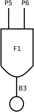
FIGURE 1. Simple oscillator instrument flowchart.
Unit generators do not have an action time and accept only symbolic data as parameters, which may be of three types.
• Note variables/parameters (Pn): these refer to instance-specific (scalar) data, with n as the index of their location in memory. These are shared between the instrument and the NOT statements that instantiate them. For example, P5 and P6 are the fifth and sixth parameter in a NOT statement (with NOT itself as P1, action time as P2, instrument as P3, and duration as P4).
• Audio buffers (Bn): these refer to global memory locations containing an audio buffer. By default these are 512-sample vectors. B1 and B2 are reserved for output use.
• Function tables (Fn): these refer to function tables defined by GEN statements.
In the particular case of the OSC unit generator, its first parameter is the signal amplitude (P or B); the second, its sampling increment (P or B); the third is the output buffer; the fourth is a function table; and the last is a scalar to hold the oscillator phase (its state). The OUT unit generator takes a buffer and adds it to the output bus (B1). The GEN statement defining function table 1 to hold a sine wave is.
GEN 0 2 1 1 1;
which creates F1 using the GEN subroutine 2 (designed to create one period of a waveform based on its Fourier series). Function tables are stored in 512-sample vectors by default.
Finally, a NOT statement to run instrument 1 for 5 s starting at time 0 is given as.
NOT 0 1 5 500 5.098;
This will play a sine wave at 440 Hz (if the sampling rate is set to 44,100) and peak amplitude set to 500. Since the signal was encoded using 12-bit signed integers, the maximum absolute amplitude is given as 2048. To compute a sampling increment from a given frequency in Hz, it is important to note that although function tables are 512 samples long, waveforms computed by GEN 2 complete a single cycle over 511 samples, one sample short of the total storage. Therefore the sampling increment Si for a given frequency f and sampling frequency fs is
despite the fact that the actual oscillator code wraps around over 512 samples. The reasons for this behaviour are not directly discussed by Mathews et al. (1969), although they observe that “[a]ctually only 511 numbers are independent since F(0) = F(511)” (Mathews et al., 1969, 50). In modern systems this is almost never the case. Waveforms are normally defined over the full length of the table, sometimes with an extra guard point added, as for instance in Csound (Lazzarini et al., 2016), for interpolation purposes. We expect that the mechanism of a shorter function length in MUSIC V may have been used for the same purpose. When restoring source code, it is important to check such details before any assumptions are made.
Since defining oscillator frequencies using sampling increments is not very convenient, conversions are often handled by user-supplied CONVT routines. MUSIC V facilitates the addition of Fortran code so that users can design these system components themselves. They can take, for instance, values supplied in the NOT statements and apply specific formulas such as the one in Eq. 1. Supplying the correct code for these subroutines is therefore essential for the correct interpretation of score parameters. For example, in many synthesis examples discussed in this paper, a CONVT routine applies conversion formulae to various Pn prior to these being supplied to the OSC unit generators. Therefore, when studying a MUSIC V score, to analyse the results correctly we need to take these formulae into account.
The MUSIC V operation is divided into three stages, or passes, which correspond to three Fortran source files in our codebase:
1. Pass 1 (pass1.f): the first stage parses the score file, checks for errors, and translates the input to a numeric form. Mnemonics are translated to integers and all the symbolic data is encoded as floating-point numbers with various offsets. The output is a text file containing newline-terminated lists of numbers.
2. Pass 2 (pass2.f): in this step, data is sorted in ascending execution time order, tempo processing and CONVT subroutines are applied to the inputs. Output is in a similar numeric format as the input.
3. Pass 3 (pass3.f): this is the acoustic compiler proper, which takes the instrument, function table, and note statements and executes them producing a digital audio waveform as output. Code for unit generators and GEN routines resides in this source file.
The development of our MUSIC V replica was based on a number of scattered source materials (Lazzarini et al., 2022b).
1. SAIL 1975 sources: in 2008, Bill Schottstaedt made available a machine-readable version of MUSIC V listings from the Stanford Artificial Intelligence Lab dating from 19/06/1975. This version included code for most parts of the software, with a number of modifications for the modern versions of the Fortran language. These included the replacement of most of the arithmetic IF statements in the code (these are deprecated but are still accepted by compilers such as gfortran), and a major reorganisation of pass 1 to deal with various memory models. It also included the change in the OSC code to allow for negative frequencies, as introduced by John Chowning (1973).
2. Risset’s Catalogue (Risset, 1969) contained the code for a number of subroutines that were missing in the SAIL 1975 sources.
3. The MUSIC V Manual (Mathews et al., 1969) provided a detailed description of the program as well as some code fragments that were used to complete and debug the code.
4. Complete listings of a 1968 version were found at the Fonds Jean-Claude Risset, which were important for situating the software as it existed at the time of the composition of Little Boy.
5. Scores of Little Boy provided some missing subroutines and additionally enabled the debugging of the complete system.
Through the methods of software archaeology (Hunt and Thomas, 2002) and supported by modern versioning tools, we were able to replicate the functionalities of the environment used by Risset in his composition and research. Also, based on this project’s findings, we could identify at least four distinct versions used at Bell Labs between 1968 and 1969 and a later one used at Stanford University:
1. Fonds Risset 1968 version, represented by the earliest extant source code. Parts of what we expected to be the released MUSIC V code are missing, and according to source code comments, some components are not functional or incorrect.
2. MUSIC V Manual version. This is based on the code and descriptions found in the Manual, the 1968 version, and the 1975 SAIL version, with modifications. It corresponds to what we can describe as the first released version of the system.
3. Little Boy version, for which no source code is available. This a hypothetical version constructed from the working components of the 1968 version, the edited Manual version, code fragments found in the Little Boy scores and the debugging procedures applied on these scores.
4. Catalogue version. This is based mostly on the Manual version with additions published as part of (Risset, 1969), and some modifications.
5. SAIL version: this is the source code from the SAIL listings. For this version, we only had access to the machine-readable version with modifications for modern fortran.
The initial work in reconstructing the software involved an assessment of the status of the SAIL 1975 sources and their modifications. This revealed that while the code could run simple scores and produce a predictable output, it could not handle a wider variety of material without extensive changes. This is a summary of the bug fixes and modifications that were applied to the sources to support the reconstruction work.
• In pass1.f, modifications made by Schottstaedt prevented the running of certain user-supplied PLF subroutines. The code was changed to enable this and to include the PLF3 subroutine provided by Risset (1969). A number of typos were corrected.
• In pass2.f, a major bug preventing the call of user-defined CONVT subroutines was fixed. The CON subroutine, which applied score-defined tempo changes, was broken and was restored by us. This work was essential to enable Little Boy scores to run correctly.
• In pass3.f, output was fixed to one channel (the STR stereo output unit generator was not functional), the sampling rate was hardcoded to 44,100 Hz. To allow to set the number of channels and sampling from the score, modifications to pass 3 and pass 1 code were required. Various bugs in unit generators were fixed and the interpolating oscillator code was restored based on the 1968 sources.
In addition to these changes, the compiler has been adapted to run within a modern operating system. The original workflow involved the score being prepared as a deck of punched cards, which together with the Fortran sources, were supplied to the computer as a batch job. The computation yielded a set of printouts (containing information about the pass, etc.) and the data output from each pass. This was fed to the subsequent pass, resulting in a digital audio file rendition. Within this workflow, it was possible to make additions to the Fortran source code in the form of user-supplied routines (e.g., PLF, CONVT, GEN). On a modern system, we work from pre-compiled binaries to avoid having to use the Fortran compiler for every score run. Also, it is more convenient to have a single driving command that can execute the three passes in sequence and produce a soundfile in a standard format.
To allow for these changes, the current project features the three passes to be invoked as routines from a single program. The code was written using the C language and included a component to translate the raw digital audio data into a RIFF-Wave soundfile format as a final step. In this form, a user only needs to supply the score file name and an output file name, and the three passes are run in sequence from a single command. Intermediary data is still preserved as separate files for inspection, and the main results can be opened with any current sound editing applications. Furthermore, as detailed later, a mechanism to select specific CONVT routines was introduced to facilitate the swapping of these without necessitating the recompilation of Fortran sources.
The practice of computer music is akin to running a simulation, in which users design computer algorithms and execute them with control data from computational scores (Keller et al., 2022). The result is a digital audio waveform. This set of procedures has two primary implications: from the point of view of musical design, computer-generated sound is the materialisation of an imagined music-world which does not need to abide by the rules of acoustic-instrumental thinking; from a software-design point of view musically oriented forms of computational thinking (Otero et al., 2020) may also foster the adoption of object-oriented programming paradigms (OOP).
MUSIC IV embodies OOP features that later became common in systems such as SIMULA (Lazzarini, 2013). OOP supports abstractions (instrument-classes and unit generators) which are instantiated to simulate sonic processes. These processes are key features of musical ecosystems. Two foundational texts of computer music (Tenney, 1963; 1969) document examples of the design of computational instruments through a musical approach to sound-synthesis techniques; pieces such as Little Boy provide another instance of the application of this knowledge. This conceptual and methodological perspective has triggered a body of qualitative changes in the practices of music creation and sharing with profound implications for technological design. In this section, we review a few notable examples that exemplify these developments.
An important design case within the 1961–1969 period is the use of modulation as a means to synthesise various time-varying spectra. The acoustic compiler provided an ideal environment for this, supporting multiple unit generators connected in various ways that could also handle control signals. With this software, Tenney was able to determine experimentally many important attributes of both amplitude and frequency modulation techniques (AM, FM), noting that they added “that element of richness” (Tenney, 1969, p.36) he required in his work. In this regard, he also noted that the use of bandlimited noise as a modulation source was more important than periodic signals, particularly in AM.
Amongst his experimental findings, the ones involving audio-range modulation seem to be particularly original. Tenney employed a random number generator to produce outputs at various frequencies, feeding this signal into the amplitude input of a sinusoidal oscillator to synthesise dynamically evolving noise bands. In this process, he was able to determine that the bandwidth of the noise region was defined by the rate of the random number generation, and that its centre frequency was defined by the oscillator frequency. While this is a heterodyning effect that was already known from radio-frequency theory, its application in digital audio was new and highly influential for future developments in sound synthesis.
Tenney’s pioneering work with audio-rate linear FM is also noteworthy. Although his experiments favoured the use of noise modulation, he was able to derive experimentally some important ideas that a decade later became part of FM synthesis theory (Chowning, 1973). Tenney notes that the bandwidth of FM is dependent both on the modulation range (or amplitude) and the noise-generation rate, whereas in the case of AM, the modulation range only affects the amplitude of the output sound (Tenney, 1963, 46). His conclusions agree with the fact that the modulation amplitude determines the maximum instantaneous frequency of the carrier signal and thus have such an effect. Tenney’s experimentally-derived formula for noise modulation indicates that the bandwidth is approximately determined by the sum of the range and rate of noise generation. As noted later by Chowning, the bandwidth of sinusoidal FM synthesis is dependent on the ratio of the frequency deviation to the frequency modulation called the index of modulation.
The experiments discussed by James Tenney (Tenney, 1963; 1969) are fully replicable. By following the explanations and flowcharts, it is possible to reconstruct the proposed designs on a modern system such as Csound. In his lab report (Tenney, 1969), Tenney provides a complete AM/FM testbed instrument. The following Csound code is a reconstruction of the AM/FM instrument as designed by Tenney (Tenney, 1969, 37). This instrument allows us to study the various forms of modulation explored in his experiments. In particular, it is possible to vary the noise rate (which is the frequency at which new random variables are produced) for both AM/FM modulators, the amount of noise AM as a fraction of total amplitude, and the amount of FM as fraction of the mean frequency. The instrument also includes a (sinusoidal) periodic FM source. In his description, there is no mention of any experiments using audio-range periodic FM, since he fixes the frequency of this sinusoid to 7.5 Hz (Figure 2).
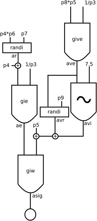
FIGURE 2. Tenney’s testbed instrument flowchart.
In the reconstruction of the original experiments (based on MUSIC III and MUSIC IV), the oscillators were not capable of negative sampling increments. Therefore the maximum FM width (the sum of periodic and random modulation amounts) cannot exceed 100% of the mean frequency, otherwise the reconstruction will not reproduce the original outputs. This is because the oscillators in Csound are capable of handling negative frequencies. The handling of negative frequencies was only introduced later in MUSIC V, following the development of the FM synthesis theory (Chowning, 1973).
0dbfs = 1
/*function tables, 512 samples long as in the original
gie - exponential decay to -60dB (amplitude)
give - trapezoid (frequency modulation)
giw - sawtooth waveform with 10 harmonics
*/
ilen = 512
gie ftgen 0,0,ilen+1,5,1,ilen,0.001
give ftgen 0,0,ilen+1,7,0,ilen*0.3,1,ilen*0.4,1,ilen*0.3,0
giw ftgen 0,0,ilen,10,1,1/2,1/3,1/4,1/5,1/6,1/7,1/8,1/9,1/10
/ * instrument parameters
p4 - amplitude (mean)
p5 - frequency (mean)
p6 - AM amount (percent/100)
p7 - AM noise rate (Hz)
p8 - max FM amount (percent/100)
p9 - FM noise rate (Hz)
*/
instr 1
ar randi p4*p6,p7
ae oscil ar+p4,1/p3,gie
ave oscil p8*p5,1/p3,give
avi oscil ave,7.5
avr randi ave,p9
asig oscil ae,avr+avi+p5,giw
out asig
endin
As part of our study of Risset’s Little Boy scores, we have also discovered a MUSIC V score fragment that features linear audio-rate periodic FM, as later employed by Chowning in works such as Stria (Zattra, 2007). To our knowledge, this is the earliest extant synthesis source-code demonstrating this technique. The same fragment also combines FM and feedback amplitude modulation (FBAM, which is discussed in the next section) to produce a complex time-varying spectrum. This design is not only quite unique, to the best of our knowledge it was neither discussed by Risset nor was it further explored in the literature. While, as we noted earlier, FM synthesis had already been introduced by Tenney, this example employs the kind of sinusoidal modulation which formed the core of John Chowning’s FM theory. The approach here is that of a sped-up vibrato, and while the modulation amounts are small (the index of modulation never exceeds 1.6), we have a clear example of the emergence of a characteristic FM synthesis spectrum.
The following MUSIC V score containing code extracted from one of Risset’s original scores (w20_003_2, p.42, dated 7 August 68, file name 1968_08_07_42debug.txt), shows the FM/FBAM code (for which a flowchart is shown in Figure 3). A single instrument is used, which includes a switch enabling FBAM in the second note of the score. The instrument contains four oscillators: the first two produce the amplitude and frequency envelopes for the modulation; the third is the modulator; and the fourth is the carrier. The FM amount (maximum instantaneous frequency deviation) and frequency increase over time and the audio-rate FM spectrum emerge towards the end of each note as the modulation rate rises to the audio range (reaching nearly 70 Hz). As indicated by the comments, the second note has the P10 parameter set to one, enabling feedback (this is used as a multiplier to the feedback signal). An analysis of the code and its output reveals a certain amount of aliasing (at 10 KHz sampling rate), which may be reduced with the use of higher sampling rates.
COMMENT: RISSET FM EXAMPLE EXTRACTED FROM LB MATERIALS;
SIA 0 4 10000;
COMMENT:VIBRATO VARIABLE POUR SONS DE CAMERA;
INS 0 2;
OSC P8 P7 B3 F3 P30;
OSC P9 P7 B4 F4 P29;
OSC B3 B4 B3 F2 P28;
AD2 P6 B3 B3;
MLT P10 B10 B5;
AD2 P5 B5 B6;
OSC B6 B3 B10 F2 P27;
OUT B10 B1;
END;
GEN 0 2 2 1 1;
GEN 0 1 3 .05 1 .05 10 .999 256 .999 512;
GEN 0 1 4 .1 1 .1 280 .999 512;
COMMENT:SANS FEEDBACK;
NOT 0 2 6 1000 554 0 20 70 0;
COMMENT:FEEDBACK;
NOT 7 2 6 500 554 0 20 70 1;
TER 14;
COMMENT:CONVT3
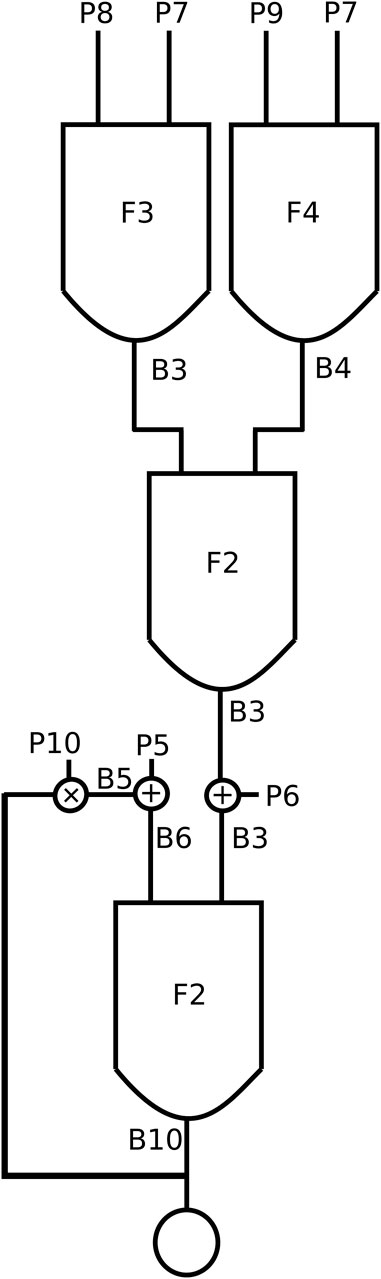
FIGURE 3. FM instrument flowchart.
Feedback amplitude modulation [as described in detail by Kleimola et al. (2011)] is another design case that emerged in early experiments with MUSIC V. In its simplest form, feeding back part of the signal from a sine wave oscillator to its amplitude input results in a significantly enriched spectrum with a brass-like quality (Layzer, 1973). These sounds could potentially be obtained through additive synthesis, however this demanded more computational resources. One of the reasons Risset extensively examined its sonic possibilities in his preparations for Little Boy was to achieve computationally efficient complex time-varying spectra. His use of FBAM hit a specific MUSIC V limitation: a fixed 512-sample feedback period was imposed by the design of the first version. Layzer (1973) notes that a later addition to the software was implemented by Richard Moore, making it possible for the period to be varied from 1 to 512 samples. However, no trace of this implementation was found in any of the sources we collected for our replica. To explore how this unit generator could have been used, we reconstructed this functionality in MUSIC V according to Layzer’s report.
Risset’s use of FBAM is characterised by the use of the instrument output buffer as the modulation input (i.e., replacing the noise source in Tenney’s example). This inserts a delay of 512 samples, the default size of audio buffers in MUSIC V, in the feedback path. Furthermore, since the software does not implement instance-unique memory for the signal buffers, instruments using feedback are not fully re-entrant, as instances do not have access to a fully separate dataspace. A side effect of this in Risset’s scores is that it is not possible to have simultaneously running instances of the same feedback AM instrument. The solution to this is to have several copies of the same instrument, one for each instance. Moreover, if instruments are to be executed serially, feedback buffer memory needs to be re-initialised through the use of dedicated memory-clearing instruments.
The example below is a fragment taken form one of the earliest FBAM examples by Risset (filename 1968_08_07_14debug.txt). The score has six instruments containing the same design, a single oscillator whose amplitude is modulated by its output, enabling up to six simultaneous sounds to be synthesised. Instruments 7 to 12 are used to clear the buffer memory for subsequent instances. These are run immediately before the end of the code section. Figure 4 shows the flowchart for instrument 1; instruments 2–6 are similar in design.
INS 0 1;
AD2 B7 P5 B3;
OSC B3 P6 B7 F1 P30;
STR B7 V1 B1;
END;
INS 0 2;
AD2 B8 P5 B3;
OSC B3 P6 B8 F1 P30;
STR B8 V1 B1;
END;
INS 0 3;
AD2 B9 P5 B3;
OSC B3 P6 B9 F1 P30;
STR B9 V1 B1;
END;
INS 0 4;
AD2 B10 P5 B3;
OSC B3 P6 B10 F1 P30;
STR V1 B10 B1;
END;
INS 0 5;
AD2 B11 P5 B3;
OSC B3 P6 B11 F1 P30;
STR V1 B11 B1;
END;
INS 0 6;
AD2 B12 P5 B3;
OSC B3 P6 B12 F1 P30;
STR V1 B12 B1;
END;
INS 0 7;
MLT B7 V1 B7;
END;
INS 0 8;
MLT B8 V1 B8;
END;
INS 0 9;
MLT B9 V1 B9;
END;
INS 0 10;
MLT B10 V1 B10;
END;
INS 0 11;
MLT B11 V1 B11;
END;
INS 0 12;
MLT B12 V1 B12;
END;
GEN 0 2 1 1 1;
STA 0 4 10000;
SV2 0 2 30;
SV2 0 30 0 120 12.5 120;
SV3 0 1 0;
NOT 1 1 6 200 103.8;
NOT 2 4 5 240 233;
NOT 2.75 2 4.25 350 174.6;
NOT 3 5 4 350 329.6;
NOT 3.5 3 3.5 300 440;
NOT 4.5 6 2.5 300 554.3;
NOT 8 12 .2;
NOT 8 11 .2;
NOT 8 10 .2;
NOT 8 9 .2;
NOT 8 8 .2;
NOT 8 7 .2;
SEC 9;
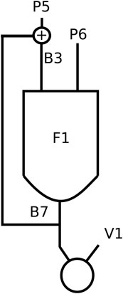
FIGURE 4. FBAM instrument flowchart.
According to Layzer’s description, Moore’s FBAM oscillator included an internal feedback path for amplitude modulation. Thus, the limitation of a fixed feedback interval is overcome. By accessing the output buffer, it is possible to work with delays of 1–512 samples. The following reconstruction is based on the existing code for OSC (including Chowning’s negative frequency modification), with the addition of two extra parameters: a feedback gain G and delay D (in samples). The Fortran code for this unit generator is shown below.
C FBAM OSCILLATOR
C FBM A,F,O,Fn,S,G,D
C G - feedback amount (0 - 1)
C D - delay in samples (P), 1 - 512
114 IDL = IFIX(FLOAT(I(L7))*SFI)
IF(IDL.gt.1) GOTO 1181
IDL = 1
GOTO 1182
1181 IF(IDL.lt.NSAM) GOTO 1182
IDL = NSAM
1182 SUM=FLOAT(I(L5))*SFI
IF(M1.gt.0) go to 1183
AMP=FLOAT(I(L1))*SFI
1183 IF(M2.gt.0) go to 1184
FREQ=FLOAT(I(L2))*SFI
1184 IF(M6.gt.0) go to 1185
G=FLOAT(I(L6))*SFI
1185 DO 1196 J3=1,NSAM
IPOS = MOD(J3 - 1 - IDL + NSAM, NSAM)
FDB = FLOAT(I(L3+IPOS))*SFI
J4=INT(SUM)+L4
F=FLOAT(I(J4))
IF(M2.gt.0) go to 1186
SUM=SUM+FREQ
GO TO 1190
1186 J4=L2+J3-1
SUM=SUM+FLOAT(I(J4))*SFI
1190 IF(SUM.GE.XNFUN)GO TO 1187
IF(SUM.LT.0.0)GO TO 1189
1188 J5=L3+J3-1
IF(M6.gt.0) go to 1192
GO TO 1193
1192 G=FLOAT(I(L6+J3-1))*SFI
1193 IF(M1.gt.0) go to 1194
GO TO 1195
1187 SUM=SUM-XNFUN
GOTO 1188
1189 SUM=SUM+XNFUN
GO TO 1188
1194 J6=L1+J3-1
AMP = FLOAT(I(J6))*SFI
c out = (a + g*out[n-d])*f[ndx]
1195 I(J5)=IFIX((AMP+FDB*G)*F*SFXX)
1196 CONTINUE
I(L5)=IFIX(SUM*SFID)
RETURN
This oscillator can be used as a replacement to Risset’s external buffer feedback, with D set to 512 samples. Note that since the re-entrancy issue noted before is a system-design condition, there is no means for a unit generator to have access to a separate per-instance dataspace. While this UG allows the feedback period to be adjusted, it still cannot be used in parallel runs of the same instrument.
An example of the use of this unit generator is featured in the following MUSIC V score, with two sounds produced with the same parameters and with different delays (512 and 1 samples). The use of a 1-sample delay produces the expected spectrum as given by Layzer. The 512-sample feedback approximates this outcome but it does not match it. The output is louder due to the summing effects (Kleimola et al., 2011).
COM: FBAM UG EXAMPLE;
INS 0 1 ;
OSC P7 P9 B4 F3 P31 ;
OSC P5 P9 B3 F2 P32 ;
FAM B3 P6 B2 F1 P30 B4 P8;
OUT B2 B1 ;
END ;
GEN 0 1 3 1 0 .9 100 .1 411 0 511 ;
GEN 0 1 2 .999 0 .999 50 .999 411 0 511 ;
GEN 0 2 1 512 1 1 ;
NOT 1 1 5 250 5.0984 0.9 512 0.0023;
NOT 6 1 5 250 5.0984 0.9 1 0.0023;
TER 12.00 ;
We conducted two case studies involving the reconstruction of software and the implementation of sonic examples. The first study applied our replica of the MUSIC V compiler to render the original Little Boy MUSIC V scores (Risset, 1968; Lazzarini et al., 2022a) as well as the FBAM examples discussed earlier. The second study features the use of a modern music-programming environment, Csound 6, to reconstruct a composition from scratch following the design instructions given by James Tenney. These two approaches exemplify a-ubimus techniques potentially applicable to both the creative processes and products of a large number of digital artworks produced during the 1960s and 1970s.
Our target is to reconstruct the sonic materials through the use of original software. In situations where developing a replica is not practical or methodologically appropriate, we resort to currently available software or hardware environments, for instance, Csound (Lazzarini et al., 2016), as we have done earlier in the study of modulation synthesis experiments. When reconstructing computer-music products of the 1961–1969 period, the choice of Csound is not arbitrary: this language sits at the end of a development line directly connected to the first acoustic compiler (MUSIC III). Additionally, its backward compatibility fosters the preservation of musical assets. This characteristic sets it apart from other computational tools and points to a close relationship between sustainability and community-based development.
The process of testing the sources of Little Boy was essential to fine-tune the functionality of MUSIC V. Thus, the a-ubimus reconstruction of the musical material was an integral component of the implementation of the replica. Resynthesizing the forty six preserved score printouts of Little Boy involved a process of debugging both MUSIC V and Risset’s code. These procedures included a detailed critical analysis of the musical data and syntax, encompassing parameters such as pitch, duration, dynamics, timbre, and also organising and annotating the extra-musical information featured in the commented code, while searching for original synthesis methods and relevant sonic examples.
Following the synthesis of each score, the following step was to compare the rendered audio with the expected aural results, taking into consideration Risset’s annotations scattered in several Fonds documents as well as checking the autograph recording of the piece (Risset, 1988). Despite all these precautions, in many cases the original scores did not produce satisfactory results. Two typical situations arose stemming from (a) execution errors or (b) design errors. In the first case, no audio output was obtained and an error message was reported. This type of failure may be due to a missing parameter or command in the score, the existence of mismatched parameters, or bugs in the Fortran source code. Conversely, when a design error arises, MUSIC V may produce audio that does not match the composer’s planned results. In this case, it may be that: (a) the values in the score were incorrect or (b) the instrument construction was flawed.
While the above two categories are likely Risset’s errors, another group of issues is related to problems in the MUSIC V source code. These may arise from simple transcription mistakes, missing subroutines, or may be due to mismatches between code versions. Some of these problems become evident when the audio output is faulty despite the accuracy of Risset’s code. We observed this issue during the analysis of the function table generators (GENs), an essential part of the synthesis architecture.
As noted earlier, the process of debugging the original Little Boy material revealed the existence of various versions of MUSIC V. The fact that the system was developed at the same time as the piece was being composed meant that some software components were adopted on a score-to-score basis. We had to develop means to track these changes so that the scores were aligned with their corresponding compiler versions. After the public release of the first official version of the system in 1969, MUSIC V became available to other computer-music facilities beyond Bell Labs, and further modifications were made to the software (such as the support of negative sampling increments).
We started by assuming the preserved Little Boy scores were running correctly at Bell Labs, meaning they were free of execution errors. From this standpoint, the objective became making them compatible with our replica without involving major modifications. The guideline principle is to intervene as little as possible, while modifying the source code to match the score. However there are cases where it is not possible to make this assumption because it is necessary to have a broad understanding of the composer’s intentions, the software, and the results expected. As an example, we outline the handling of an original score including the execution, design and source-code errors. In this discussion, we use the score dated 5 August 68, p.36, as the source. The first run of the code yields an error.
Where is Harvey, pass1 failed. Instrument definition incomplete.
Debugging identified this as a missing oscillator (OSC) in the instrument. We added an OSC statement as used in a similar score (dated from 7 August 1968, p.14). While this allowed the code to run correctly in pass 1, it resulted in a segmentation fault.
end of pass2. segmentation fault: 11.
The analysis of the score pointed to a function 1 (F1) used by that OSC that was missing. Adding GEN 0 2 1 1 1 allowed a successful run and an audio file was created. However, the resulting sound did not correspond to what was expected. Further inspection showed that the Fortran code for the CONVT routine was incorrect: two lines of the code were missing. Once a fix was applied, a waveform with the expected characteristics was produced, but with an inverted stereo image. This result pointed to a bug in the Fortran code for pass 3, where the output buffer had an extra offset of one sample. This issue was solved yielding the expected spatial placement.
C 99 J=IDSK+1
C VL: this was IDSK+1 it was offsetting the stream
C by 1
C and inverting the stereo image
99 J=IDSK
M1=IP(10)
M2=0
ISC=IP(12)
The next intervention in the score was due to a missing SIA statement. In Risset’s scores, this resource is used to set the sampling rate. If it is missing, the default value of 44.1 KHz is employed, as defined in the source code for pass 3. We realised that such a sampling rate was never used at Bell Labs (as their digital-to-audio converter could not handle it). Analysis of the 1968 sources indicated that the default value was originally 10 KHz, and we suspect the modification to 44.1 KHz was done later in the SAIL sources (or by Schottstaedt in his transcription of them). We fixed this first by adding a SIA statement, setting the correct sampling rate, and added a comment to the score noting this. Later in the process, we restored the default sampling rate to 10 KHz and thus, the score is rendered as originally designed regardless of the presence of a SIA line in the score.
Finally, an outstanding error which had been already identified by the composer was found in one of the NOT statements. Risset’s handwritten annotation indicates that a value needs to be modified. The following is the fully debugged score file, which resulted from these corrections (RVN marks our added comments),
COMMENT: header pencil JCR 08/05/68 ;
COMMENT: header pencil JCR T1678 M2994 ;
COMMENT:FANFARE POUR LE TRIOMPHE;
COMMENT:100 PER CENT FEEDBACK;
COMMENT: RVN OSC is missing in all INS ;
COMMENT: RVN added this to each
instrument OSC B3 P6 B7 F1 P29 STR B7 V1 B1 END;
INS 0 1;
SET P10;
ENV P5 F2 B3 P7 P8 P9 P30;
AD2 B3 B7 B3;
COMMENT: RVN in each INS definition the 3 lowest lines are added - OSC STR and END;
OSC B3 P6 B7 F1 P29;
STR B7 V1 B1;
END;
INS 0 2;
SET P10;
ENV P5 F2 B3 P7 P8 P9 P30;
AD2 B3 B8 B3;
OSC B3 P6 B8 F1 P29;
STR B8 V1 B1;
END;
INS 0 3;
SET P10;
ENV P5 F2 B3 P7 P8 P9 P30;
AD2 B3 B9 B3;
OSC B3 P6 B9 F1 P29;
STR B9 V1 B1;
END;
INS 0 4;
SET P10;
ENV P5 F2 B3 P7 P8 P9 P30;
AD2 B3 B10 B3;
OSC B3 P6 B10 F1 P29;
STR V1 B10 B1;
END;
INS 0 5;
SET P10;
ENV P5 F2 B3 P7 P8 P9 P30;
AD2 B3 B11 B3;
OSC B3 P6 B11 F1 P29;
STR V1 B11 B1;
END;
INS 0 6;
SET P10;
ENV P5 F2 B3 P7 P8 P9 P30;
AD2 B3 B12 B3;
OSC B3 P6 B12 F1 P29;
STR V1 B12 B1;
END;
SIA 0 4 10000;
COMMENT: RVN added SIA above otherwise it would use 44100Hz ;
SV3 0 1 0;
COMMENT: RVN added GEN 2 for function F1 in the line below;
GEN 0 2 1 1 1 ;
GEN 0 1 2 0 1 .8 85 .8 105 .999 128 .8 256 .33 285 .12 333 0 384 0 512;
GEN 0 1 3 0 1 .75 128 .6 140 .999 256 .3 280 .13 325 0 384 0 512;
COMMENT: RVN two line above are too long causing an error if not split into two lines (probably due to 72-char limit);
NOT 1.0 1 .9 300 329.6 .06 1 .15 0;
NOT 1.5 4 .9 250 523.2 .06 1 .15 0;
NOT 2.0 1 .9 300 440.0 .06 1 .15 0;
NOT 2.5 4 .9 250 622.2 .06 1 .15 0;
NOT 3.0 1 .9 300 329.6 .06 1 .15 0;
NOT 3.5 4 .4 250 554.3 .04 1 .1 0;
NOT 4.0 4 .9 250 523.2 .06 1 .15 0;
NOT 4.5 1 .9 300 440.2 .06 1 .15 0;
NOT 5.0 4 .9 250 622.2 .06 1 .15 0;
NOT 5.51 1 .9 300 349.2 .06 1 .15 0;
NOT 6.0 4 .9 240 830.0 .06 1 .15 0;
NOT 6.5 1 .9 280 523.2 .06 1 .15 0;
NOT 7.0 4 .5 230 740 .04 1 .1 0;
NOT 7.5 4 .99 215 923.3 .05 1 .1 0;
COMMENT: l.a. pencil JCR 923.3 corrected to 932.3;
COMMENT: RVN we left it as in the printout;
NOT 8 1 .49 200 440 .03 1 .1 0;
NOT 8.5 1 4.25 400 103.8 .06 3 .18 3;
NOT 9.25 4 3.50 400 146.8 .04 2 .17 3;
NOT 9.5 2 3.25 400 164.8 .05 2 .16 3;
NOT 10.0 5 2.75 400 196.0 .04 2 .15 3;
NOT 10.5 3 2.25 400 233.1 .04 1 .14 3;
NOT 11.0 6 .75 400 277.2 .04 1 .13 3;
TER 14;
COMMENT: CONVT 4;
COMMENT: margin pencil JCR .0086 399 samples out of range ;
COMMON IP(10),P(100),G(1000)
IF(P(1).NE.1.)GOTO100
COMMENT: RVN CONVT is missing the beginning I added two lines above;
F=511./G(4)
FE=F/4.
P(6)=F*P(6)
P(8)=P(4)-P(7)-P(9)
IF(P(8))2,3,4
2 P(7)=(P(7)*P(4))/(P(7)+P(9))
P(9)=(P(9)*P(4))/(P(9)+P(7))
3 P(8)=128.
GOTO5
4 P(8)=FE/P(8)
5 P(7)=FE/P(7)
P(9)=FE/P(9)
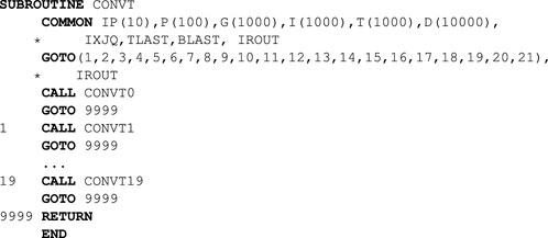
100 RETURN
END
AT flowchart for instrument 1 is given in Figure 5. This is an FBAM instrument, similar to the one discussed earlier (see Figure 4), but with the addition of a trapezoidal amplitude envelope. The parameters P7, P8, and P9 determine, attack, steady state, and decay times, respectively. The shape of each of these segments is given by the first, second, and third quarters of F1, and the maximum amplitude is given by P5. Instruments 1-6 are similarly designed.
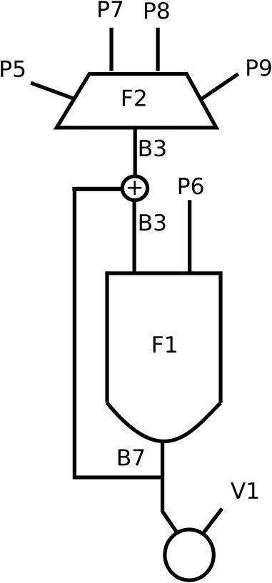
FIGURE 5. Fanfare instrument flowchart.
The CONVT routines presented an important challenge during the reconstruction process. As noted earlier, the MUSIC V architecture allows the users to include their own CONVT code in Fortran. Typically these are used to set the sampling increment for a given frequency, or to set the envelope duration which is dependent on the length of the function table and the sampling rate. While the function table length is hard-coded in MUSIC V to 512 samples, the sampling rate may be defined by the user in each individual score (as discussed in the previous section). Score-specific sampling rate conversions can be applied individually and present a powerful tool for a composer. They allow for the control of tempo, AM/FM depth and modulation ratio, among other parameters.
For example, in Risset’s FANFARE POUR LE TRIOMPHE score, a specific CONVT routine is given, in which the P array holds the NOT parameters, the IP array contains system constants, and the G array takes any user-defined configurations, such as the sampling rate [G(4)]. This CONVT takes P(6) (oscillator frequency, given originally in Hz in the score), translates it into a sampling increment value, and replacing P(6) in the converted score. It also takes the values of P(7)–P(9) and converts them into segment durations for the envelope generator, using P(4) (total duration) and the sampling rate. Since the envelope generator uses quarter-table lengths for each segment, the CONVT routine scales their durations accordingly.
In the case of the Little Boy sources, many different CONVT functions were given together with the MUSIC V score, which are essential for the correct interpretation of the code. Faced with the task of swapping CONVT routines for every score, for practical reasons, we opted to add a means of choosing pre-compiled CONVT functions directly from the score. With this approach, any new CONVT that we encountered could be added and kept in the Fortran sources, provided that we associated these with a unique number. Once a CONVT is added to pass2 it can be called by placing a command inside a comment after the last line of the code:
COMMENT: CONVT < convt number>;}
This enables the running of scores with different CONVTs without having to modify pass 2 at each run. If no CONVT is specified at the end of the score, CONVT 0, a general subroutine from the Catalogue, is called. This mechanism is implemented thus.
1. Since a COMMENT is ignored in pass 1, there is no need to modify the score parser.
2. Fortran code for each pass is called as functions from a C-language frontend. This code takes care of parsing the comment statement identifying the CONVT routine number.
3. When the pass 2 function is called, this is passed as an argument, and stored in a global (COMMON) variable, IROUT.
4. The CONVT routine in pass 2 is supplied as an entry point to the various subroutines,
The pass 2 code for the Little Boy-version replica contains twenty different CONVT subroutines, which Risset used for his forty-six Little Boy scores.
The GEN routines generate the 512-sample tables used by the unit generators. Since their usage is inconsistent in the observed code, GEN issues were one of the most common sources of errors. In SAIL and Manual versions, GEN 1 indexes the stored samples from 0 to 511. GEN 1 from the Catalogue, Fonds Risset 1968, and Little Boy code expect indices to be defined in the [1,512] range. When used to define the amplitude envelope, these differences may result in incorrect outputs. Restoring the GEN 1 code to match the 1968 sources was therefore essential to render the source audio waveforms from Little Boy.
Further issues with GEN routines are due to changes in different versions of the source code. SAIL (as well as the MUSIC V Manual) code contained only GEN 1 and GEN 2. To run the Little Boy scores, we added GEN 3 to GEN 8. Their source code is published in Catalogue (GEN5 excluded) (25). At Bell Labs, GEN 5 was used only to invoke a system-dependent routine to skip files on the magnetic tape, so no code for this was included in the Catalogue. However, we discovered that Little Boy scores use GEN 5 to compute function tables (as usual), which corresponded to the GEN 7 code given in Risset 1969. Depending on the role of GEN 5 in the instrument definition, running these scores would cause either a segmentation fault or result in no audio or an audio file with faulty sound. Here is the code for GEN 7, renamed to GEN 5 as it is used in Little Boy scores.
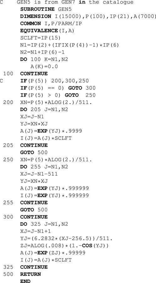
Since GEN 5 is used as an exponential function generator, file-skipping in Little Boy is done using GEN 3 or GEN 4. However, both are also used to design tables, so they cannot be applied to skip files. This limitation probably led to designing a dedicated GEN for skipping files in later versions. Since we could not solve these ambiguities by changing the Fortran source code, our approach was to modify the score and comment out the lines in question. Here is an example from 1968_11_01_160debug.txt:
COMMENT:TO SKIP FILES 1 AND 2;
COMMENT:GEN 0 4 2;
COMMENT: RVN l.a. commented out - no need for skipping files ;
For Ann (Rising) is a Tenney composition from 1969. Its first complete version employed a computer-synthesised sine wave glissando edited and mixed using analogue tape-based studio methods (Tenney, 1984). This was superseded by a software reconstruction created by Tom Erbe (Erbe, 2018) using Csound. An analysis of the source code of this reconstruction identified a fencepost bug, which results in an extra set of glissandi that produce an unintended doubling of some of the sine waves. We developed a new replica using the latest version of Csound, which corrects this issue and also provides the means to obtain new versions derived from the original concept. Both of these goals are achieved by a terse representation of Tenney’s design.
This piece consists of 240 sine wave glissandos over several octaves, each starting at the subsonic frequency threshold and rising towards the human-hearing limit. The amplitude of each glissando is shaped by a trapezoidal envelope. While this pattern resembles the tones synthesised by Tenney and Risset to support Shepard’s research on the circularity of pitch perception (Shepard, 1964), the motivation and approach here follow distinct lines. The compositional intention is not to explore the fusion of the sine tones into a continuous glissando with no discernible start or end. On the contrary, Tenney creates a perceptual space where the listener’s focus can alternate between the individual trajectories of each glissando and the fused spectrum (Wannamaker, 2022).
This experiential ambiguity is achieved because the glissandi are not spaced by octaves. The original tape version and the original reconstruction adopted a minor-sixth interval
The following code was used by Tom Erbe in his reconstruction of the piece, which appeared in the CD release James Tenney: Selected Works 1961–1969 (New World Records 805,702, 1993). According to Polansky (1983), the code was written from a description given by the composer, who also suggested the slight modification of extending the glissandos for one extra octave (to 14,080 Hz). This version was prepared by Matt Ingalls, who transferred Erbe’s code to a CSD file format (as used in later versions of Csound), as a first step to prepare a 15-channel performance of the piece (premiered at the San Francisco Tape Festival, 26 January 2007). The code listing below removes the middle section of the score for brevity, but we retain Ingall’s comment at the end. This indicates the fencepost error and duly comments out the offending lines.
<CsoundSynthesizer>
<CsInstruments>
sr=44100
kr=441
ksmps=100
instr 1
kf expon 40,33.6,10240
ka linseg 0,8.4,2000,16.8,2000,8.4,0
a1 oscil ka,kf,1
out a1
endin
</CsInstruments>
<CsScore>
f1 0 16384 10 1
i1 0 42
i1 +
i1
i1
i1
i1
i1
i1
i1
i1 2.8 42
i1 +
i1
i1
i1
i1
i1
i1
i1
i1
(...)
i1 39.2 42
i1 +
i1
i1
i1
i1
i1
i1
i1
i1
e -- matt: i stopped it here as the next notes will
overlap the 1st ones.
i’m not sure if this is Tenney’s or Erbe’s doing,
but i assume this is not the intent.
i wonder if it can be heard on the Artifact CD or not?
i1 42.0 42
i1 +
i1
i1
i1
i1
i1
i1
i1
i1
</CsScore>
</CsoundSynthesizer>
Our new reconstruction uses the latest version of Csound. This code distils Tenney’s design to a minimum set of code statements, as permitted by the language. By means of a recursive approach, it is possible to arrive at three distinct statements.
1. The synthesis of the sine wave glissando, using an oscillator controlled by amplitude and frequency time functions.
2. The scheduling of the successive glissando instances.
3. A single statement to prime the recursive mechanism.
In addition to these statements, the Csound syntax requires that we wrap each instance of the glissando in an instrument block. The complete code can therefore be given as five lines. In order to facilitate the adjustment of the spacing between glissandos, macro replacement is employed (using Csound’s language preprocessor). The example below sets this frequency interval to the golden ratio, which is, amongst other things, the limit of the sequence of ratios of consecutive terms in the Fibonacci series (1:1, 2:1, 3:2, 5:3, 8:5, …). According to Tenney, this choice would make the difference tones among pairs of glissandi to be already contained in the lower tones, thus producing a smoother, or more perfect, version of the piece (Polansky, 1983). We should also note that this spacing avoids the appearance of octaves, which is not the case when using the 12TET sixth: this interval divides two octaves into three equal parts, thus every fourth glissando produces an octave doubling (this in fact could help the perception of the pitch circularity).
A flowchart for the Csound instrument is given in Figure 6.
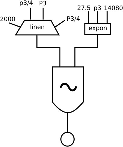
FIGURE 6. For Ann instrument flowchart.
#define INT #log2((1+sqrt(5))/2)#
instr 1
out(oscili( linen:a(2000,p3/4,p3,p3/4), expon:a (27.5,p3,14080)))
schedule(1,4.2*$INT, times:i() < 4.2*$INT*240 ? 37.8 : 0)
endin
schedule(1,0,37.8)
We should note that this code can be run via a frontend or an integrated development environment, wrapped in a CSD file, or sent as a string via a UDP/IP message to a Csound server. It will run the piece as designed by Tenney, with 240 glissandos. It is also possible to produce a realtime performance which, by removing the duration check, may be infinite.
times:i() < 4.2*$INT*240 ? 37.8 : 0
A feature of this reconstruction is the compactness of its computational design. While the original reconstruction used many lines of code to achieve a comparable sonic result, by adopting modern programming techniques, we arrived at a terse representation of the composition. Such an approach is less prone to errors, since these become more readily identifiable. While in this case a terse representation is preferable as it encapsulates the underlying compositional thinking precisely, this is not guaranteed to be universally true. In some situations, it may have the opposite effect: how expansive or how economical the computational resources should be to support legibility, consistency, and sharing is still an open research question.
The archaeological ubimus procedures and the results outlined in this paper point to a set of issues that were not addressed by the early computer-music practitioners. As highlighted by the drastic changes in the technological landscape of the last three decades, these issues have remained dormant despite their relevance [see (Keller et al., 2014; Lazzarini et al., 2020b) for a detailed discussion of emerging challenges]. Having discussed several caveats in the previous sections, we should stress the novelty and specificity of the knowledge yielded by Tenney and Risset’s musical experiments carried out between 1961 and 1969. The explorations prompted by For Ann (Rising) hint at music creation as a driver for what is nowadays known as practice-based or practice-led research (Candy, 2019). As suggested by Gaver and other referents of interaction design (Gaver et al., 2003), although not fitting comfortably within the context of utilitarian-design goals, ambiguity is an increasingly important aspect of human-computer interaction. This quality was consciously pursued by Tenney, pioneering complementary aesthetic and empirical insights on the subtle relationships between time and timbre within artistic practice (Wannamaker, 2021), cognitive science and interaction design (Löwgren, 2009).
Risset’s Little Boy project encompasses the development of new digital synthesis techniques, the various attempts to emulate acoustic-instrumental sources and a careful dialogue with extra-musical artistic elements, including theatrical performances and contextual pointers. This places such early computational approaches to music-making at least on an equal footing with the analogue-studio electroacoustic work of the previous decade. However, neither Little Boy nor For Ann (Rising) could have been fully achieved within the standard analogue studio. On the same vein and through the archeological ubimus prism, a subtle and long lasting impact of both practitioners can be inferred. In particular, Tenney’s contributions have been overlooked by the mainstream computer-music discourse [cf Polansky (1983); Wannamaker (2021; 2022) for notable exceptions].
Defined as an ecology encompassing socio-technical stakeholders that form part of cognitively and socially situated niches (Keller et al., 2014), ubiquitous music has fostered investigations on the properties that emerge from interactions during musical activities. These properties are rarely available through the analysis of musical products. Consequently, ubimus methods tend to target the deployment of computational prototypes. This is also the strategy adopted in archaeological ubimus. By designing and deploying replicas of technological relics, we gain insights on the circulation of knowledge enabled by ly reconstructed ecosystems. The two cases presented are examples of its potential contributions and point to several new avenues for future research.
As highlights of this project, we have documented the following items: a working replica of one of the earliest music-programming languages, MUSIC V; the recovery, adaptation and deployment of the original MUSIC V scores of Little Boy, located in the Fonds Risset; the implementation of a refined version of FBAM synthesis in MUSIC V; a high-quality, error-free rendition of For Ann (Rising) by means of a distilled prototype of Tenney’s computational proposal; and the implementation and documentation of a new For Ann (Rising) version based on Tenney’s concept of golden-ratio spectral spacing.
The procedures adopted throughout this project indicate the need to recalibrate the roles of the stakeholders in the design of information technology. The evidence gathered points to an ongoing process of circulation of knowledge which materialises in creative procedures, musical products and code. The specifically musical demands that impact information-technology ecosystems become explicit in For Ann (Rising) and Little Boy. Tenney’s approach highlights the roles of ambiguity and terseness in the design of technological constructs. These relational properties have emerged as relevant aspects of recent endeavours in computational design for creative aims. The usage of simulations, as exemplified in Little Boy, is gaining momentum as a strategy to deal with highly complex cognitive demands.
In this article, we have applied the methods of a-ubimus to explore some key aspects of early computer music, 1961–69. In this period, we have observed some seminal developments, such as the first exploration of digital audio processing techniques like FM and FBAM. Our approach was twofold: where our investigations yielded recoverable original source code we attempted to realise these directly (via our MUSIC V replica); complementary, when this was not possible we relied on the recreations of original textual descriptions, annotations, and graphical illustrations coded using modern software. This process, as detailed in the paper, allowed us not only to evaluate the impact of these developments in music, but also to ask new questions about the relationship between the practitioners and the technologies they adopted and fostered.
Imagined sonic worlds that are actionable, shareable and meaningful for human interactions may potentially emerge from current ubimus investigations. Explorations of the affordances of these simulated environments complement the long-standing usage of music-making as a symbolic playground for social interactions. Whether this potential will be employed to advance an agenda of solidarity, respect for diversity and preservation of cultural and environmental assets depends on the ethical scaffold of the artistic approaches. Ubimus endeavours have actively pursued a socially responsible, planet-friendly and very cautious attitude toward the incorporation of information technology in everyday life. We hope that the ubimus-archaeological techniques and results presented in this report will help to advance these community-oriented perspectives.
The original contributions presented in the study are publicly available. This data can be found here: https://github.com/vlazzarini/musicv.
All authors contributed equally to conception and design of the studies presented in this paper. Archival research and reconstruction of Little Boy scores was carried out by NR and the FORTRAN/C coding for the reconstruction of MUSIC V by VL. The writing of the manuscript was shared equally by all the authors. All authors contributed to manuscript revision, read, and approved the submitted version.
DK acknowledges support from the Brazilian Research Council CNPq [202559/2020–3]. NR acknowledges support from the SNSF through the HKB BFH project “In Hommage from the Multitude,” grant number 178833.
We would like to thank Fonds Jean-Claude Risset (PRISM, CNRS Marseille) and Dr. Vincent Tiffon for their support; Bill Schottstaedt for the machine-readable version of the 1975 MUSIC V sources; and Matt Ingalls for the 1993 For Ann realization Csound sources.
The authors declare that the research was conducted in the absence of any commercial or financial relationships that could be construed as a potential conflict of interest.
All claims expressed in this article are solely those of the authors and do not necessarily represent those of their affiliated organizations, or those of the publisher, the editors and the reviewers. Any product that may be evaluated in this article, or claim that may be made by its manufacturer, is not guaranteed or endorsed by the publisher.
Candy, L. (2019). The creative reflective practitioner: Research through making and practice. London: Routledge. doi:10.4324/9781315208060
Chowning, J. (1973). The synthesis of complex audio spectra by means of frequency modulation. J. Audio Eng. Soc. 21, 527–534.
David, J., Mathews, M. V., and McDonald, H. S. (1959). “A high-speed data translator for computer simulation of speech and television devices,” in Proceedings of the Western Joint Computer Conference, San Francisco, California, 169–172.
Doornbusch, P. (2004). Computer sound synthesis in 1951: The music of CSIRAC. Comput. Music J. 28, 10–25. doi:10.1162/014892604322970616
Erbe, T. (2018). Some notes on for Ann (rising). Available at: http://musicweb.ucsd.edu/∼terbe/wordpress/ (Acessed on 10 15, 2022).
Gaver, W. W., Beaver, J., and Benford, S. (2003). Ambiguity as a resource for design. In Proceedings of the SIGCHI Conference on Human Factors in Computing Systems (CHI 2003), Ft. Lauderdale, Florida (Fort Lauderdale, FL: ACM)), 233–240. doi:10.1145/642611.642653
Hiller, L. A., and Isaacson, L. M. (1957). Illiac suite for string quartet [score] (Bryn Mawr, PA: Theodore Presser Company).
Hiller, L., and Isaacson, L. M. (1959). Experimental music: Composition with an electronic computer. New York, NY: McGraw-Hill.:
Keller, D., Lazzarini, V., and Pimenta, M. S. (2014). XXVIII of computation music series. Berlin and Heidelberg: Springer International Publishing. Ubiquitous Music, vol. doi:10.1007/978-3-319-11152-0:
Keller, D., Radivojević, N., and Lazzarini, V. (2022). “Issues of ubimus archaeology: Beyond pure computing and precision during the analogue-digital transition,” in Proceedings of the Ubiquitous Music Symposium (UbiMus 2022), Curitiba, PR (Curitiba, Brazil: Ubiquitous Music Group), 17–26.
Kelly, J., Lochbaum, C., and Vyssotsky, V. (1961). A block diagram compiler. Bell Syst. J. 40, 669–676. doi:10.1002/j.1538-7305.1961.tb03236.x
Kleimola, J., Lazzarini, V., Välimäki, V., and Timoney, J. (2011). Feedback amplitude modulation synthesis. EURASIP J. Adv. Signal Process. 2011, 434378. doi:10.1155/2011/434378
Layzer, A. (1973). Some idiosyncratic aspects of computer synthesized sound. In Proceedings of the American Society of University Composers. 27–39.
Lazzarini, V. (2013). The development of computer music programming systems. J. New Music Res. 42, 97–110. doi:10.1080/09298215.2013.778890
Lazzarini, V., and Keller, D. (2021). Towards a ubimus archaeology. In Proceedings of the Workshop on Ubiquitous Music (UbiMus 2021), Porto, Portugal (Porto, Portugal: Ubiquitous Music Group), 1–12. doi:10.5281/zenodo.5553390
Lazzarini, V., Keller, D., Otero, N., and Turchet, L. (2020a). Ubiquitous music ecologies. London: Taylor & Francis.
Lazzarini, V., Keller, D., and Radivojević, N. (2022c). “Issues of ubimus archaeology: Reconstructing Risset’s music,” in Proceedings of the Sound and Music Computing Conference, St.Etienne, France (St-Étienne, France: Université Jean Monnet), 107–114.
Lazzarini, V., Keller, D., and Radivojević, N. (2022b). Little Boy by jean-claude Risset – reconstructed.
Lazzarini, V., Yi, S., Ffitch, J., Heintz, J., Brandtsegg, O., and McCurdy, I. (2016). Csound: A sound and music computing system. 1st edn. Berlin: Springer.
Löwgren, J. (2009). Toward an articulation of interaction esthetics. New Rev. Hypermedia Multimedia 15, 129–146. doi:10.1080/13614560903117822
Mathews, M., and Guttman, N. (1959). “The generation of music by a digital computer,” in Proceedings of the 3rd International Congress on Acoustics, reprinted in The Historical CD of Digital Sound Synthesis, Stuttgart, Germany, 30–34.
Mathews, M. V. (1961). An acoustic compiler for music and psychological stimuli. Bell Syst. Tech. J. 40, 677–694. doi:10.1002/j.1538-7305.1961.tb03237.x
Mathews, M. V., Miller, J. E., Moore, F. R., Pierce, J. R., and Risset, J. C. (1969). The technology of computer music. Cambridge, MA: The MIT Press.
Otero, N., Jansen, M., Lazzarini, V., and Keller, D. (2020). “Computational thinking in ubiquitous music ecologies,” in Ubiquitous music ecologies. Editors V. Lazzarini, D. Keller, N. Otero, and L. Turchet (London: Routledge), 146–170. doi:10.4324/9780429281440
Pinkerton, R. C. (1956). Information theory and melody. Sci. Am. 194, 77–87. doi:10.1038/scientificamerican0256-77
Risset, J.-C. (1969). An introductory catalogue of computer-synthesized tones. Murray Hill, NJ: Bell Labs.
Risset, J.-C. (1968). Original MUSIC V code for little Boy (W20_003_2). Marseille, France. Fonds Jean-Claude Risset, Laboratoire PRISM (UMR7061)).
Shepard, R. (1964). Circularity in judgments of relative pitch. J. Acoust. Soc. Am. 36, 2346–2353. doi:10.1121/1.1919362
Tenney, J. (1963). Sound-generation by means of a digital computer. J. Music Theory 7, 24–70. doi:10.2307/843021
Tenney, J. (1984). The music of James Tenney: Selected works 1963-1984. Toronto, Canada: Musicworks.
Wannamaker, R. (2021). The music of James Tenney, volume 1: Contexts and paradigms. Champaign, IL: University of Illinois Press.
Wannamaker, R. (2022). The music of James Tenney, volume 2: A handbook to pieces. Champaign, IL: University of Illinois Press.
Keywords: computer music, reconstruction, sound synthesis, computer music languages, MUSIC V, ubiquitous music archaeology, a-ubimus
Citation: Lazzarini V, Keller D and Radivojević N (2023) Issues of ubiquitous music archaeology: Shared knowledge, simulation, terseness, and ambiguity in early computer music. Front. Sig. Proc. 3:1132672. doi: 10.3389/frsip.2023.1132672
Received: 27 December 2022; Accepted: 21 February 2023;
Published: 05 April 2023.
Edited by:
Niccolò Pretto, Free University of Bozen-Bolzano, ItalyReviewed by:
Angela Bellia, National Research Council (CNR), ItalyCopyright © 2023 Lazzarini, Keller and Radivojević . This is an open-access article distributed under the terms of the Creative Commons Attribution License (CC BY). The use, distribution or reproduction in other forums is permitted, provided the original author(s) and the copyright owner(s) are credited and that the original publication in this journal is cited, in accordance with accepted academic practice. No use, distribution or reproduction is permitted which does not comply with these terms.
*Correspondence: Victor Lazzarini, dmljdG9yLmxhenphcmluaUBtdS5pZQ==
Disclaimer: All claims expressed in this article are solely those of the authors and do not necessarily represent those of their affiliated organizations, or those of the publisher, the editors and the reviewers. Any product that may be evaluated in this article or claim that may be made by its manufacturer is not guaranteed or endorsed by the publisher.
Research integrity at Frontiers
Learn more about the work of our research integrity team to safeguard the quality of each article we publish.