 Darshil Shah
 Gopika Gopan K.
 Neelam Sinha
95% of researchers rate our articles as excellent or good
Learn more about the work of our research integrity team to safeguard the quality of each article we publish.
Find out more
ORIGINAL RESEARCH article
Front. Signal Process. , 25 July 2022
Sec. Biomedical Signal Processing
Volume 2 - 2022 | https://doi.org/10.3389/frsip.2022.936790
This article is part of the Research Topic Time-Frequency and Machine Learning Applications for Biomedical Signals View all 4 articles
Electroencephalographic (EEG) signals are electrical signals generated in the brain due to cognitive activities. They are non-invasive and are widely used to assess neurodegenerative conditions, mental load, and sleep patterns. In this work, we explore the utility of representing the inherently single dimensional time-series in different dimensions such as 1D-feature vector, 2D-feature maps, and 3D-videos. The proposed methodology is applied to four diverse datasets: 1) EEG baseline, 2) mental arithmetic, 3) Parkinson’s disease, and 4) emotion dataset. For a 1D analysis, popular 1D features hand-crafted from the time-series are utilized for classification. This performance is compared against the data-driven approach of using raw time-series as the input to the deep learning framework. To assess the efficacy of 2D representation, 2D feature maps that utilize a combination of the Feature Pyramid Network (FPN) and Atrous Spatial Pyramid Pooling (ASPP) is proposed. This is compared against an approach utilizing a composite feature set consisting of 2D feature maps and 1D features. However, these approaches do not exploit spatial, spectral, and temporal characteristics simultaneously. To address this, 3D EEG videos are created by stacking spectral feature maps obtained from each sub-band per time frame in a temporal domain. The EEG videos are the input to a combination of the Convolution Neural Network (CNN) and Long–Short Term Memory (LSTM) for classification. Performances obtained using the proposed methodologies have surpassed the state-of-the-art for three of the classification scenarios considered in this work, namely, EEG baselines, mental arithmetic, and Parkinson’s disease. The video analysis resulted in 92.5% and 98.81% peak mean accuracies for the EEG baseline and EEG mental arithmetic, respectively. On the other hand, for distinguishing Parkinson’s disease from controls, a peak mean accuracy of 88.51% is achieved using traditional methods on 1D feature vectors. This illustrates that 3D and 2D feature representations are effective for those EEG data where topographical changes in brain activation regions are observed. However, in scenarios where topographical changes are not consistent across subjects of the same class, these methodologies fail. On the other hand, the 1D analysis proves to be significantly effective in the case involving changes in the overall activation of the brain due to varying degrees of deterioration.
Electroencephalography is a technique used to measure the electrical activity in the brain. Electrodes are placed on the scalp of the subject and electrical signals (of varying amplitudes and frequencies) generated from the brain are captured. It is well known that EEG signals consist of various frequency sub-bands: 1–4 Hz (Delta waves), 4–8 Hz (Theta waves), 8–13 Hz (Alpha waves), 13–30 Hz (Beta waves), and 30–60 Hz (Gamma waves). EEG, being non-invasive, is widely used to assess neurological disorders such as Parkinson’s disease, dementia, and epileptic seizures. Furthermore, multiple BCI (Brain–Computer Interface) applications utilize EEG to control bionic limbs/external devices and even to play games. For instance, Meng et al. (2020) utilized EEG to control a robotic arm for a reach and grasp task, and Vaughan (2020) elaborated the use of EEG to enable communication for people with locked-in-syndrome.
In the present study, four diverse datasets are utilized for the following reasons:
• Distinguish EEG baselines: In the study of cognitive tasks, it is important to choose one of the two EEG baselines, namely, eyes open or eyes closed Roslan et al. (2017). EEG baselines are the lowest levels of activation/arousal that can be obtained in a controlled environmentBarry et al. (2007). It is imperative to note that the two baselines vary in the power levels, topography, and connectivity Tan et al. (2013).
• Distinguish the state of mental calculation and the state of rest: EEG of a person performing a cognitive task, as opposed to that at rest, would show significant changes in the activation of the brain regionsFernández et al. (1995). Exploiting the characteristic differences to classify them appropriately are the initial steps to understand the EEG of any cognitive task.
• Distinguish positive emotions and negative emotions: One widely acknowledged difficult task is to distinguish emotions using EEG. It is well-known that we require dealing with multitudes of emotions in varying degrees. But the stepping stone to understanding these emotions is to classify positive from negative emotions.
• Distinguish Parkinson’s disease from healthy controls: Apart from understanding various cognitive states, it is also crucial to distinguish subjects with neurological disorders from that of healthy controls. This is especially true for a progressive degenerative neurological disorder such as Parkinson’s disease. This needs to be diagnosed as early as possible for an effective intervention. To enable the diagnosis of Parkinson’s disease using EEG, it is necessary to understand if and how the signature of this disorder is captured in EEG signals.
Studies show that EEG signals were broadly analyzed using two types of methodologies: 1) traditional techniques which required hand-crafting of features and 2) data-driven framework, deep learning. Sharma L. D. et al. (2021) utilized 1D representation of entropy-based features and SVM to classify mental arithmetic tasks on a publicly available “EEG Mental Arithmetic Dataset” by Physionet PhysioBank (2000), Zyma et al. (2019) and achieved an accuracy of 94%. To classify mental arithmetic vs. rest, the stacked long–short term memory (LSTM) was applied to raw 1D EEG signals, resulting in an accuracy of 93.59% in the study by Ganguly et al. (2020). Behrouzi and Hatzinakos, (2022) elaborated the benefits of deep learning-based graph variational auto-encoder on 2D representation to detect the task of mental arithmetic attaining a peak mean performance of 95%. Statistical features represented in 1D were input to k-NN for EEG baseline classification (eyes open vs. eyes closed) by Gopan et al. (2016b) and a peak mean accuracy of 77.92% was obtained. On the other hand, Reñosa et al. (2020) used the deep learning-based LSTM approach on 1D time-series EEG data to classify EEG baselines which resulted in an accuracy of 89.23%. To classify emotions, 1D representation was used by Torres et al. (2020) for hand-crafted features and trained them using the random forest model to achieve an accuracy of 71.22%. Yang et al. (2020) utilized 1D representation of differential entropy with bidirectional LSTM (BiLSTM) to attain an accuracy of 84.21%. For the same classification scenario, Zheng et al. (2017) exploited 2D representation and utilized the graph regularized extreme learning machine (GRELM) approach along with the combination of hand-crafted features such as short-time Fourier transform (STFT), power spectrum density (PSD), differential entropy (DE), differential asymmetry (DASM), and rational asymmetry (RASM) to distinguish emotions, which resulted in a performance of 91.07%. Similarly, 2D representation was exploited by Gonzalez et al. (2019) to obtain a 72.4% peak performance using the convolution neural network (CNN). Frequency spectrum features extracted from ten different brain regions were input to the random forest model to detect Parkinson’s disease in the study by (Chaturvedi and Hatz, 2017) which achieved a peak mean performance of 78% and Saikia et al. (2019) explored the use of Shannon’s entropy and Lyapunov exponent to distinguish Parkinson’s disease from controls, which resulted in an accuracy of 62% using 1D representation. On the other hand, the study by Ruffini et al. (2019), which utilized the convolution neural network (CNN) on 2D representation of EEG spectrogram, achieved a peak accuracy of 79%. 3D representation of EEG data has not been explored on the considered datasets used in this work, to the authors’ knowledge.
Multiple representations of EEG, i.e., 1D (signals or feature vector), 2D feature maps, and 3D (video) were analyzed in different studies to perform varied classification analyses. The most popular representation is 1D. Shi et al. (2019) and Oh et al. (2020) utilized the EEG time-series as the input to a multi-layer 1D convolutional neural network to preserve the temporal information in distinguishing Parkinson’s disease from controls. Murugappan et al. (2020) utilized hand-crafted features with the extreme learning machine (ELM) to distinguish emotions in subjects with Parkinson’s disease. Different works had utilized hand-crafted feature vectors to detect epileptic seizures (Qureshi et al. (2021) and Raghu et al. (2020)), classify motor imagery (Sadiq et al. (2019)), distinguish sleep stages (Gopan et al. (2020) and Jiang et al. (2019)), detect alcoholism (Rodrigues et al. (2019)), diagnose dementia (Sharma N. et al. (2021) and Ieracitano et al. (2020)), and assess the grades of visual creativity (Gopan et al. (2022)). Of late, representation of EEG as 2D feature maps has been explored in many studies, mostly involving deep learning frameworks. There are two types of 2D EEG representation, one that preserves the spatial structure and another that does not consider spatial information. For instance, to distinguish emotions using EEG, Topic and Russo (2021) utilized hand-crafted features to construct 2D feature maps that preserved the spatial structure. These feature maps were the input to a deep learning framework for feature extraction. Cheng et al. (2020) generated 2D frames from multi-channel EEG, and are input to the deep forest model to classify emotions in the DEAP and DREAMERS datasets. The obtained feature vector was input to an SVM classifier. A unique approach was followed by Wang et al. (2020) for emotion classification, where electrode frequency distribution maps (EFDM) constructed using electrode frequencies were input as 2D feature maps to CNN. However, the 2D representation utilized in this work does not preserve spatial information. EEG spectral images that retained the spatial structure were utilized by Bi and Wang (2019) as 2D feature maps, which were input to the Discriminative Contractive Slab and Spike Convolutional Deep Boltzmann Machine (DCssCDBM) for the early detection of Alzheimer’s. On the other hand, EEG spectral images that do not retain spatial information were used by Ieracitano et al. (2019) for the classification of dementia stages. Limited studies Bashivan et al. (2015), Zhang et al. (2018), and Zhang et al. (2018) had utilized EEG in 3D representation, i. e, as videos. These studies focussed on mental workload estimation that has application in fatigue detection. To the authors’ knowledge, the work that put forward the idea of using 3D representation of EEG was the study by Bashivan et al. (2015). This idea was further utilized in the works of Zhang et al. (2018) and Kwak et al. (2020) to represent EEG data as sequences of topology-preserving multi-spectral feature maps which preserved the temporal, spatial, and spectral information.
3D representation of EEG data encompasses rich spectral, spatial, and temporal information. This representation proves useful when significant topographical changes in brain activation are consistent for a particular class. 2D feature maps generated using the hand-crafted features exploit the non-linear characteristics of the brain waves at different electrode locations by preserving spatial information. 1D representation of EEG signals looks at the characteristic changes in the manually extracted non-linear features. In the case of raw EEG signals, the power level of brain activation is exploited. The motivation of the study is to answer the question of which representation is best suited for each of the considered classification scenarios.
Following are the main contributions of this work:
1. Efficacy evaluation of EEG representation as 1D—feature vector, 2D—spatial structure preserving feature maps, and 3D—videos for a given classification scenario.
2. A novel 3D representation of EEG is proposed here, interpreting three sub-bands as three image channels and utilizing Delaunay triangulation interpolation to estimate the spectral values in-between electrodes in image/feature map/spectral map generated for each sub-band.
The proposed methodology of the analyses is shown in Figure 1. Raw EEG signals are pre-processed to remove artifacts and the signals are down-sampled to 128 Hz. Furthermore, these signals are decomposed into various sub-bands using discrete wavelet transform (DWT). The publicly available datasets that are used in this study have provided EEG signals after artifact removal. In experiments requiring sub-band decomposition, the downsampled EEG are band-limited to 64 Hz before further analysis. Furthermore, the processed data are converted to videos for 3D, feature maps for 2D, and feature vectors for 1D analyses. Separate analyses are carried out for multi-dimensional (3D, 2D, and 1D) input representation.
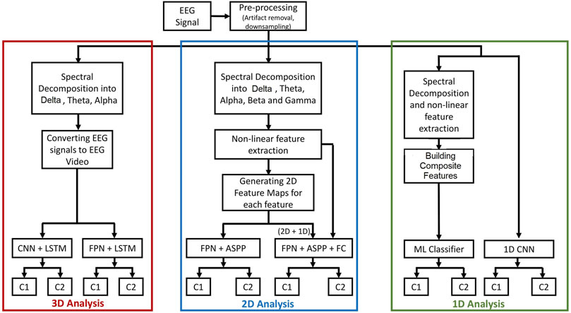
FIGURE 1. The proposed methodology for the analyzes of EEG using 1D, 2D, and 3D representations. In the 3D analysis, EEG signals are converted to videos and classified using: 1) the CNN and LSTM model or 2) the FPN and LSTM model. In the 2D analysis, feature maps are generated from hand-crafted features and classified using FPN and ASPP while a composite feature set consisting of 2D feature maps and 1D feature vector is classified using FPN and ASPP along with a fully connected classification layer. In the 1D analysis, 1D feature vectors are classified using traditional methods and raw EEG signals are analyzed using CNN.
Wavelet decomposition is widely used to decompose EEG signals into various sub-bands. Wavelet is a wave-like oscillation that is localized (compact in both time and frequency, used to analyse signals with minimum uncertainty in time–frequency simultaneously) in the time and frequency domains. In this work, 4-level decomposition with “db5” mother wavelet is used on the pre-processed EEG signals. Each of the levels of DWT results in approximation (A) and detail (D) coefficients which characterize the low and high frequency components, respectively. 4-Level decomposition used in this work is shown in Table 1.

TABLE 1. Frequency bands of EEG corresponding to the wavelet coefficients obtained from a 4-level wavelet decomposition of band-limited EEG.
Various features encapsulate multiple characteristics of EEG and therefore it is necessary to select the appropriate features which can extract relevant information from the EEG data for a given classification scenario. Commonly extracted features from EEG data can be broadly classified into three as: 1) Frequency domain—band power, Hurst exponent, differential entropy, and power spectral density, 2) Time domain—Peak-to-Peak, Hjorth parameters, fractal dimension, and higher order crossing, and 3) Spatial domain—magnitude squared coherence, rational asymmetry, and differential causality. After exhaustive analyses, the top five best performing features are selected and reported in this work. They are differential entropy, Hurst exponent, Hjorth activity, Hjorth complexity, and Hjorth mobility.
Differential entropy (DE) is used to measure the signal complexity in biomedical signals Chen et al. (2020) Zheng et al. (2018). For a Gaussian distribution, DE can be formulated as shown in Eq. 1
where X follows Gaussian distribution N (μ, σ2), π and e are constants, and x is a variable.
Hjorth activity parameter represents the average power of the signal (squared standard deviation of amplitude) and can be calculated as (Eq. 2)
where
Hjorth mobility parameter (HM) calculates the mean frequency of the signal or the standard deviation of the power spectrum and can be calculated as shown in Eq. 3
where x′ represents the derivative of the signal x.
Hjorth complexity parameter measures the change in frequency of the signal. It measures the deviation of the signal from a pure sine wave, and the values converge toward 1 if the signal is more similar to a pure sine wave. Hjorth complexity is calculated as (Eq. 4)
The Hurst exponent (H) is used to evaluate the absence or presence of long-range dependence in a time-series or to measure how much the signal deviates from a random walk. If the value of H is greater than 0.5, it indicates that the data has long-range correlations. Long-range anti-correlations are indicated by the H value less than 0.5, while H equals to 0.5 indicates random data. The equation to calculate Hurst exponent is given in Eq. 5
where R(n) is the range of the data series, S(n) is the sum of the standard deviation,
The pre-processed band-limited EEG signals are utilized to calculate various hand-crafted features. Discrete wavelet-transform is applied to decompose the EEG signals into five sub-bands—Delta (1–4 Hz), Theta (4–8 Hz), Alpha (8–14 Hz), Beta (14–32 Hz), and Gamma (32–64 Hz). The five hand-crafted features encapsulating various signal characteristics as mentioned in Section 2.2 are calculated for each of the five sub-bands and for each electrode. For each of the hand-crafted feature n × 5 a unit long 1-dimensional vector is generated, where n is the number of electrodes in each dataset.
n × 5 unit long feature vector is obtained separately for each of the hand-crafted features. Initially, each of these features is experimented individually to assess their effectiveness in classification. Each of the hand-crafted features (5 × number of channels) undergo the “SelectKBest” feature selection algorithm by Pedregosa et al. (2011) which computes chi-squared statistic and provides relevant scores. Multiple “k” values are experimented in this work, and it is found that k = 80 results in the peak performance across all datasets. Four different classification algorithms—k-NN, SVM, random forest (RF), and AdaBoost (AB) are utilized in this work. k-Nearest Neighbors (k-NN) is one of the commonly used classification algorithm. The main idea of the algorithm is to search for “k” neighbor subjects nearest to the unknown subject, and then classify the unknown subject based on majority votes of its “k” neighbors. Support vector machine (SVM) works by finding a hyperplane in an N-dimensional space that distinctly classifies the data points. The dimension of the hyperplane varies with the number of features. Random forest (RF) is based on the concept of ensemble learning. Decision trees are built on different samples and their majority vote is taken for classification. AdaBoost (AB) is another ensemble learning algorithm which first fits a classifier onto the original dataset, and then fits more copies of the same classifier but the weights of misclassified instances are adjusted to perform better.
A composite feature set is also experimented in this work to find the optimal combination of features and is shown in Figure 2. n × 5 unit long feature vector obtained for each of the hand-crafted features are concatenated to form a composite feature set. On the composite feature set, “SelectKBest” feature selection is carried out, and the resulting feature set is input to the four classifiers for classification.
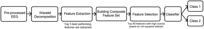
FIGURE 2. Analysis on 1D EEG representation with a composite feature set. The top performing features are found to be Hjorth parameters and differential entropy.
The pre-processed EEG can be utilized as the input without manual feature extraction to a 1D deep learning framework. This enables the model to extract those features that it deems effective for classification. Multi-layer 1D CNN is utilized here to perform data-driven feature extraction and classification. The base network architecture consists of two convolutions—batch normalization layers and one MaxPool layer, followed by another two convolutions—batch normalization layers and one MaxPool layer. The output from the last MaxPool layer is flattened and is input to a dense layer, followed by a final Softmax classification layer.
The five EEG sub-bands obtained by discrete wavelet decomposition as mentioned in Section 2.3.1 are utilized in this experiment. Since the EEG electrodes are placed on a scalp in a 3D space; in order to generate topography preserving 2D maps, the 3D location of the electrodes obtained using the standard 10/10 or 10/20 international system have to be converted to a 2D space. Additionally, it is imperative to preserve the relative distance between the electrodes in a 3D space when transforming to a 2D space Bashivan et al. (2015). In order to achieve this, polar projection, also known as Azimuthal Equidistant Projection (AEP), is utilized here Gao et al. (2020). Values calculated for each of the hand-crafted features for each of the sub-bands are placed at the transformed 2D location of the electrodes. Positions of the electrodes are mapped on to a 200, ×, 200 matrix. Delaunay Triangulation Interpolation technique is then applied to estimate the measurement values in-between the electrodes. This method of interpolation calculates the Delaunay triangulation between positions of the mapped electrodes Dimitrov (1998), to generate a smooth reconstructed spatial map with different activation regions and fine transitions between them. The two-dimensional feature maps are generated for each of the five sub-bands and are stacked forming 200 sized feature maps. The 2D feature maps care generated for each hand-crafted features individually.
A widely used deep learning framework, the convolution neural network (CNN), is utilized in this analysis. CNN comprises of a series of convolution layers, normalization layers, activation layers, pooling layers, and dropout layers. These layers which perform feature extraction on the input data are followed by multiple fully-connected layers for final classification. In this work, atrous spatial pyramid pooling (ASPP) and feature pyramid network (FPN) are utilized.
Multi-scale analysis widens the receptive field, providing context information at various scales. The ASPP module Benjdira et al. (2020) is utilized to perform the multi-scale analysis. The input is given to five convolution layers in parallel with 1, 2, 4, 6, and 12 dilation rates, respectively. Kernel size is set to 2 and the strides size is 1. The output from these five convolution layers are concatenated and input to a 1 × 1 convolution layer with kernel and stride size of 2. This forms a single ASPP module. Three such ASPP modules are utilized sequentially. In image classification, the feature pyramid network (FPN) has shown to boost the accuracy as observed in the study by Rahimzadeh et al. (2021). Hence, the FPN network is utilized in this work to boost the performance of the model. The complete network architecture is shown in Figure 3. The 3rd ASPP layer is upsampled and added with the output of the 2nd ASPP layer which had undergone the 1 × 1 convolution. This forms the first FPN layer. This process is repeated for FPN1 and the first ASPP layer resulting in FPN2. The MaxPool layer is applied to the outputs of FPN1, FPN2, and ASPP3, separately. The outputs from each MaxPool layers are flattened and concatenated, forming a single feature vector. The single feature vector is input to a fully connected layer, followed by the Softmax layer for classification.
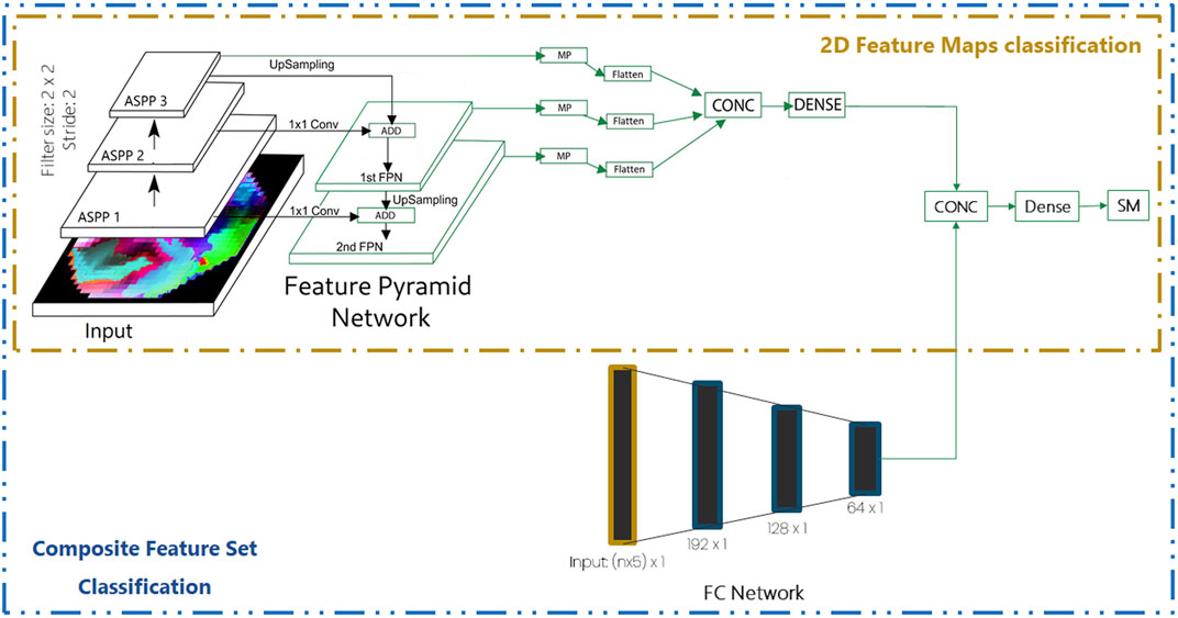
FIGURE 3. Network architecture for the analysis of 2D feature maps and a composite feature set consisting of 2D feature maps and 1D features. ASPP, atrous spatial pyramid pooling; FPN, feature pyramid network; MP, max pooling; CONC, concatenate; SM, softMax; n number of electrodes.
Another approach that utilizes the 2D feature map with 1D feature vector (n × 5 unit long feature vector) is also experimented here. As shown in Figure 3, the 2D feature maps undergo feature extraction as described in Section 2.4.2 and the output of the fully connected layer is utilized for concatenation with the output of the fully connected (FC) network. The fullyconnected (FC) network consists of multiple dense layers, as shown in Figure 3. The concatenated vector is input to a dense layer followed by the SoftMax layer for classification.
Roach and Mathalon, (2008) decomposed the pre-processed EEG signals into the magnitude and phase components (time–frequency analysis) using the method of spectral decomposition that utilized the fast Fourier transform (FFT). The process of using this method to obtain EEG sub-bands is known as frequency binning. In this experiment four EEG sub-bands, namely, Theta (4–7 Hz), Alpha (8–12 Hz), and Beta (12–40 Hz) obtained using frequency binning are utilized.
The proposed approach in this experiment utilizes topographical maps that preserve spatial information. As described in Section 2.4, electrodes placed on the scalp in a 3D space are converted to a 2D space using azimuthal equidistant projection (AEP) to preserve the relative distance between electrodes present in the 3D space. The three scalar values, obtained per time frame, through the method of frequency binning, for each electrode, are interpreted as channels of an image, which are then projected onto a 2D electrode location. To generate smooth topographical 2D maps, Delaunay triangulation interpolation is utilized. This interpolation algorithm estimates the spectral measurement values in-between the electrodes over a 32 × 32 grid. Smooth reconstructed spatial maps are generated with different activation regions having fine transitions between them. Such a sequence of these spatial maps, as shown in Figure 4, are stacked together in the time domain to create EEG videos. Videos are generated of the size t × m × m × c, where t is the length of the video, m is the spatial resolution of the video created using the grid, and c refers to the number of channels. The generated videos are passed to the video classification model as the input. The model utilizes spatial information using CNN and temporal information through RNN.
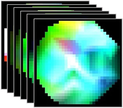
FIGURE 4. Sample of 6 contiguous frames of EEG video representation from the EEG Baseline dataset for the eyes open class.
CNN layers are utilized to exploit spatial and spectral information, whereas to exploit temporal information, LSTM is used. EEG videos are input to the multiple time-distributed convolution and MaxPool layers, followed by LSTM. The base network architecture has four convolutions—batch normalization layers and one MaxPool layer, followed by two convolutions—batch normalization and one MaxPool layers. This is further followed by one convolution - batch normalization and one MaxPool layers. The output of the last MaxPool layer is given in parallel to the LSTM and 1D temporal convolution layer. The outputs of LSTM and temporal convolution are concatenated and input to a dense layer of 256 dimensions, which is followed by the SoftMax layer. A kernel size of 3 and the “ReLU” activation function are used for the convolution layers. LSTM utilizes ‘tanh’ activation function. Time-distributed convolution and MaxPool layers are used in place of conventional CNN layers to utilize the EEG video as the input.
A conventional CNN model in combination with FPN (Feature Pyramid Network) are experimented in this work using the network architecture described in Section 2.5.2. The proposed FPN architecture is shown in Figure 5. The first layer of FPN (FPN1) is formed by adding the upsampled output of the 7th convolution layer with the output of 1 × 1 convolution of the output of 6th convolution layer. Similarly, the FPN2 layer is formed using outputs from FPN1 and the 5th convolution layer. The outputs of FPN1, FPN2, and the 7th convolution layer are inputs to three convolution and MaxPool layers in parallel. The outputs of each of the MaxPool layers are inputs to the LSTM and 1D temporal convolution in parallel. The outputs of all LSTM and 1D temporal convolution are concatenated and input to a dense layer followed by the SoftMax layer.
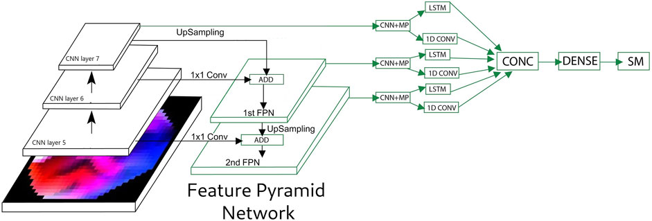
FIGURE 5. Feature pyramid network (FPN) and long–short term memory (LSTM) network for the EEG video. CNN, convolution neural network; MP, maxpool; CONC, concatenate; SM, softMax.
Binary cross-entropy loss along with the Adam optimizer is used for training for all the datasets. The scheduled learning rate is applied with a starting rate of 0.001. For EEG baseline and mental arithmetic, datasets are randomly split into train, test, and validation using stratified split and the model is trained seven times. 18% data are used for testing, 18% data are used for validation, and the rest 64% data are used for training the model. It is ensured that there is no data leakage between the splits. For the Parkinson’s disease dataset, 10 rounds of 10-fold cross validation are performed. Leave-one-subject-out method for evaluation is used for the emotion dataset. Different evaluation schemes are applied to different datasets for a comparison of the results with other works in the literature.
“EEG Motor/Movement Imagery” is a publicly available EEG dataset from Physionet PhysioBank, (2000) Schalk et al. (2004). Two distinct baseline runs available in the dataset are utilized in this work. The dataset contains EEG data consisting of 218 samples each of 1 min duration, sampled at 160 samples per second, from 109 volunteers. The two baseline runs are:
1. EEG recorded with open eyes
2. EEG recorded with closed eyes
The EEG signals were collected from 64 electrodes as per the international 10–10 system.
The EEG mental arithmetic dataset by Physionet PhysioBank, (2000) Zyma et al. (2019) consists of 72 one and 3 minute recordings from 36 patients before and during the performance of mental arithmetic tasks (two tasks), respectively. The EEG signals were recorded from 19 EEG-channels according to the international 10–20 system. The data were acquired at the sampling rate of 500 Hz. The subjects were asked to do an arithmetic task that involved the serial subtraction of two numbers. Each trial started with the communication of orally 4-digit (minuend) and 2- digit (subtrahend) numbers.
The publicly available dataset for Parkinson’s disease from the University of New Mexico (UNM) Anjum et al. (2020) is utilized in this work. EEGs were recorded from 27 PD patients and 27 controls. The control participants were matched for gender and age with the PD patients. EEG signals were recorded with subjects at the rest state. The data were captured under both the resting conditions of eyes-open and eyes-closed. 64 Ag/AgCl electrodes were used to collect the data at a sampling rate of 500 Hz across 0.1–100 Hz using the Brain Vision system. A reference channel was set to CPz.
SJTU emotion EEG dataset (SEED) Zheng and Lu, (2015) is utilized in this work for emotion classification. It contains EEG signals and eye movement signals from 15 participants (7 males and 8 females, and aged 23.27 ± 2.37). The data were collected via 62 electrodes while the participants were watching fifteen Chinese film clips with three types of emotions, i.e., negative, positive, and neutral. With an interval of about 1 week, three experiments were performed for each participant. The EEG data, recorded for approximately 4 minutes per trial, were down-sampled to 200 Hz. A band-pass filter from 0 to 75 Hz was applied. In the present study, only positive and negative trials from the participants are used.
The efficacy of various multi-dimensional representations of EEG data as 1D—feature vector, 2D—feature map, and 3D—video, for the purpose of classification in diverse scenarios as described in Section 3, are explored in this work.
As described in Section 2.3.2, hand-crafted features are calculated and n × 5 unit long vector is generated where n is the number of electrodes and 5 indicates the number of sub-bands. The five features are input to four classifiers for classification. Results of this method on the four datasets are presented in Table 2. It is seen from Table 2 that for the EEG baseline classification, a peak mean accuracy of 88.28% is achieved using the optimal feature–classifier combination of Hjorth mobility and the random forest model. 76.67% peak mean accuracy is attained on the mental arithmetic dataset using differential entropy and SVM, while Hjorth complexity in combination with SVM results in 82.22% peak mean performance for the Parkinson’s disease dataset. Individually, Hurst exponent and Hjorth mobility result in a peak mean performance of 73.77% in classifying positive and negative emotions.
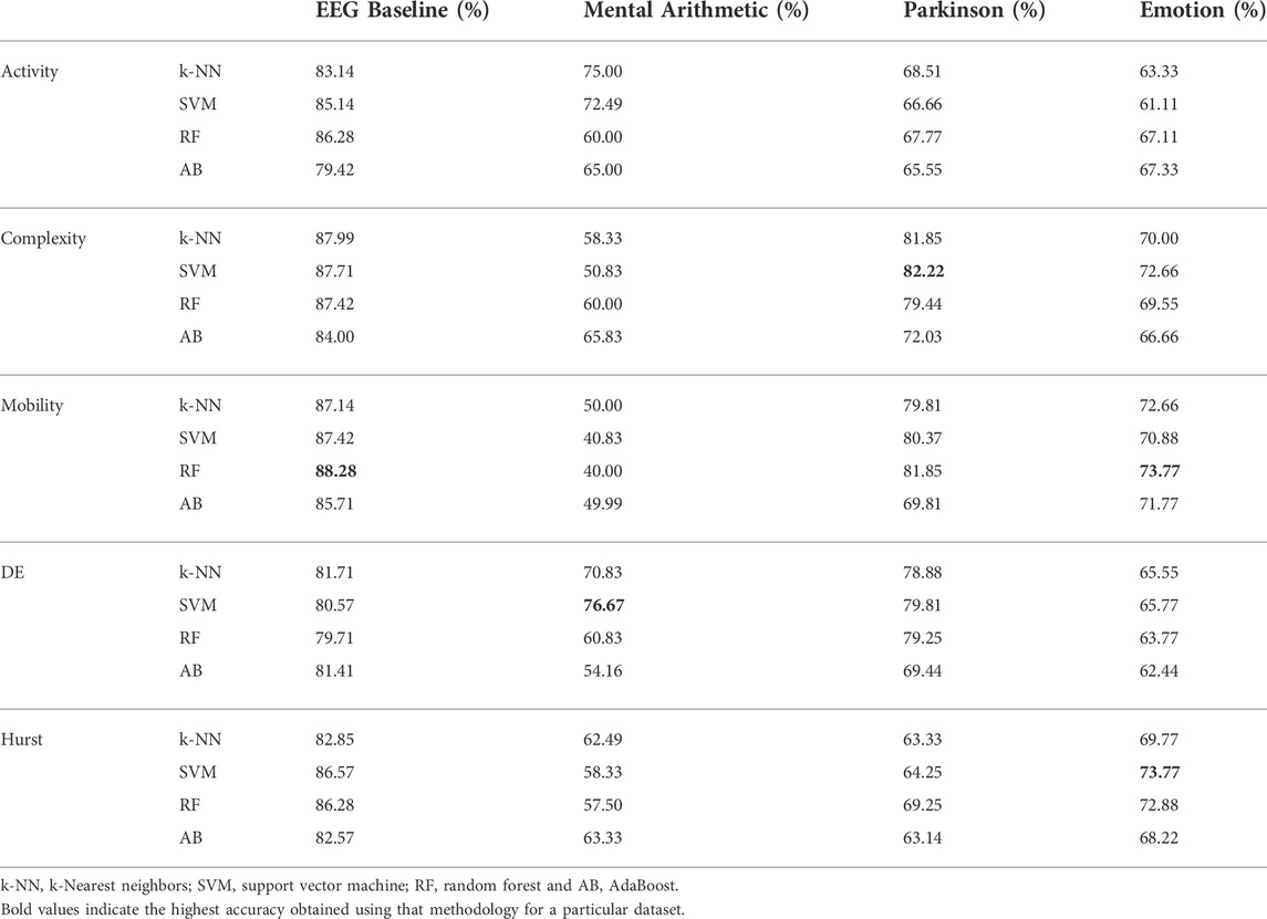
TABLE 2. Mean accuracies obtained for 1D non-linear feature vectors trained using traditional methods.
A composite feature set is experimented for various combinations of the hand-crafted features using the methodology as shown in Figure 2. It is observed that the combination of Hjorth—activity, Hjorth—mobility, Hjorth—complexity, and differential entropy results in the optimal performance. Table 3 shows the results of the composite feature set for various classifiers and datasets. As can be observed from the table, the composite feature set results in the peak mean performances of 88.56% (higher by 0.32%), 83.33% (higher by 7%), 88.51% (higher by 6%), and 70.66% (lower by 3%) for EEG baselines, mental arithmetic, Parkinson’s disease, and emotion datasets, respectively.
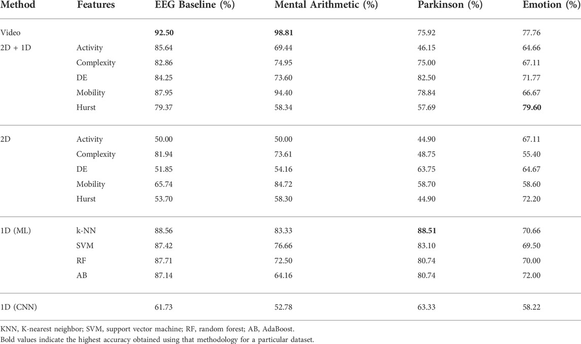
TABLE 3. Mean accuracies obtained using the proposed methodologies on the mentioned datasets.
EEG signals are given as the input to CNN as explained in Section 2.3.3 to exploit data-driven feature representation and classification characteristics of deep learning. As observed from Table 3, this method results in peak mean performances of 61.73%, 52.78%, 63.33%, and 58.22% for EEG baselines, mental arithmetic, Parkinson’s disease, and emotion datasets, respectively. The performances are observed to be lower than the aforementioned hand-crafted features. It must be noted that the EEG signals are not frequency decomposed into sub-bands before being inputted to the CNN. To utilize a completely data-driven approach, no sub-band decomposition is used in this methodology.
The 2D analysis as described in Section 2.4.2 is carried out to retain the spatial structure of the electrodes’ positions and a 2D feature maps’ classification module as shown in Figure 3 is used. It is observed from Table 3 that the 2D feature map generated using Hjorth complexity distinguishes the EEG baselines, with a peak mean performance of 81.94%, while Hjorth mobility results in a peak mean accuracy of 84.72% for mental arithmetic. In the scenarios involving Parkinson’s disease and emotion datasets, differential entropy and Hurst feature maps result in 63.75% and 72.2% peak mean accuracies, respectively.
A composite feature set of 2D feature maps along with 1D features is also explored, as shown in Figure 3. A combination of Hjorth mobility 2D feature maps with Hjorth mobility 1D features results in a peak mean performance of 87.95% for EEG baselines. This performance is 6% higher than the method using only 2D feature maps. Similarly, the same feature combination results in a peak performance of 94.4% for mental arithmetic, which is 10% higher than using only 2D feature maps. The trend follows for both Parkinson’s disease and emotion datasets where composite features of differential entropy and the composite features of Hurst exponent result in peak mean accuracies of 82.5% and 79.6%, respectively. This is 18.75% and 7.4% higher than using only 2D feature maps. The results clearly show that the composite feature set consisting of 2D feature maps with corresponding 1D features surpass the performance of using only 2D feature maps from a minimum accuracy of 6% to a maximum accuracy of 18.75%.
To simultaneously exploit temporal, spectral, and spatial information, EEG signals are converted into EEG videos as mentioned in Section 2.5.1. Time-distributed convolution layers are utilized to preserve temporal information, which is subsequently utilized by LSTM. A combination of the CNN–RNN Bashivan et al. (2015) network as explained in Section 2.5.2 is explored. This method resulted in a peak mean accuracy of 86.9%. When dropout is introduced in the network to avoid the issue of over-fitting, it reduces the performance by 9% resulting in a peak mean accuracy of 77.8%. l2-regularization is introduced as an alternative to dropout, which boosts the performance to 92.5%. Hence, l2-regularization is utilized in all methodologies involving EEG video inputs across datasets; this results in peak mean accuracies of 96.64%, 73.6%, and 69.5% for mental arithmetic, Parkinson’s disease, and emotion datasets, respectively.
A modified architecture involving the feature pyramid network (FPN) as shown in Figure 5 is also explored. Introduction of FPN decreases the performance of EEG baselines by 2.5% but improves the performance of the network in the other three datasets. Peak mean accuracies of 98.81%, 75.92%, and 74.36% are obtained for mental arithmetic, Parkinson’s disease, and emotion datasets, respectively.
A comparison of the performances of the proposed methodologies with other works in the literature is shown in Table 4. The analysis of the 3D representation of EEG as videos yield 3.27% and 2.9% higher performances than the state-of-the-art for EEG baselines and mental arithmetic, respectively. For the Parkinson’s disease dataset, a 3.11% higher accuracy than the state-of-the art is achieved using traditional methods involving composite features for 1D representation of EEG while the composite features consisting of 2D feature maps and 1D features of differential entropy result in 3% less performance than the state-of-the art. A peak mean performance of 79.60% is obtained using the composite feature set consisting of 2D feature maps and 1D features of the Hurst exponent for emotion dataset; however, this performance is 8.85% less than the state-of-the-art.
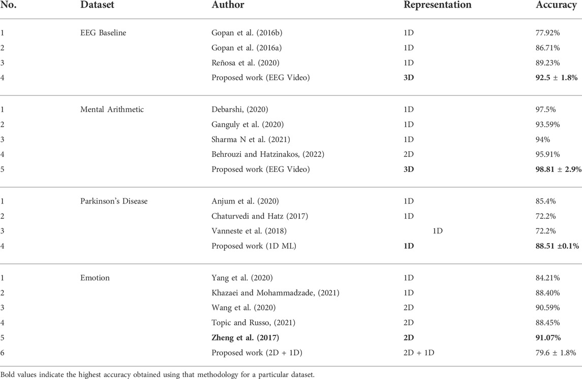
TABLE 4. Comparison of the accuracy achieved using the proposed methodologies with other works in the literature.
Confusion matrices for the methods resulting in peak mean performances for each of the dataset are shown in Figure 6. It can be observed that 10% of the eyes open baseline is misclassified as eyes closed, whereas only 5% of eyes closed is misclassified as eyes Open. In the case of mental arithmetic, the only misclassification is the cognitive state as a state of rest, which is approximately 2.4%. In the Parkinson’s disease analysis, it is observed that the Type 1 error (14.82%) is higher than the Type 2 error (8.15%). In emotion classification, the same extent of misclassification (20%) is observed for both the classes.
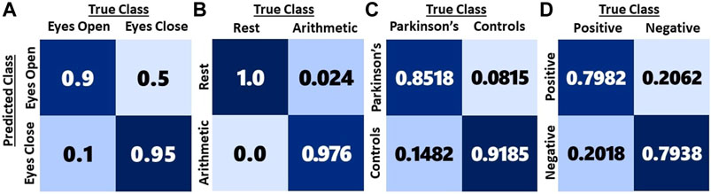
FIGURE 6. Confusion matrices of high performing multi-dimensional EEG representations for the four datasets. (A) EEG baseline dataset using the EEG video. (B) Mental Arithmetic dataset using the EEG video. (C) Parkinson’s disease dataset using 1D features. (D) Emotion dataset using the composite feature set consisting of 2D feature maps and 1D features.
In this work, three distinct multi-dimensional representations of EEG data, namely, 1D (feature vector and raw signals), 2D (feature maps), and 3D (EEG videos) are analyzed on data corresponding to four diverse classification scenarios. In the methodologies involving 1D representation, on one hand, we extract hand-crafted features using traditional methods; on the other hand, a data-driven framework such as 1D CNN, which uses raw EEG signals as the input, is explored. 2D Feature maps generated using hand-crafted features are utilized in a deep learning classification framework, and a combination of 2D feature maps with 1D features is also explored. 3D representation of EEG data is analyzed using a combination of CNN and RNN networks as well as with the use of FPN.
In the case of 1D representation of EEG signals, the characteristic changes in hand-crafted features for the EEG sub-bands are considered with the limitation that the spatial information cannot be incorporated. The composite feature set of Hjorth parameters - activity, mobility, complexity, and differential entropy result in higher performances for three of the classification scenarios. 2D feature map-based analyses utilize the non-linear characteristics of the brain waves at various electrode positions by preserving spatial information. The Hjorth activity feature map measures the average power of the brain regions in comparison with other brain regions. The Hjorth mobility feature map captures the deviation in the power spectrum of different brain regions. The Hjorth complexity feature map provides a measure of similarity of EEG signals at different brain regions to a pure sine wave. The long-range dependencies of EEG signals of different brain regions and the changes in the signal complexity of brain regions are captured by Hurst exponent and differential entropy feature maps, respectively. However, it is observed that the composite feature set consisting of 2D feature maps and 1D features of the same handcrafted features result in a higher performance than using the 2D feature map alone. This could be because the composite feature set exploits the spatial information from 2D feature maps as well as the characteristic changes in the hand-crafted features using 1D features. The EEG video analyses utilize spatial, spectral, and temporal information simultaneously and exploit the topographical changes in the brain activation regions.
In view of these choices of multi-dimensional EEG representations, the following inferences can be concluded based on the analyses on the four diverse datasets. During the eyes open and eyes closed baselines, studies Barry et al. (2007) observed topographical and power level changes in the brain activations. During the eyes open baseline, the prefrontal cortex (PF) and the frontopolar cortex (FPC) regions were observed to have higher levels of power as compared to eyes closed. Significant changes in the occipital and parietal lobes were also observed during these states in Kan et al. (2017). Thus, an analysis based on EEG video representation is able to exploit the inherent characteristic differences between the EEG baselines. Changes in the mean frequencies across various brain regions are utilized using the composite feature set of Hjorth mobility to distinguish the baselines. The overall changes in the power levels of brain activations are exploited by the 1D EEG representation using hand-crafted features, leading to a higher performance. In the case of mental arithmetic, Abd Hamid et al. (2011) observed activations in the brain regions of the frontal and parietal lobes while performing the tasks of addition and subtraction. These two regions are known to be involved during mental calculationZago et al. (2001). It was observed by Arsalidou et al. (2018) that the superior frontal and medial frontal brain regions were also the key regions for calculations and working memory. Hence, the analysis based on EEG video representation utilizes the topographical changes in brain activation regions during the cognitive state and the state of rest to distinguish between the two classes. The changes in the mean frequencies across brain regions as well as the overall changes in brain activations are exploited in the analyses involving 2D EEG and 1D EEG representations.
The topographical changes along with the spectral and temporal information need to be consistent across subjects for a particular class to effectively use the analysis based on EEG video representation. The degree of deterioration of brain regions and the effect of such degradation on the brain activation regions need not necessarily be consistent for all subjects suffering from Parkinson’s disease. This inconsistency could be the reason why the analysis based on EEG video representation resulted in a peak mean performance of only 75.9% (13% less than the peak performance obtained using the 1D feature vector analysis). The varying degrees of deterioration of brain regions in Parkinson’s disease result in characteristic changes in the EEG signals of various brain regions. This includes changes in the signal complexity of the brain regions, which is well utilized by differential entropy to distinguish subjects with Parkinson’s disease from healthy controls. These regions may not be consistent, and hence the incorporation of spatial information into the analyses might not be effective. This is illustrated on the Parkinson’s disease dataset when the performance of the analysis based on EEG 1D feature vector representation is compared with that involving the 2D feature map and EEG video representation.
Multiple regions in the brain are involved during positive and negative emotionsVytal and Hamann (2010). Though there were no specific visible patterns of topographical changes associated with the positive and negative emotions, the study by Lindquist et al. (2016) found that the activations have higher power levels during negative emotions as compared to positive emotions. This could be the reason for the peak mean performance of 77.76% with the analysis based on EEG video representation indicating the potential of the proposed approach with different network architectures, even though currently, the performance is approximately 11% less than the state-of-the-art. Though the topographical changes associated with positive and negative emotions are similar, the Hurst exponent distinguished the two types of emotions, with high performance indicating significant changes in the long-range dependencies of EEG signals of different brain regions.
The study shows that, while 3D-video representation of EEG signals encompasses rich information, this methodology proves useful only when there are significant topographical changes in brain activations and the changes are consistent for a particular class. Apart from this, the efficacy of this representation is high when spectral and temporal changes, across the classes, are significant. 2D-feature map representation is important when spatial information is combined with either spectral or temporal information, but not all three simultaneously. 1D-feature vector representations are useful in cases where spatial information is not critical. Thus, the choice of the EEG data representation and analyses depends on the type of classification scenario being considered and the characteristics of the EEG signals of the considered classes that can be exploited.
The efficacies of various multi-dimensional representations of EEG signals are analyzed in this work for diverse classification scenarios. EEG data are represented in terms of 1D–feature vector, 2D–feature maps, and 3D—EEG videos. 1D hand-crafted features were analyzed using traditional methods and 1D signals were analyzed using 1D CNN. 2D feature maps and a composite feature set of 2D feature maps along with 1D features were proposed and explored using deep learning frameworks. Furthermore, EEG videos were analyzed using a combination of temporal convolution and LSTM. An architecture involving the feature pyramid network (FPN) and atrous spatial pyramid pooling (ASPP) is proposed for 2D feature maps and EEG video analyses. Four diverse datasets - EEG baseline, EEG mental arithmetic, Parkinson’s disease, and emotion datasets are analyzed using the proposed EEG representations and networks. The Analysis of EEG video representation resulted in peak mean performances of 3.27% and 2.9% higher than the state-of-the-art for EEG baselines and mental arithmetic, respectively. 1D EEG representation with traditional methods resulted in 3.11% higher accuracy than the state-of-the art for Parkinson’s disease. From the study, it can be inferred that the EEG can be analyzed using various multi-dimensional representations. However, the representation needs to be chosen based on the classification scenarios being considered and whether spatial, spectral, and temporal information need to be exploited simultaneously or in various combinations.
Publicly available datasets were analyzed in this study. These data can be found here: 1) EEG Baseline dataset from Physionet: https://physionet.org/content/eegmmidb/1.0.0/ 2) Mental Arithmetic dataset from Physionet: https://physionet.org/content/eegmat/1.0.0/ 3) Parkinson’s disease dataset from Narayanan Labs: https://bit.ly/Anjum2020 4) Emotion dataset by SEED: https://bcmi.sjtu.edu.cn/home/seed/seed.html
Ethical review and approval was not required for the study on human participants in accordance with the local legislation and institutional requirements. The patients/participants provided their written informed consent to participate in this study.
DS and GGK contributed in conceptualization, investigation, and in the development of the methodology. DS carried out the implementation and wrote the first draft. GGK and NS supervised the work and were involved in writing–reviewing–editing. NS validated the work and provided the resources.
This work was funded by Machine Intelligence and Robotics Center (MINRO) Project GoK, IIITB. It is supported by Karnataka Innovation and Technology Society, Department of IT, BT and S&T, Govt. of Karnataka vide GO No. ITD 76 ADM 2017, Bengaluru; Dated 28.02.2018.
The authors declare that the research was conducted in the absence of any commercial or financial relationships that could be construed as a potential conflict of interest.
All claims expressed in this article are solely those of the authors and do not necessarily represent those of their affiliated organizations, or those of the publisher, the editors, and the reviewers. Any product that may be evaluated in this article, or claim that may be made by its manufacturer, is not guaranteed or endorsed by the publisher.
Abd Hamid, A. I., Yusoff, A. N., Mukari, S. Z.-M. S., and Mohamad, M. (2011). Brain activation during addition and subtraction tasks in-noise and in-quiet. Malays. J. Med. Sci. 18, 3–15.
Anjum, M. F., Dasgupta, S., Mudumbai, R., Singh, A., Cavanagh, J. F., and Narayanan, N. S. (2020). Linear predictive coding distinguishes spectral eeg features of Parkinson’s disease. Park. Relat. Disord. 79, 79–85. doi:10.1016/j.parkreldis.2020.08.001
Arsalidou, M., Pawliw-Levac, M., Sadeghi, M., and Pascual-Leone, J. (2018). Brain areas associated with numbers and calculations in children: Meta-analyses of fmri studies. Dev. Cogn. Neurosci. 30, 239–250. doi:10.1016/j.dcn.2017.08.002
Barry, R. J., Clarke, A. R., Johnstone, S. J., Magee, C. A., and Rushby, J. A. (2007). Eeg differences between eyes-closed and eyes-open resting conditions. Clin. Neurophysiol. 118, 2765–2773. doi:10.1016/j.clinph.2007.07.028
Bashivan, P., Rish, I., Yeasin, M., and Codella, N. (2015). Learning representations from eeg with deep recurrent-convolutional neural networks. in ICLR 2016, November 19, 2015. arXiv preprint arXiv:1511.06448. doi:10.48550/arXiv.1511.06448
Behrouzi, T., and Hatzinakos, D. (2022). Graph variational auto-encoder for deriving eeg-based graph embedding. Pattern Recognit. 121, 108202. doi:10.1016/j.patcog.2021.108202
Benjdira, B., Ouni, K., Al Rahhal, M. M., Albakr, A., Al-Habib, A., Mahrous, E., et al. (2020). Spinal cord segmentation in ultrasound medical imagery. Appl. Sci. 10, 1370. doi:10.3390/app10041370
Bi, X., and Wang, H. (2019). Early alzheimer’s disease diagnosis based on eeg spectral images using deep learning. Neural Netw. 114, 119–135. doi:10.1016/j.neunet.2019.02.005
Chaturvedi, M., and Hatz, F. (2017). Quantitative EEG (QEEG) measures differentiate Parkinson's disease (PD) patients from healthy controls (HC). Front. Aging Neurosci. 9, 3. doi:10.3389/fnagi.2017.00003
Chen, G., Zhang, X., Sun, Y., and Zhang, J. (2020). Emotion feature analysis and recognition based on reconstructed eeg sources. IEEE Access 8, 11907–11916. doi:10.1109/access.2020.2966144
Cheng, J., Chen, M., Li, C., Liu, Y., Song, R., Liu, A., et al. (2020). Emotion recognition from multi-channel eeg via deep forest. IEEE J. Biomed. Health Inf. 25, 453–464. doi:10.1109/jbhi.2020.2995767
Debarshi, N. (2020). Eeg-based mental workload detection in a mental arithmetic task using machine learning. Int. J. Adv. Sci. Technol. 29, 13975–13984. http://sersc.org/journals/index.php/IJAST/article/view/33199.
Dimitrov, L. I. (1998). Texturing 3d-reconstructions of the human brain with eeg-activity maps. Hum. brain Mapp. 6, 189–202. doi:10.1002/(sici)1097-0193(1998)6:4<189::aid-hbm1>3.0.co;2-#
Fernández, T., Harmony, T., Rodríguez, M., Bernal, J., Silva, J., Reyes, A., et al. (1995). Eeg activation patterns during the performance of tasks involving different components of mental calculation. Electroencephalogr. Clin. neurophysiology 94, 175–182. doi:10.1016/0013-4694(94)00262-j
Ganguly, B., Chatterjee, A., Mehdi, W., Sharma, S., and Garai, S. (2020). “Eeg based mental arithmetic task classification using a stacked long short term memory network for brain-computer interfacing,” in 2020 IEEE Vlsi Device Circuit And System (Vlsi Dcs) (IEEE), 89–94.
Gao, Y., Gao, B., Chen, Q., Liu, J., and Zhang, Y. (2020). Deep convolutional neural network-based epileptic electroencephalogram (eeg) signal classification. Front. Neurol. 11, 375. doi:10.3389/fneur.2020.00375
Gonzalez, H. A., Yoo, J., and Elfadel, I. M. (2019). “Eeg-based emotion detection using unsupervised transfer learning,” in 2019 41st Annual International Conference of the IEEE Engineering in Medicine and Biology Society (EMBC) (IEEE), 694.
Gopan, K. G., Prabhu, S. S., and Sinha, N. (2020). Sleep eeg analysis utilizing inter-channel covariance matrices. Biocybern. Biomed. Eng. 40, 527–545. doi:10.1016/j.bbe.2020.01.013
Gopan, K. G., Reddy, S. A., Rao, M., Sinha, N., et al. (2022). Analysis of single channel electroencephalographic signals for visual creativity: A pilot study. Biomed. Signal Process. Control 75, 103542. doi:10.1016/j.bspc.2022.103542
Gopan, K. G., Sinha, N., and Babu J, D. (2016a). “Distribution based eeg baseline classification,” in International Conference on Computer Vision, Graphics, and Image processing, 314–321.
Gopan, K. G., Sinha, N., and Babu J, D. (2016b). “Statistical feature analysis for eeg baseline classification: Eyes open vs eyes closed,” in 2016 IEEE Region 10 Conference (TENCON), 2466. doi:10.1109/TENCON.2016.7848476
Ieracitano, C., Mammone, N., Bramanti, A., Hussain, A., and Morabito, F. C. (2019). A convolutional neural network approach for classification of dementia stages based on 2d-spectral representation of eeg recordings. Neurocomputing 323, 96–107. doi:10.1016/j.neucom.2018.09.071
Ieracitano, C., Mammone, N., Hussain, A., and Morabito, F. C. (2020). A novel multi-modal machine learning based approach for automatic classification of eeg recordings in dementia. Neural Netw. 123, 176–190. doi:10.1016/j.neunet.2019.12.006
Jiang, D., Lu, Y.-n., Yu, M., and Yuanyuan, W. (2019). Robust sleep stage classification with single-channel eeg signals using multimodal decomposition and hmm-based refinement. Expert Syst. Appl. 121, 188–203. doi:10.1016/j.eswa.2018.12.023
Kan, D., Croarkin, P. E., Phang, C., and Lee, P. (2017). Eeg differences between eyes-closed and eyes-open conditions at the resting stage for euthymic participants. Neurophysiology 49, 432–440. doi:10.1007/s11062-018-9706-6
Khazaei, E., and Mohammadzade, H. (2021). Temporal analysis of functional brain connectivity for eeg-based emotion recognition. arXiv preprint arXiv:2112.12380. doi:10.48550/arXiv.2112.12380
Kwak, Y., Kong, K., Song, W.-J., Min, B.-K., and Kim, S.-E. (2020). Multilevel feature fusion with 3d convolutional neural network for eeg-based workload estimation. IEEE Access 8, 16009–16021. doi:10.1109/access.2020.2966834
Lindquist, K. A., Satpute, A. B., Wager, T. D., Weber, J., and Barrett, L. F. (2016). The brain basis of positive and negative affect: Evidence from a meta-analysis of the human neuroimaging literature. Cereb. Cortex 26, 1910–1922. doi:10.1093/cercor/bhv001
Meng, J., Zhang, S., Beyko, A., Olsoe, J., Baxter, B., He, B., et al. (2020). Author correction: Noninvasive electroencephalogram based control of a robotic arm for reach and grasp tasks. Sci. Rep. 10, 6627. doi:10.1038/s41598-020-63070-z
Murugappan, M., Alshuaib, W. B., Bourisly, A., Sruthi, S., Khairunizam, W., Shalini, B., et al. (2020). “Emotion classification in Parkinson’s disease eeg using rqa and elm,” in 2020 16th IEEE International Colloquium on Signal Processing & Its Applications (CSPA) (IEEE), 290.
Oh, S. L., Hagiwara, Y., Raghavendra, U., Yuvaraj, R., Arunkumar, N., Murugappan, M., et al. (2020). A deep learning approach for Parkinson’s disease diagnosis from eeg signals. Neural comput. Appl. 32, 10927–10933. doi:10.1007/s00521-018-3689-5
Pedregosa, F., Varoquaux, G., Gramfort, A., Michel, V., Thirion, B., Grisel, O., et al. (2011). Scikit-learn: Machine learning in Python. J. Mach. Learn. Res. 12, 2825–2830. https://www.jmlr.org/papers/v12/pedregosa11a.html.
PhysioBank, P. (2000). Physionet: Components of a new research resource for complex physiologic signals. Circulation 101, e215–e220. doi:10.1161/01.cir.101.23.e215
Qureshi, M. B., Afzaal, M., Qureshi, M. S., Fayaz, M., et al. (2021). Machine learning-based eeg signals classification model for epileptic seizure detection. Multimed. Tools Appl. 80, 17849–17877. doi:10.1007/s11042-021-10597-6
Raghu, S., Sriraam, N., Vasudeva Rao, S., Hegde, A. S., and Kubben, P. L. (2020). Automated detection of epileptic seizures using successive decomposition index and support vector machine classifier in long-term eeg. Neural comput. Appl. 32, 8965–8984. doi:10.1007/s00521-019-04389-1
Rahimzadeh, M., Attar, A., and Sakhaei, S. M. (2021). A fully automated deep learning-based network for detecting Covid-19 from a new and large lung ct scan dataset. Biomed. Signal Process. Control 68, 102588. doi:10.1016/j.bspc.2021.102588
Reñosa, C. R. M., Sybingco, E., Vicerra, R. R. P., and Bandala, A. A. (2020). Eye state classification through analysis of eeg data using deep learning. In 2020 IEEE 12th International Conference on Humanoid, Nanotechnology, Information Technology, Communication and Control, Environment, and Management (HNICEM). doi:doi:10.1109/HNICEM51456.2020.9400081
Roach, B. J., and Mathalon, D. H. (2008). Event-related eeg time-frequency analysis: An overview of measures and an analysis of early gamma band phase locking in schizophrenia. Schizophr. Bull. 34, 907–926. doi:10.1093/schbul/sbn093
Rodrigues, J. d. C., Rebouças Filho, P. P., Peixoto, E., Kumar, A., and de Albuquerque, V. H. C. (2019). Classification of eeg signals to detect alcoholism using machine learning techniques. Pattern Recognit. Lett. 125, 140–149. doi:10.1016/j.patrec.2019.04.019
Roslan, N. S., Izhar, L. I., Faye, I., Saad, M. N. M., Sivapalan, S., Rahman, M. A., et al. (2017). Review of eeg and erp studies of extraversion personality for baseline and cognitive tasks. Personality Individ. Differ. 119, 323–332. doi:10.1016/j.paid.2017.07.040
Ruffini, G., Ibañez, D., Castellano, M., Dubreuil-Vall, L., Soria-Frisch, A., Postuma, R., et al. (2019). Deep learning with eeg spectrograms in rapid eye movement behavior disorder. Front. Neurol. 10, 806. doi:10.3389/fneur.2019.00806
Sadiq, M. T., Yu, X., Yuan, Z., Fan, Z., Rehman, A. U., Li, G., et al. (2019). Motor imagery eeg signals classification based on mode amplitude and frequency components using empirical wavelet transform. Ieee Access 7, 127678–127692. doi:10.1109/access.2019.2939623
Saikia, A., Hussain, M., Barua, A. R., Paul, S., et al. Department of Biomedical Engineering, North-Eastern Hill University, Shillong, IndiaDepartment of Neurology, North Eastern Indira. Gandhi Regional Institute of Health and Medical Science, Shillong, India. (2019). Eeg-emg correlation for Parkinson’s disease. Int. J. Eng. Adv. Technol. 8, 1179–1185. doi:10.35940/ijeat.f8360.088619
Schalk, G., McFarland, D. J., Hinterberger, T., Birbaumer, N., and Wolpaw, J. R. (2004). Bci2000: A general-purpose brain-computer interface (bci) system. IEEE Trans. Biomed. Eng. 51, 1034–1043. doi:10.1109/tbme.2004.827072
Sharma, L. D., Saraswat, R. K., and Sunkaria, R. K. (2021). Cognitive performance detection using entropy-based features and lead-specific approach. Signal Image Video process. 15, 1821–1828. doi:10.1007/s11760-021-01927-0
Sharma, N., Kolekar, M. H., and Jha, K. (2021). Eeg based dementia diagnosis using multi-class support vector machine with motor speed cognitive test. Biomed. Signal Process. Control 63, 102102. doi:10.1016/j.bspc.2020.102102
Shi, X., Wang, T., Wang, L., Liu, H., and Yan, N. (2019). “Hybrid convolutional recurrent neural networks outperform cnn and rnn in task-state eeg detection for Parkinson’s disease,” in 2019 Asia-Pacific Signal and Information Processing Association Annual Summit and Conference (APSIPA ASC) (IEEE), 939.
Tan, B., Kong, X., Yang, P., Jin, Z., and Li, L. (2013). The difference of brain functional connectivity between eyes-closed and eyes-open using graph theoretical analysis. Comput. Math. methods Med. 2013, 976365. doi:10.1155/2013/976365
Topic, A., and Russo, M. (2021). Emotion recognition based on eeg feature maps through deep learning network. Eng. Sci. Technol. Int. J. 24, 1442–1454. doi:10.1016/j.jestch.2021.03.012
Torres, E. P., Torres, E. A., Hernández-Álvarez, M., and Yoo, S. G. (2020). Emotion recognition related to stock trading using machine learning algorithms with feature selection. IEEE Access 8, 199719–199732. doi:10.1109/ACCESS.2020.3035539
Vanneste, S., Song, J.-J., and De Ridder, D. (2018). Thalamocortical dysrhythmia detected by machine learning. Nat. Commun. 9, 1103. doi:10.1038/s41467-018-02820-0
Vaughan, T. M. (2020). Brain-computer interfaces for people with amyotrophic lateral sclerosis. Handb. Clin. Neurol. 168, 33–38. doi:10.1016/B978-0-444-63934-9.00004-4
Vytal, K., and Hamann, S. (2010). Neuroimaging support for discrete neural correlates of basic emotions: A voxel-based meta-analysis. J. cognitive Neurosci. 22, 2864–2885. doi:10.1162/jocn.2009.21366
Wang, F., Wu, S., Zhang, W., Xu, Z., Zhang, Y., Wu, C., et al. (2020). Emotion recognition with convolutional neural network and eeg-based efdms. Neuropsychologia 146, 107506. doi:10.1016/j.neuropsychologia.2020.107506
Yang, J., Huang, X., Wu, H., and Yang, X. (2020). Eeg-based emotion classification based on bidirectional long short-term memory network. Procedia Comput. Sci. 174, 491–504. doi:10.1016/j.procs.2020.06.117
Zago, L., Pesenti, M., Mellet, E., Crivello, F., Mazoyer, B., Tzourio-Mazoyer, N., et al. (2001). Neural correlates of simple and complex mental calculation. Neuroimage 13, 314–327. doi:10.1006/nimg.2000.0697
Zhang, P., Wang, X., Zhang, W., and Chen, J. (2018). Learning spatial–spectral–temporal eeg features with recurrent 3d convolutional neural networks for cross-task mental workload assessment. IEEE Trans. Neural Syst. Rehabil. Eng. 27, 31–42. doi:10.1109/tnsre.2018.2884641
Zheng, W.-L., Liu, W., Lu, Y., Lu, B.-L., and Cichocki, A. (2018). Emotionmeter: A multimodal framework for recognizing human emotions. IEEE Trans. Cybern. 49, 1110–1122. doi:10.1109/tcyb.2018.2797176
Zheng, W.-L., and Lu, B.-L. (2015). Investigating critical frequency bands and channels for eeg-based emotion recognition with deep neural networks. IEEE Trans. Auton. Ment. Dev. 7, 162–175. doi:10.1109/tamd.2015.2431497
Zheng, W.-L., Zhu, J.-Y., and Lu, B.-L. (2017). Identifying stable patterns over time for emotion recognition from eeg. IEEE Trans. Affect. Comput. 10, 417–429. doi:10.1109/taffc.2017.2712143
Keywords: EEG, multi-dimensional representations, deep learning, classification, feature pyramid network (FPN), convolution neural network (CNN), EEG video
Citation: Shah D, Gopan K. G and Sinha N (2022) An investigation of the multi-dimensional (1D vs. 2D vs. 3D) analyses of EEG signals using traditional methods and deep learning-based methods. Front. Sig. Proc. 2:936790. doi: 10.3389/frsip.2022.936790
Received: 05 May 2022; Accepted: 27 June 2022;
Published: 25 July 2022.
Edited by:
Mahesh Raveendranatha Panicker, Indian Institute of Technology Palakkad, IndiaReviewed by:
Juan Cheng, Hefei University of Technology, ChinaCopyright © 2022 Shah, Gopan K. and Sinha. This is an open-access article distributed under the terms of the Creative Commons Attribution License (CC BY). The use, distribution or reproduction in other forums is permitted, provided the original author(s) and the copyright owner(s) are credited and that the original publication in this journal is cited, in accordance with accepted academic practice. No use, distribution or reproduction is permitted which does not comply with these terms.
*Correspondence: Gopika Gopan K., Z29waWthLmdvcGFua0BpaWl0Yi5hYy5pbg==
Disclaimer: All claims expressed in this article are solely those of the authors and do not necessarily represent those of their affiliated organizations, or those of the publisher, the editors and the reviewers. Any product that may be evaluated in this article or claim that may be made by its manufacturer is not guaranteed or endorsed by the publisher.
Research integrity at Frontiers
Learn more about the work of our research integrity team to safeguard the quality of each article we publish.