 H. Messer
 A. Eshel
 H. V. Habi
 S. Sagiv1
94% of researchers rate our articles as excellent or good
Learn more about the work of our research integrity team to safeguard the quality of each article we publish.
Find out more
REVIEW article
Front. Signal Process., 17 August 2022
Sec. Statistical Signal Processing
Volume 2 - 2022 | https://doi.org/10.3389/frsip.2022.877336
This article is part of the Research TopicMmWave Technologies as Opportunistic ISAC for Environmental MonitoringView all 3 articles
Rain gauges (RGs) have been utilized as sensors for local rain monitoring dating back to ancient Greece. The use of a network of RGs for 2D rain mapping is based on spatial interpolation that, while presenting good results in limited experimental areas, has limited scalability because of the unrealistic need to install and maintain a large quantity of sensors. Alternatively, commercial microwave links (CMLs), widely spread around the globe, have proven effective as near-ground opportunistic rain sensors. In this study, we study 2D rain field mapping using CMLs and/or RGs from a practical and a theoretical point of view, aiming to understand their inherent performance differences. We study sensor networks of either CMLs or RGs, and also a mixed network of CMLs and RGs. We show that with proper preprocessing, the rain field retrieval performance of the CML network is better than that of RGs. However, depending on the characteristics of the rain field, this performance gain can be negligible, especially when the rain field is smooth (relative to the topology of the sensor network). In other words, for a given network, the advantage of rain retrieval using a network of CMLs is more significant when the rain field is spotty.
Since first introduced in 2006 (Messer et al., 2006), commercial microwave links (CMLs) have shown their great potential as virtual near-ground rain sensors [e.g., (Messer et al., 2006; Roy et al., 2016; Messer, 2018; Uijlenhoet et al., 2018; Chwala and Kunstmann, 2019; COST-action, 2021)].
In particular, they have been widely demonstrated, in many countries around the globe, to be a feasible and effective rain mapping tool (Chwala et al., 2018). In most cases, the CML-based rain maps are produced using standard spatial interpolation methods, where each CML is represented as a virtual rain gauge (VRG) located at the center of the link. This approach also allows integrating measurements from actual rain gauges (RGs) with measurements from CMLs. Even this naïve approach yields CML-based rain maps that are comparable to, or even better than (e.g., in terms of resolution), the corresponding radar-based maps (Overeem et al., 2013). While the availability of dense, near-ground line sensors (i.e., CML networks) together with some point sensors (i.e., RGs or disdrometers) in random locations enables accurate 2D, near-ground rain retrieval, questions arise regarding the dependency of their performance on various factors. In this study, we focus on two of them.
The first question (Question #1) is practical and focuses on the preprocessing step of the spatial interpolation. The standard algorithm is based on spatial interpolation from point measurements at random locations [e.g., inverse distance weighting (IDW) or Kriging interpolation (Van de Beek et al., 2012)]. Applying it to CMLs first requires translating CML measurements into point rain measurements (VRGs). Our question is: What is the cost, in terms of performance, of disregarding the fact that a CML samples the rain field with a line projection, and approximating it as a single-point sample? We present considerations for identifying conditions under which it is sufficient to represent a CML as a single VRG vs. cases where more sophisticated preprocessing—allowing the transformation of a CML measurement into several VRGs along the link—is recommended for best rain retrieval performance. The nontrivial preprocessing we focus on here is the GMZ algorithm [named after the initials of the authors of Goldshtein et al. (2009)—Goldshtein, Messer, Zinevich] in which measurements from neighboring links are used to estimate the variability of the rain along a link, in an iterative manner. Another practical issue is the question of the integration of measurements from existing or additional RGs on the performance of CML-based rain mapping. The second question (Question #2) is theoretical and focuses on algorithm-free performance evaluation of rain retrieval from point vs. line sensors. This question is theoretical since the availability of point sensors (RGs) is not the same, or even close to, that of CMLs. For example, in Kunstmann et al. (2017), the same rain field was retrieved using CMLs, RGs, and radar. It is evident that the mapping of RGs is significantly worse than that of CMLs. This is not surprising since the number of RGs is much smaller. What if instead of each CML, there was an RG? Which mapping performance would then have been better? The theoretical question examines this issue, namely, what is the role of the sampling method used in a rain field on its estimation performance? If all CMLs (i.e., the line projection sensors), or some of them, were replaced by RGs (point sensors), how would the rain field estimation change?
These two questions were partially studied in our research group under different models, assumptions, and conditions. In particular, Question #1 was studied by simulations using synthetic scenarios with CMLs and RGs, as well as with semi-real data and an actual CML network (Eshel et al., 2020; Eshel et al., 2021; Zheng et al., 2022). Question #2 was studied using theoretical performance bounds, assuming parametric (Gat and Messer, 2019) or nonparametric (Sagiv and Messer, 2022) models for the rain field. Table 1 categorizes the contribution of the aforementioned studies. In this study, we integrate results from these studies with new results and generalize them, focusing on harmonizing these works and filling in the gaps they identified.
TABLE 1. Categorization of the relevant studies referred to in this study.
1. From a practical point of view:
a. We show that spatial interpolation algorithms that consider the spatial properties of the links (e.g., length and orientation) outperform those that consider a link as a single VRG. However, the performance gain for a given CML network depends on the characteristics of the rain field, and it is most significant when the size of the rain cell is on the order of the average length of the links (which is proportional to the network’s density).
b. Assuming a mixed network of CMLs and RGs with a given number of sensors, the performance of the 2D rain retrieval improves as the share of CMLs replacing RGs in the same central location increases.
2. From a theoretical point of view:
a. We show that if CMLs in a given network were replaced by actual RGs, no concrete conclusions about the uniform superiority of one kind of sensor over the other can be identified.
b. The relative performance of 2D rain retrieval using near-ground sensors in random locations—either line or point sensors—depends on the nature of the rain field and on the topology of the sensor network. If the rain is spotty, mapping using measurements from line sensors (CMLs) performs better, with the performance gain depending on the density of the network and the average length of CMLs.
c. Asymptotically, when the rain field tends to be uniform (relative to the topology of the sensor network), the performance using both types of sensors converges.
The contribution of this study is comprehensive conclusions it draws, based on the various points of view and special cases studied previously, as follows:
Since our theoretical framing of the problem is based on analyses using algorithm-independent tools, it can be considered a lower bound for performance in a practical setting, so it is not surprising that the key conclusion is similar. When the size of the rain cell is smaller than the average CML length, the benefit of the larger spatial coverage of CMLs (compared with that of a point measurement by RGs) exceeds the price paid with the accuracy of their measurements (stemming from the path integration of the sampled field). However, for a given network topology, the relative performance gain of CMLs depends on the algorithm used. Moreover, CML performance can be increased when employing more sophisticated 2D mapping algorithms rather than the naïve approach of representing each CML as a noisy rain gauge.
The study is organized as follows: Section 2 refers to the practical question, while Section 3 deals with the theoretical one. Section 4 concludes the study and points out open questions.
The main challenge in addressing the practical Question #1 was the absence of a reliable ground truth for performance assessment. Weather radars appear to be appropriate for comparing the performances of spatial interpolation methods, but robust working premises and the need for ground-level calibration (Harrison et al., 2000; Berne and Krajewski, 2013) make them a limited tool for this task. To solve this issue, a Monte Carlo simulation approach was embraced in Eshel et al. (2020), in which “rain cells” were simplified to single Gaussian-shaped rain cells (GRCs) with growing spatial coverage (manifested in a systematically growing Gaussian’s “standard deviation” parameter). Formally, let
where
The rain-induced attenuation A “measurements” of a fully synthetic network, generated according to properties of actual networks (Gazit and Messer, 2018a), were simulated based on the well-known power-law relation [e.g., (ITU-R.838, 2005)]:
where a and b are empirical parameters taken from ITU-R.838 (2005), and
where wi is the weight given to a measurement at distant di from a target point i. The IDW spatial interpolation has applied to two methods of converting CMLs to VRGs: (a) a CML is represented by a single VRG; and (b) a CML is represented by multiple VRGs. In the second, a preprocessing step was undertaken; the execution of an iterative algorithm was referred to as GMZ (Goldshtein et al., 2009), allowing the rainfall intensities along a single link to differ based on rain measurements from other sensors in the radius of influence, so multiple VRGs of nonequal rain measurements represent each CML.
The simulation study was conducted in the following manner: First, the network of CMLs was created, with a mean length Lm = 2.5 km and a spatial density of 0.53 km−2 as follows: Locations of the centers of links were randomly assigned to an area of approximately 16 km2 × 16 km2. Then, based on Gazit and Messer (2018a), the lengths of CMLs were randomly generated according to an exponential distribution, with random angular orientations. GRCs with growing spatial coverage were generated (the rain cell’s diameter was chosen to represent its size, i.e., the length equal to 2σ), ranging from 400 to 20 km. In turn, these were synthetically sampled by the network, which allowed the effect of the rain cell’s size to be inspected.
Figure 1 [taken from Eshel et al. (2020)] presents the relative rain mapping performance, as measured by the spatial root mean square error (RMSE), between IDW, which is applied on CMLs represented by a single VRG, and multiple VRGs per CML created by GMZ, as a function of the ratio between the rain cell size and the mean CML length. It shows that the reconstruction of rain fields always benefits when the lengths of CMLs are not disregarded, that is, when GMZ is applied. The potential improvement in accuracy according to Figure 1 is up to 20%, which occurs when the size of the rain cell is similar to the links’ average length.
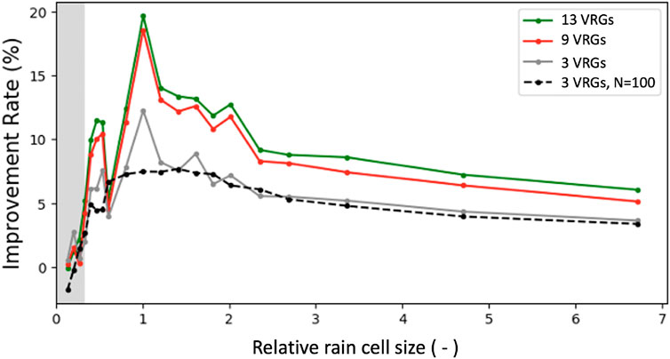
FIGURE 1. From Eshel et al. (2020)—RMSE improvement rate of cases where GMZ was applied in simulations where 3, 9, and 13 VRGs were assigned per CML, relative to the RMSE of the case of a single VRG per CML without GMZ. Results are plotted against the rainfall cell size normalized by the average length of CMLs in the network. A simulation with a larger dataset, solely for the case where GMZ was applied with three VRGs per CML, is displayed as well (dashed). GMZ constantly improves RMSE performance but has negligible additional contribution when more than nine VRGs are used. The grey shading marks the area where the reconstruction and the ground truth had a correlation coefficient
The foregoing implies that for a given area, both the specific subarea of interest (hinting at the density of the network) and the season (hinting at the rainfall’s spatial structure), which are local and temporal factors, respectively, should be considered, along with the desired preciseness. That said, note that the 20% improvement demonstrated here is confined to the single interpolation method tested in this study, IDW. Other more sophisticated methods may yield higher improvement rates.
A similar approach was used on real rainfall patterns, obtained from a radar product of the German Weather Service, for different aggregation intervals (Eshel et al., 2021), where the attenuation of an actual 808-CML network was simulated (referred to as a “semi-real” study). Here, the differences between the two cases were noticeable, but they were less significant than for the simplified Gaussian-shaped rain cells. In Eshel et al. (2021), however, the Kriging technique (spatial covariance-based interpolation) was also applied, showing similar results. A potential point of failure in GMZ as implemented in Eshel et al. (2021) was suggested for specific scenarios, where the redistribution of rain intensities between the VRGs on a given CML is more detrimental than assuming a single point in the center. The likeliness of such scenarios is conjectured to be very low when a single symmetric rain cell is in question, and to increase slightly the more spatially diverse the rain field is. This may explain differences between the results of Eshel et al. (2020) and Eshel et al. (2021). Nevertheless, on average, applying GMZ contributes to increasing accuracy, also in semi-real experiments.
In Zheng et al. (2022), the study of Eshel et al. (2020) was extended to the case where the spatial interpolation employs both CMLs and RGs. Here, the study is based on an actual CML network (see Figure 2A) where a CML is sometimes replaced by an RG located in its center. In each experiment, a growing number of CMLs were taken out of the network and replaced by a point measurement, that is, an RG based on their location. It is important to notice the difference between a VRG and an RG: The first refers to a location along a CML path (usually its center), which was chosen to represent a path-integrated measurement, whereas the latter is a point sampler of the rain field at its very location. In Zheng et al. (2022), nonisotropic GRCs (1) characterized by 6 parameters are assumed. The parameters defining the GRC, including the size and the orientation of the rain cell, have been chosen randomly and then “sampled” by the network according to (2), along with the addition of noise and quantization to simulate actual measurements. The IDW interpolation method was then used for rain field reconstruction, with GMZ as a preprocessing step in some scenarios. The resulting maps were later compared with the ground truth, to assess their performance. In Zheng et al. (2022), multiple points along the link represented the CML measurements and GMZ was utilized prior to the interpolation, where 11 VRGs were equally spaced along each CML path. In scenarios in which CMLs were replaced by RGs, the location of RGs was set randomly along the paths of discarded CMLs. The number of CMLs and RGs defines the scenario: Scenario S1 consists of CMLs only, while S5 consists of only RGs. In between, the number steadily decreases, such that S2, S3, and S4 consist of 7, 5, and 3 CMLs, respectively. For each of the 100 randomly generated GRCs, the replacement of randomly picked CMLs with RGs (done for S2-S4) was repeated 30 times. The decision about the random position of RG was made 100 times. It emerges from the above that S2-S4 consist of 300,000 experiments, S5 of 10,000 experiments, and S1 of only 100 experiments, since there was no need for random discard allocation. The map’s resolution is 5 m × 5 m. GRCs were created following (1), where ρ was randomly chosen between 0 and 1; locations of (μx, μy) were randomly assigned; and values of R0 were randomly selected from 10 to 50 mm/h, and the minimum rainfall intensity was set to 0.1 mmh−1. Following Marra and Morin (2018), σx was randomly chosen from 0.25 to 1.5 times the minimum side length of the study area; σy is randomly selected from 0.4 to 1 times σx. All random selections assume uniform distribution.
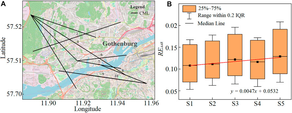
FIGURE 2. (A) Map of commercial microwave links in Zheng et al. (2022); (B) distribution of the relative error for average areal rainfall with 100 different simulated rain fields, for various types of near-ground sensor networks in the same location: from CMLs only (S1) to RGs only (S5). Each CML was represented by multiple VRGs determined by GMZ preprocessing. A growing number of CMLs were replaced by RGs in groups S1-S5, such that the number of CMLs was 10, 7, 5, 3, and 0, respectively, which represents a linear model. The positive slope indicates that the more CMLs are sampling the rain field, at the expense of RG, the smaller the error is.
As a performance evaluation metric, the normalized relative error of average areal rainfall (REAAR) was used:
where NT is the total number of pixels in the domain, and oi, ei are observations and estimates of ith pixel, respectively. The observations here are the simulated rain field (the ground truth) at each pixel, and the estimates are the reconstruction results, which are derived from the measurements of the simulated rain field by the assumed sensors, resulting the measurement vector y.
Figure 2B summarizes the distribution of the skill (Eq. 4) for the five different scenarios, indicating the median value of the REAAR. A clear trend can be noticed; the larger the CML/RG ratio is, the better the performance is. A linear model was fitted to median values of the boxplot distributions; thus, the slope serves as an indicator of the rate of the effect examined. The positive slope value implies that there is a loss in accuracy, on average, stemming from using a point and not a path measurement, since the median REAAR increases as more CMLs are discarded.
From these simulations, it emerges that, on average, the combined effect of applying GMZ and using a path integration measurement type yields higher accuracy in mapping. However, the performance improvement does not seem to be dramatic for the case of a small area with a relatively dense sensor network.
The best way to study the optimal potential performance of a parameter estimation problem, independently of the algorithm used, is by evaluating the Cramér–Rao bound (CRB) on the mean square estimation error. Formally, let
where the inequality A ≻ B for matrices A and B means that A− B ≻ 0,
The FIM can be evaluated for any given model that relates the parameter vector to the measurements, assuming that the probability density function (PDF) of measurements is known. For rain retrieval, the measurement vector y contains attenuation measurements from CMLs and rain measurements from RGs; the parameter vector θ fully characterizes the rain field. Assuming that the sensor measurements are independent, the FIM is given by:
where ξi is the ith sensor placement vector (e.g., position, length, and orientation),
When trying to apply the CRB to the problem of 2D rain retrieval from near-ground measurements by multiple sensors, a few difficulties arise:
(a) In general, rain fields are not described by parametric models.
(b) In cases where a parametric model is assumed to describe a rain cell, as in Messer et al. (2006), the estimation errors for the individual parameters are of limited interest.
(c) The statistical characteristics of the measurements by either CMLs or RGs are complex (Ostrometzky and Messer, 2020) because of quantization, nonlinear preprocessing, etc., thereby making the evaluation of the FIM challenging.
In Gat and Messer (2019), an elegant solution to (b) was proposed, using any assumed parametric model
where
where xi is the ith grid point along the x-axis, and yj is the jth grid point along the y-axis.
Regarding the other two difficulties (a) and (c), in Gat and Messer (2019), a simplified single symmetric GRC is characterized by four unknown parameters as in Eq. 1 with ρ = 0 and σx = σy = σ and additive white Gaussian noise is assumed. This simplified model was used to study the bound on the spatial MSErm 9) when either CMLs or RGs in the same locations are used for retrieving the 2D rain map. The sensors were located with a small perturbation around a uniform grid, and the length and orientation of CMLs were randomly set with exponential and uniform distributions, respectively.
Figure 3B depicts an example of the sensors used and the assumed rain cell. Figure 3A shows the resulting CRB on MSErm Eq. 9 for the case where all sensors are CMLs (solid line) or RGs (dashed line), as a function of the size of the rain cell for the case where the average length of CMLs is 3.5 km and the grid size is 2.5 km. It shows that when the size of the rain cell is small (relative to the grid size), CMLs outperform the mapping done by RGs. At a certain cell size, at the order of the average length of links, the performance crosses and the RGs’ mapping prevail slightly and asymptotically; when the cell size increases, the two sensors provide the same performance. In Gat and Messer (2019), it has shown that this crossing phenomenon always happens at a point that depends on the grid size and the average length of links.
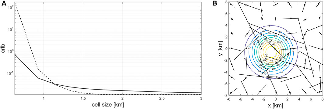
FIGURE 3. From Gat and Messer (2019)—(B) an example of the assumed rain cell and network of ground-level sensors. (A) The Cramér–Rao lower bound (noted in this figure as crlb) on the spatial mean square error (MSE) over the entire rain map for different sizes of the rain cells. Solid line—all sensors are line sensors (CMLs)—for example, the lines on (B); dashed lines—all sensors are point sensors (RGs)—for example, the points on (B).
One conjecture based on the analysis in Gat and Messer (2019), which is in agreement with the results of the analysis in Eshel et al. (2020), is that the use of CMLs in spotty rain fields may result in a significant performance advantage. In the sequel, we extend these results and show theoretically that this phenomenon occurs in a more realistic setting, where actual CML properties from the city of Gothenburg, Sweden, are used (Andersson et al., 2017). We compare three networks of sensors, where in all cases, the center of sensors is in the same locations (see Figure 4): a. All sensors are CMLs; b. all sensors are RGs; and c. a mixture of 60% CMLs and 40% RGs.
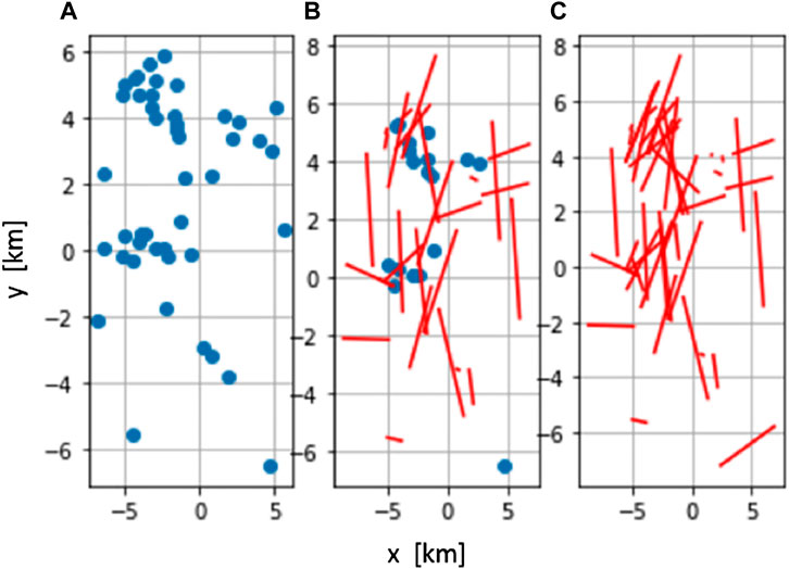
FIGURE 4. CML network in Gothenburg (Andersson et al., 2017)—(C); two simulated networks where all CMLs are replaced by RGs (A) or 40% of CMLs are randomly replaced by RGs (B).
In Figure 5, we present the CRB on the spatial MSE Eq. 9 derived similar to the result of Figure 3. Here as well, there is a clear advantage when a network of CMLs is used for retrieving small rain cells, but it is interesting to note that the performance of the mixed network is between that of CMLs and RGs only.
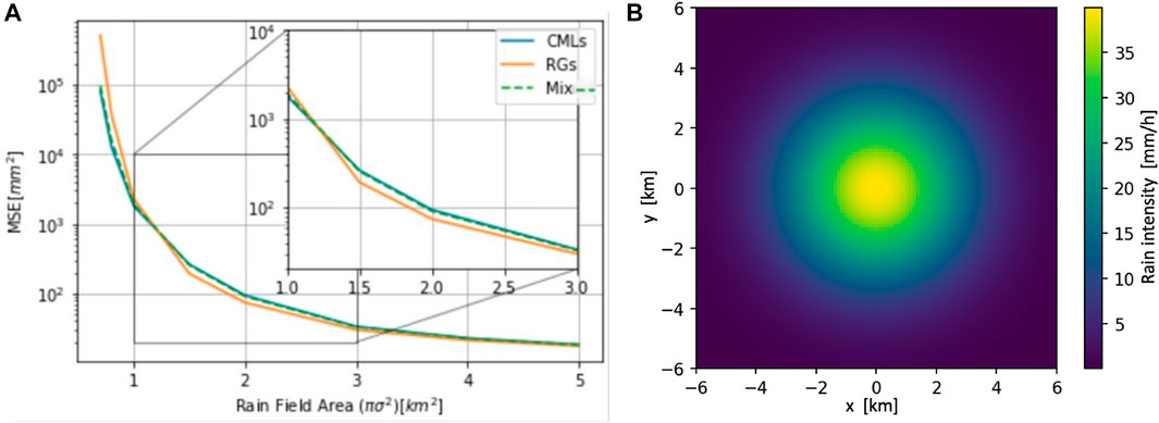
FIGURE 5. As in Figure 3 for the three sensor networks of Figure 4, where the GRC is located at (0, 0) with a peak rain intensity of 20 [mmh−1].
Figure 6 extends the results of Figure 5 for the case where the rain map is more complex. Here, three rain cells exist simultaneously (Figure 6A). The CRB on the spatial MSE depicted on the right shows similar features as in the case of a single rain cell. Moreover, both figures show high MSE in a small rain field. This is a result of a very low signal-to-noise ratio for most of the sensors due to a low rain intensity.
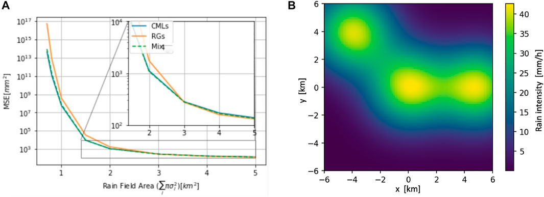
FIGURE 6. CRB on the spatial MSE as in Figure 5 (A) for multiple rain cells, as in (B). (A) presents the spatial MSE over the rain field area, which is the sum of cell sizes, and (B) presents the assumed rain field with three cells.
To overcome the first difficulty (a)—that actual rain fields do not obey parametric models—we present a CRB analysis of rain field mapping based on nonparametric B-spline representation of rain fields. In a nonparametric model, the rain is not modeled with a specific function, for example, a Gaussian-shaped function, but with different rain intensity levels for different locations in a noncorrelated manner. In this type of model, the estimated parameters are not intrinsic parameters of the rain model, such as rain cell size or rain cell center, but the actual rain intensities. In Sagiv and Messer (2022), the rain was modeled with B-spline functions, which have this property along with critical smoothness properties. B-splines are piecewise polynomial functions that are defined by two parameters: their order and the knots, the set of intervals on which each polynomial function is defined. They are generated in a recursive manner according to the Cox–De Boor formula (De Boor, 1972). B-splines are basis functions for spline functions; that is, any spline function of a given order and knots can be expressed as a linear combination of B-splines of that order and knots. Modeling the rain field as a 2D spline function, instead of Eq. 1, it can be described by a tensor product of B-spline functions (Sagiv and Messer, 2022):
where N(i,k)(t) represents the ith (corresponding to the ith knot) B-spline of order k, and Bij denote the ith and jth element of coefficient matrix
In Eq. 10, k and l correspond to the B-spline order on each axis, and θ = [B11, … , B1p, … , Bqp] corresponds to the B-spline coefficient matrix of the rain field. The results shown in the study considered B coefficients to be generated uniformly in [0, 1]. The selected distribution of coefficients was arbitrary, as the comparison tool chosen in the article is not dependent on them. For algorithmic purposes, more empirical research should be conducted to define the coefficient distribution in real-world rain cells.
This nonparametric model represents a wider range of rain field options. In particular, B-splines provide several properties that benefit the nonparametric modeling (De Boor, 1972). The first is spatial locality so that different areas in space are modeled using different parameters, reducing correlation between very distant points. The second is the smoothness of rain field, which can be controlled by adjusting the order of the B-splines. Smoothness is a key property of rain fields and is crucial for their representation. Figure 7 depicts an example of a simulated rain field, which was generated with 3rd-order B-spline functions.
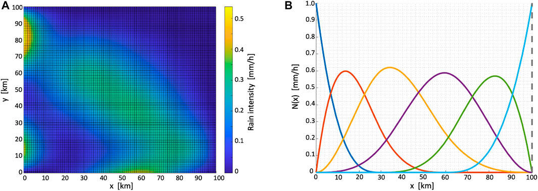
FIGURE 7. Example of a rain field created by 3rd-order B-splines (A) and demonstration of one-dimensional B-spline set (order = 3, knots = [0,10, 30, 60,100]) (B).
In Sagiv and Messer (2022), the performance of the estimation of the B-spline coefficients P using each type of sensors (CMLs as line projection sensors and RGs as point projection sensors) was examined through the Cramér–Rao lower bound, which was derived by calculating the projection matrix of each sensor on the set of the B-spline functions. Then, the CRB was averaged numerically over ms different sensor placements, resulting in the mean Cramér–Rao lower bound:
where Ψ is the distribution of the sensor spatial characteristics, and
Averaging the CRB over the different realization of sensor’s locations, angles, and lengths results in a performance bound that is not limited to a specific realization of sensor placements ψ. Instead, this result is influenced by sensor placement distribution Ψ, which generalized the results shown in Figures 3, 5, and 6 to a wider variety of sensor networks.
Figure 8 presents the mean CRB 11) of CMLs and RGs, where the rain field is represented by B-splines. It shows that CMLs outperform RGs when there is a low number of sensors, while the performance of both types of sensors becomes relatively similar when there is a large number of sensors. This phenomenon is explained by the high spatial coverage of CMLs. In contrast, rain gauges provide highly localized coverage. This means that the likelihood of a rain gauge sampling a B-spline in one of its tails is considerably higher than that of a CML, leading to less information retrieved by the sensor and a poorer signal-to-noise ratio. Therefore, CML-based estimation is better when there is a low number of measurements. For a large number of sensors, the spatial coverage is good using both types of sensors, leading to similar estimation performance. This result comes to show the importance of CMLs when designing a strong network with a limited number of sensors.
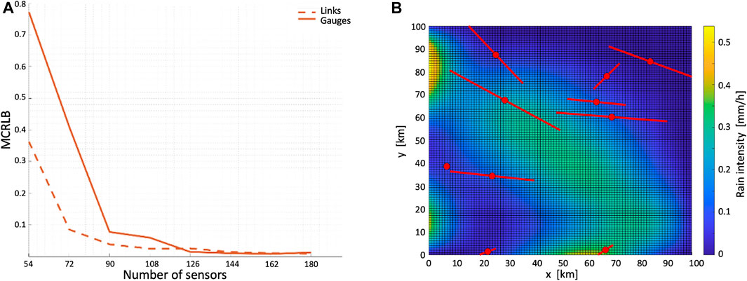
FIGURE 8. (A): Trace of the mean Cramér–Rao lower bound for 3rd-order B-spline with CMLs (dashed line) and RGs (solid line) as a function of the number of sensors in the given area (e.g., density). (B): An assumed network of CMLs and the corresponding RGs with a 2D map of the simulated rain field.
Generating a 2D rain field map from distributed near-ground sensors is a way to overcome the inherent limitations in remote sensing technologies. Until 2006, this task was impractical since the required number of sensors for sufficient accuracy was unrealistic if designated sensors were to be installed. The introduction of CMLs as opportunistic near-ground rain sensors (Messer et al., 2006) makes this task realistic. As shown in Gazit and Messer (2018b), the availability of CMLs in most areas on Earth is sufficient for reasonable accuracy of near-ground rain mapping. Indeed, despite technical challenges, appropriate tools were proposed, and operational software has been developed [e.g., Wolff et al. (2022)]. Since most proposed mapping techniques are based on spatial interpolation, originally proposed for point rain field sampling by rain gauges, the study of the relative performance of 2D rain field retrieval from CMLs is of great interest. In particular, a CML can be considered a noisy RG, and the good performance of CML-based rain mapping can be explained by their large quantity. However, CMLs sample a rain field different from an RG, and their line projection sampling operation can also introduce opportunities for improved mapping performance.
We present practical results where the performance of spatial interpolation-based rain mapping in various scenarios was compared. The results presented in Section 2 show that CMLs can indeed be considered virtual, noisy rain gauges, and in most cases, using them as such in spatial interpolation algorithms (together with existing RGs, if available) is empirically justified. However, if appropriate preprocessing of a CML’s measurement is applied to represent it with several VRGs along the link, even better mapping accuracy can be achieved, with the potential improvement being subject to the rain cell size–mean CML length relationship.
To isolate the algorithm dependency of the conclusions, Section 3 presents the Cramér–Rao analysis of the task of rain field retrieval, which provides a lower bound for the reconstruction accuracy. Here, hypothesized ideal RGs replace the noisy, virtual RGs used in the spatial interpolation algorithm, so the resulting bound is the lower bound for the performance of the common CML-based rain mapping algorithm. The results of the CRB analysis support the conclusions of Section 2, quantifying the performance gain of CMLs, depending on the characteristics of the rain field. In particular, it shows that the performance difference between CML and RG mapping becomes negligible when the rain field is smooth (relative to the topology of the sensor network).
From the foregoing, the following conclusions may be cautiously drawn: When the rain cell-to-CML length ratio is relatively small, the benefit of the larger spatial coverage of a CML (compared with that of a point measurement) exceeds the price paid in accuracy, stemming from the path integration of the sampled field. However, the relationships between the spatial coverage and the accuracy may turn over with the growth of this ratio, making a CML equivalent to not more than a noisy rain gauge. Then, in cases where this ratio is large enough, the differences become negligible.
The results presented in this study are for single-snapshot rain mapping. An interesting topic for future research would be to generalize them for the case where a time series of measurements from each sensor is available, such that the tempo-spatial rain field R (x, y; t), (x, y) ∈ AREA, t ∈ T is to be estimated, where AREA and T are the given area of interest and the time period, respectively.
Another direction for future research is the use of machine learning (instead of spatial interpolation) for 2D rain field mapping from measurements taken by CMLs or RGs. While the results of Section 3 are not influenced by the algorithm used, machine-learning algorithms, which have already demonstrated state-of-the-art results in transforming CMLs to VRG (Habi and Messer, 2020; Polz et al., 2020; Pudashine et al., 2020), may improve the performance of the interpolation algorithm. Moreover, the use of, for example, RGs for training and CMLs for mapping raises interesting questions about the role of various sensors in the task of near-ground rain field retrieval.
In addition, the theoretical results presented in this study contain gaps in the modeling of the measurements’ distribution. For example, the quantization effect in current measurements is ignored, but one could take this effect into account using the quantized CRB (Stoica et al., 2021). Moreover, higher order statistical effects are ignored by assuming a Gaussian noise model. A new approach called generative Cramér–Rao bound (Habi et al., 2022), which uses a data-driven approach to learn the measurements’ distribution, can be used to close these gaps.
HM is the leading author, was responsible for integrating the material, supervised the co-authors, and wrote the manuscript. AE and XZ contributed to Section 2. HH and SS contributed to Section 3. AE and HH edited the manuscript.
The authors declare that the research was conducted in the absence of any commercial or financial relationships that could be construed as a potential conflict of interest.
All claims expressed in this article are solely those of the authors and do not necessarily represent those of their affiliated organizations, or those of the publisher, the editors, and the reviewers. Any product that may be evaluated in this article, or claim that may be made by its manufacturer, is not guaranteed or endorsed by the publisher.
This work was done within the CellEnMon Lab at Tel Aviv University (https://cellenmonlab.tau.ac.il/), and the authors would like to express their sincere thanks to all past and present members of the research group. They also thank the various funding agencies that supported the work over the years, and the communication companies that share us their data. Special thanks to the group’s co-leaders Prof. Pinhas Alpert and Dr. Jonatan Ostrometzky.
Andersson, J., Berg, P., Hansryd, J., Jacobsson, A., Olsson, J., and Wallin, J. (2017). “Microwave links improve operational rainfall monitoring in gothenburg, Sweden,” in Proceeding of the 15th International Conference on Environmental Science and Technology, Rhodes, Greece, August–September 2017, 1–4. Available at: https://www.smhi.se/en/services/professional-services/memo-microwave-based-environmental-monitoring.
Berne, A., and Krajewski, W. F. (2013). Radar for hydrology: Unfulfilled promise or unrecognized potential? Adv. Water Resour. 51, 357–366. doi:10.1016/j.advwatres.2012.05.005
Chwala, C., and Kunstmann, H. (2019). Commercial microwave link networks for rainfall observation: Assessment of the current status and future challenges. WIREs Water 6, e1337. doi:10.1002/wat2.1337
Chwala, C., Leijnse, H., Overeem, A., Uijlenhoet, R., Messer, H., Alpert, P., et al. (2018). “Rainfall observation using commercial microwave links: An overview of ongoing projects around the globe,” in Proceeding of the 9th Workshop of the International Precipitation Working Group (IPWG).
COST-action (2021). Opportunistic precipitation sensing network. Available at: https://www.cost.eu/actions/ca20136/.
de Boor, C. (1972). On calculating with b-splines. J. Approx. theory 6, 50–62. doi:10.1016/0021-9045(72)90080-9
Eshel, A., Messer, H., Kunstmann, H., Alpert, P., and Chwala, C. (2021). Quantitative analysis of the performance of spatial interpolation methods for rainfall estimation using commercial microwave links. J. Hydrometeorol. 22, 831–843. doi:10.1175/jhm-d-20-0164.1
Eshel, A., Ostrometzky, J., Gat, S., Alpert, P., and Messer, H. (2020). Spatial reconstruction of rain fields from wireless telecommunication networks-scenario-dependent analysis of IDW-based algorithms. IEEE Geosci. Remote Sens. Lett. 17, 770–774. doi:10.1109/lgrs.2019.2935348
Gat, S., and Messer, H. (2019). “A comparative study of the performance of parameter estimation of a 2-d field using line-and point-projection sensors,” in Proceeding of the 2019 IEEE 8th International Workshop on Computational Advances in Multi-Sensor Adaptive Processing (CAMSAP), Le gosier, Guadeloupe, December 2019 (IEEE), 146–150. doi:10.1109/camsap45676.2019.9022443
Gazit, L., and Messer, H. (2018a). Advancements in the statistical study, modeling, and simulation of microwave-links in cellular backhaul networks. Environments 5, 75. doi:10.3390/environments5070075
Gazit, L., and Messer, H. (2018b). Sufficient conditions for reconstructing 2-d rainfall maps. IEEE Trans. Geosci. Remote Sens. 56, 6334–6343. doi:10.1109/tgrs.2018.2836998
Goldshtein, O., Messer, H., and Zinevich, A. (2009). Rain rate estimation using measurements from commercial telecommunications links. IEEE Trans. Signal Process. 57, 1616–1625. doi:10.1109/tsp.2009.2012554
Habi, H. V., Messer, H., and Bresler, Y. (2022). Learning to bound: A generative cram\’er-rao bound. arXiv preprint arXiv:2203.03695.
Habi, H. V., and Messer, H. (2021). Recurrent neural network for rain estimation using commercial microwave links. IEEE Trans. Geosci. Remote Sens. 59, 3672–3681. doi:10.1109/tgrs.2020.3010305
Harrison, D., Driscoll, S., and Kitchen, M. (2000). Improving precipitation estimates from weather radar using quality control and correction techniques. Meteorol. App. 7, 135–144. doi:10.1017/s1350482700001468
ITU-R.838 (2005). Specific attenuation model for rain for use in prediction methods. ITU-R 838-3, 1992-1999-2003-2005
Kunstmann, H., Chwala, C., Keis, F., Smiatek, G., Jayyousi, A., Shadeed, S., et al. (2017). “Precipitation monitoring and future precipitation assessment under climate change,” in WSTA 12th Gulf Water Conference 28-30 March, 2017 Kingdom of Bahrain Water in the GCC…Towards Integrated Strategies, 166.
Lehmann, E. L., and Casella, G. (2006). Theory of point estimation. Springer Science & Business Media.
Marra, F., and Morin, E. (2018). Autocorrelation structure of convective rainfall in semiarid-arid climate derived from high-resolution x-band radar estimates. Atmos. Res. 200, 126–138. doi:10.1016/j.atmosres.2017.09.020
Messer, H. (2018). Capitalizing on cellular technology-opportunities and challenges for near ground weather monitoring †. Environments 5, 73. doi:10.3390/environments5070073
Messer, H., Zinevich, A., and Alpert, P. (2006). Environmental monitoring by wireless communication networks. Science 312, 713. doi:10.1126/science.1120034
Ostrometzky, J., and Messer, H. (2020). “Statistical signal processing approach for rain estimation based on measurements from network management systems,” in Proceeding of the ICASSP 2020-2020 IEEE International Conference on Acoustics, Speech and Signal Processing (ICASSP), Barcelona, Spain, May 2020 (IEEE), 9026–9030. doi:10.1109/icassp40776.2020.9054652
Overeem, A., Leijnse, H., and Uijlenhoet, R. (2013). Country-wide rainfall maps from cellular communication networks. Proc. Natl. Acad. Sci. U.S.A. 110, 2741–2745. doi:10.1073/pnas.1217961110
Polz, J., Chwala, C., Graf, M., and Kunstmann, H. (2020). Rain event detection in commercial microwave link attenuation data using convolutional neural networks. Atmos. Meas. Tech. 13, 3835–3853. doi:10.5194/amt-13-3835-2020
Pudashine, J., Guyot, A., Petitjean, F., Pauwels, V. R., Uijlenhoet, R., Seed, A., et al. (2020). Deep learning for an improved prediction of rainfall retrievals from commercial microwave links. Water Resour. Res. 56, e2019WR026255. doi:10.1029/2019wr026255
Roy, V., Gishkori, S., and Leus, G. (2016). Dynamic rainfall monitoring using microwave links. EURASIP J. Adv. Signal Process. 2016, 77. doi:10.1186/s13634-016-0367-6
Sagiv, S., and Messer, H. (2022). A cramer-rao based study of 2-d non parametric b-splines rain field estimation. submitted
Stoica, P., Shang, X., and Cheng, Y. (2022). The cramér-rao bound for signal parameter estimation from quantized data [lecture notes]. IEEE Signal Process. Mag. 39, 118–125. doi:10.1109/msp.2021.3116532
Uijlenhoet, R., Overeem, A., and Leijnse, H. (2018). Opportunistic remote sensing of rainfall using microwave links from cellular communication networks. WIREs Water 5, e1289. doi:10.1002/wat2.1289
van de Beek, C., Leijnse, H., Torfs, P., and Uijlenhoet, R. (2012). Seasonal semi-variance of Dutch rainfall at hourly to daily scales. Adv. Water Resour. 45, 76–85. doi:10.1016/j.advwatres.2012.03.023
Wolff, W., Overeem, A., Leijnse, H., and Uijlenhoet, R. (2022). Rainfall retrieval algorithm for commercial microwave links: Stochastic calibration. Atmos. Meas. Tech. 15, 485–502. doi:10.5194/amt-15-485-2022
Keywords: rain estimation, Cramér–Rao bound, spatial interpolation, sensor network, commercial microwave links
Citation: Messer H, Eshel A, Habi HV, Sagiv S and Zheng X (2022) Rain Field Retrieval by Ground-Level Sensors of Various Types. Front. Sig. Proc. 2:877336. doi: 10.3389/frsip.2022.877336
Received: 16 February 2022; Accepted: 10 June 2022;
Published: 17 August 2022.
Edited by:
Juan Huo, Institute of Atmospheric Physics (CAS), ChinaReviewed by:
Venkat Roy, Rutgers, The State University of New Jersey, United StatesCopyright © 2022 Messer, Eshel, Habi, Sagiv and Zheng. This is an open-access article distributed under the terms of the Creative Commons Attribution License (CC BY). The use, distribution or reproduction in other forums is permitted, provided the original author(s) and the copyright owner(s) are credited and that the original publication in this journal is cited, in accordance with accepted academic practice. No use, distribution or reproduction is permitted which does not comply with these terms.
*Correspondence: H. Messer, bWVzc2VyQGVuZy50YXUuYWMuaWw=
Disclaimer: All claims expressed in this article are solely those of the authors and do not necessarily represent those of their affiliated organizations, or those of the publisher, the editors and the reviewers. Any product that may be evaluated in this article or claim that may be made by its manufacturer is not guaranteed or endorsed by the publisher.
Research integrity at Frontiers
Learn more about the work of our research integrity team to safeguard the quality of each article we publish.