Prediction of Treatment Response in Triple Negative Breast Cancer From Whole Slide Images

The automatic analysis of stained histological sections is becoming increasingly popular. Deep Learning is today the method of choice for the computational analysis of such data, and has shown spectacular results for large datasets for a large variety of cancer types and prediction tasks. On the other hand, many scientific questions relate to small, highly specific cohorts. Such cohorts pose serious challenges for Deep Learning, typically trained on large datasets. In this article, we propose a modification of the standard nested cross-validation procedure for hyperparameter tuning and model selection, dedicated to the analysis of small cohorts. We also propose a new architecture for the particularly challenging question of treatment prediction, and apply this workflow to the prediction of response to neoadjuvant chemotherapy for Triple Negative Breast Cancer.

1 Introduction

1.1 Context

Breast cancer (BC) is the most common cancer in women and the leading cause of cancer deaths with 18.2% of deaths among female cancer patients and 8% among all cancer patients (Institut National Du Cancer, 2019). Out of the four main breast cancer types, Triple Negative Breast Cancer (TNBC) represents 10% of all BC patients. This group has the worst prognostic with a five-year survival rate of around 77 percent versus 93 percent for the others. Currently no specialised treatments exists and the standard procedure consists in administrating neoadjuvant or adjuvant chemotherapy (Sakuma et al., 2011). TNBC research is still a very active field of study (Foulkes et al., 2010) and on the one hand, most works have focused on stratifying cohorts based on molecular and biological profiles (Lehmann et al., 2016). We, on the other hand, tackle the problem of predicting the response variable in a TNBC neoadjuvant chemotherapy (NACT) cohort from a histological needle-core biopsy section from the primary tumor prior to treatment. In contrast to most of the effort in cancer research, which is driven by the analysis of sequencing data, our study is based solely on the histological image data prior to treatment.

Each histological sample corresponds to tissue slides encompassing the tumor and its surrounding, stained with agents in order to highlight specific structures, such as cells, cell nuclei or collagen. The morphological properties of these elements and their spatial organisation have been linked to cancer subtypes, grades and prognosis. Even if pathologists have been trained to understand and report the evidence found in this type of data, the complexity, size and heterogeneity found in histological specimens make it highly unlikely that all relevant and exploitable patterns are known of today. Tissue images are informative about morphological and spatial patterns and are therefore inherently complementary to omics data.

Two major technological advances have triggered the emergence of the field of Computational Pathology: first, the arrival of new and powerful scanners replaced to some extent the use of conventional microscopes. Today, slides are scanned, stored and can be accessed rapidly at any moment (Huisman et al., 2010). This in turn has lead to the generation of large datasets that can also be analyzed computationally. The second element was the rise of new computer vision techniques.

Indeed, while the analysis of tissue slides has been of interest to the Computer Vision community for many years (Bartels et al., 1988), it is the advent of deep learning that has truly impacted the field. The advent of deep learning has stemmed a wide number of projects and investments. For visual systems, it is the combination of very large annotated dataset (Jia et al., 2009), hardware improvement and convolutional neural networks (CNN) that led to human-like capabilities. These outbreaks in performance have led to the creation of many annotated datasets and to the application of CNN’s to many tasks. However, for biomedical imaging in particular the application of CNN is not always straightforward:

1) The price for generating and annotating large biomedical dataset limits the progress of big data in this domain (Gurcan et al., 2009).

2) In histopathology in particular, each individual sample can be very large, one sample can be up to 60 GB uncompressed. This leads to multiple issues, again linked with the time and price needed for annotation, but also for the subsequent analysis where ad hoc methods have to be used as an entire image does not comfortably fit in RAM.

3) The nature of the data is inherently complex, each biological sample has its own individual patterns to be differentiated with relevant pathological evidence. For histopathology data, samples have a very large inter-slide, but also intra-slide variability that make the apparent signal harder to detect. In addition, the level of detail can be an additional difficulty: the relevant image features may be very fine grained, such as mitotic events, or very large such as the size of relevant image regions (necrotic, tumorous) (Janowczyk and Madabhushi, 2016).

In this paper, we set out to predict the response to NACT in TNBC from Whole Slide Images (WSI). Prediction of treatment response is one of the most difficult tasks in digital pathology (Echle et al., 2021). Unlike tasks like tumor detection and subtyping, for which high accuracies have been achieved in the past (Echle et al., 2021), there are no known morphological phenotypes that would allow for the prediction of treatment response. Moreover, datasets with treatment response are usually much smaller than datasets acquired in clinical routine for tasks such as automatic grading, metastasis detection or subtype prediction.

The contributions of this article are:

1) We benchmark several state-of-the-art architectures with respect to their performance in treatment response prediction.

2) We propose a new architecture for the prediction of treatment response and demonstrate its efficiency.

3) We propose a suitable model selection procedure that can cope with small datasets and avoids re-training, which is particularly important for deep learning. We prove its validity and efficiency on simulated data.

The paper is organised as follows: in the next Section 1.2 we describe related work. In Section 2, we describe the methodological developments. In Section 2.1, we present the limits of the current validation procedures and our alternative method used in this study. We then introduce our histopathology dataset in Section 2.3. Section 2.4 is devoted to introducing the DNN architectures which will be applied to the TNBC cohort. In Section 3, we show our results on the simulated data for our validation procedure and the application of our DNN to the TNBC cohort. Finally in Section 4 we discuss our methods and results.

1.2 Related Work

1.2.1 Challenges in Computational Pathology

The field of research in computational pathology can be divided in three categories:

1) Preprocessing, in particular color normalisation which aims at reducing the bias introduced by staining protocols used in different centers (Ruifrok and Johnston, 2001; Bejnordi et al., 2016).

2. Detection, segmentation and classification of objects of interest, such as regions (Bejnordi et al., 2017; Chan et al., 2019; Barmpoutis et al., 2021) and nuclei (Naylor et al., 2018; Graham et al., 2019).

3) The prediction of slide variables, such as presence and detection of disease (Litjens et al., 2018; Campanella et al., 2019), grading (Niazi et al., 2016; Ström et al., 2020), survival (Zhu et al., 2017; Courtiol et al., 2019), gene expression (Binder et al., 2018; Schmauch et al., 2020), genetic mutations (Coudray et al., 2018) or genetic signatures (Kather et al., 2020; Lazard et al., 2021).

Of note, these different of Computer Vision tasks have varying degrees of difficulty. For instance, Deep Learning based tumor detection and subtyping can be achieved with high accuracies [AUC: 0.97–0.99 for detection, AUC: 0.85–0.98 for subtyping, (Echle et al., 2021)]. This is not surprising, as these tasks rely on well-known visual cues. In contrast, prediction of treatment response is deemed one of the most difficult tasks in digital pathology (Echle et al., 2021), because the related morphological patterns are unknown and could potentially be very complex. It is even not clear to which extent treatment response is actually predictable from WSI.

Pipelines for slide variable predictions are usually divided into several steps. Tiles are partitioned into smaller images, usually referred to as patches or tiles, which are then encoded by a DNN, often trained on ImageNet (Zhu et al., 2017; Courtiol et al., 2019), as depicted in Figure 2. The training on ImageNet might be surprising at first sight, as the nature of the images are very different. In addition, ImageNet samples usually have a natural orientation, where the main object of interest is usually centered and scaled to fit in the image (Raghu et al., 2019). In contrast, histopathology images have a rotationally invariant content with no prior regarding scale or positioning of the relevant structures. However, rotational invariance can be imposed (Naylor et al., 2019; Lafarge et al., 2020), and in practice ImageNet based encodings are widely used and tend to perform very well.

After encoding of all tiles, each WSI is converted into a P × n_i matrix where P is the encoding size and n_i the number of tiles. The last step consists in aggregating tile level encodings to perform unsupervised or supervised predictions at the slide level (Zhu et al., 2017; Courtiol et al., 2018; Campanella et al., 2019; Courtiol et al., 2019; Naylor et al., 2019).

Computational Pathology as a field has benefited from the generation of large annotated data sets, mostly with pixel-level annotations (Kumar et al., 2017; Litjens et al., 2018; Naylor et al., 2018), or cell-level annotations (Veta et al., 2015) for cell classification. The major resource for WSI with slide level annotations are the Cancer Genome Atlas (TCGA) and the Camelyon Challenge (Litjens et al., 2018). These public repositories are paralleled by many in-house datasets (thus not accessible to the public), some of which can be very large, namely in a screening context, e.g., (Campanella et al., 2019). In most cases however, the datasets tend to be very small and fall therefore in the small n large p category. This is due to the fact that often the most interesting studies focus on particular molecularly defined cancer subtypes for which only small cohorts exist. In addition, collecting the output variable might be very challenging and time-consuming, if the project is not formulated in the context of Computer Aided Diagnosis. This is particularly true for treatment response prediction.

1.2.2 Challenges in Applying DNN to Small Datasets

For all supervised learning method it is custom to use a two step procedure for estimating the performance. After dividing your dataset into three categories: train, validation and test. The first step consists in performing model selection with the training and validation set. The second step simply involves evaluating the chosen model on the test set in order to assess an unbiased estimator of the performance (Pereira et al., 2009). This is however only possible if the three categories are large enough. When the validation set is too small and the discrepancy in the data too high, one could very easily over-fit or under-fit on the dataset (Varoquaux, 2018). When the number of samples n is small, which is usually the case for biomedical data, alternative validation methods have to be found such as cross-validation (CV) and nested cross-validation (NCV). CV is mostly used for model selection or assessing performance. NCV is used when the model needs a tuning based on an external dataset, such as hyperparameter tunning for Support Vector Machines. Even if these methods have been debated (Krstajic et al., 2014; Varoquaux, 2018; Wainer and Cawley, 2018), they are widely accepted. These methods are explained in more details in Section 2.1.

1.2.3 Prediction of the Response to Neoadjuvant Chemotherapy in Triple Negative Breast Cancer

Neoadjuvant chemotherapy (NACT) responses varies among patients in TNBC and no clear biological signal has been shown. Survival in these cohorts have been correlated to the Residual Cancer Burden (RCB) variable (Symmans et al., 2007) which can be used as a proxy for response. RCB is a pathological variable based on measurements of how much the primary tumor has shrunk and of the size of metastasis in axillary lymph nodes. Finding biological evidence to NACT response would allow for adequate and specific treatment, some histological variables have been found to be correlated with survival, such as the number Ki-67 positive cells (Elnemr et al., 2016), tumor infiltrating lymphocytes (Mao et al., 2016) and the Elston and Ellis grade (Elston and Ellis, 1991). Depending on the context, some alternative treatments have been found to help overall survival, such as those based on anthracycline and taxanes (Sakuma et al., 2011), carboplatin (Pandy et al., 2019) or with olaparib and talazoparib (Won and Spruck, 2020). Some treatments have emerged with targeted immunotherapy in combination with atezolizumab (anti-PD-L1 antibody) and nanoparticle albumin-bound (nab)-paclitaxel (Won and Spruck, 2020). Most of the studies for NACT responses have been performed in clinical practices and based on pathological variables (Elnemr et al., 2016; Gass et al., 2018; Zhu et al., 2020). In addition, some studies have analysed sequencing and molecular profiles in order to better understand and stratify cohorts (Lehmann et al., 2016; García-Vazquez et al., 2017; Wang et al., 2019).

To the best of our knowledge, it remains unclear whether and to which extent NACT response can be predicted from biopsies taken prior to treatment, and only few works have addressed this question so far (Naylor et al., 2019; Ogier du Terrail et al., 2021).

2 Materials and Methods

2.1 Validation Procedure

Here, we present our procedures to replace NCV in order to train DNN in a context of small n large p. We first explain cross-validation (CV), nested cross-validation (NCV) and their limitations. We propose two different procedures, better suited and show their effectiveness on a small case study.

2.1.1 Cross-Validation

CV is a common procedure for model evaluation or model selection, specifically in situations where the data set is relatively small. CV divides the initial data set into k_f folds, denoted ${\mathcal{F}}_1^{cv},{\mathcal{F}}_2^{cv},\dots ,{\mathcal{F}}_{k_f}^{cv}$ and runs algorithms on the data sets with one fold left out. We define, for all j, the set ${\mathcal{F}}_{-j}^{cv}$, which is the union of all folds expect for fold j:

${\mathcal{F}}_{-j}^{cv}=\bigcup _{\begin{array}{c}k\in [[1,k_f]]\\ k\ne j\end{array}}{\mathcal{F}}_k^{cv}$

2.1.1.1 Cross-Validation for Model Selection

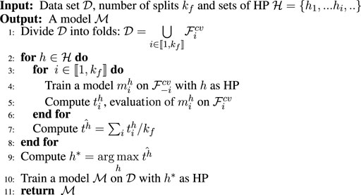
CV can be used for model selection or model tuning. The procedure that returns a tuned model $\mathcal{M}$ will be notated f^cv.

$\mathcal{M}=f^{cv}\left(\mathcal{D}\right)(1)$

We give the pseudo code in Algorithm 1, where $\mathcal{H}=h_1,\dots h_i,‥$ is the set of hyperparameters (HP).

Algorithm 1. Model selection, f^cv.

2.1.1.2 Cross-Validation for Model Evaluation

We can use CV to evaluate a given model and a HP set h. The procedure is similar to the pseudo code given in Algorithm 1, however we give in input a model and only one hyperparameter set and return $\widehat{t^h}$. In this case, $\widehat{t^h}$ is an unbiased estimator of the performance, as no optimization of the hyperparameters took place. If however several sets of hyperparameters are tested as to minimize the accuracy measured by cross-validation, this accuracy is an over-optimistic estimation of the true accuracy. In order to get a realistic estimation of the accuracy, we therefore have to turn to nested cross-validation.

2.1.1.3 Nested Cross-Validation

NCV is a procedure that allows one to tune a model and effectively report an unbiased estimation of the performance of the tuned model.

Given sets of HP and a data set $\mathcal{D}$, NCV corresponds to two nested loops of CV: The outer CV loop is for model evaluation, usually applied on test folds, sometimes referred to as outer folds. The inner CV loop is for model tuning, i.e., for each test fold, we perform a complete CV on the remaining data to correctly tune the model, and test the performance of the tuned model on data that has neither been used for training nor for HP tuning. We show the pseudo-code for NCV in Algorithm 2.

Algorithm 2. Nested cross-validation.

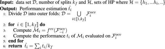
Another possible view is to see NCV as a simple CV for a model selection algorithm. For NCV, the model selection algorithm would be f^cv.It is important to note that as we are training DNN, we do not use a fixed hyperparameter set, $\mathcal{H}$, but randomly generate the set as it has been shown that randomised search performs better (Bergstra and Bengio, 2012).

2.1.2 Limitations

DNN training suffers from inherent randomness, as the loss function is highly non-convex and possess many symmetries (Bishop, 2006). In addition, there are some stochastic differences between training runs, such as the random initialization of the weight parameters and the data shuffling, naturally leading to different solutions. Especially for small datasets, these stochastic variations lead to notable differences in performance when we repeat training with the same hyperparameters.

In the classical setting, CV provides us with a set of hyperparameters that lead to a model with optimal performance, as estimated in the inner loop. For DNN trained on small datasets, there is no guarantee that the same set of hyperparameters will lead to similar performance, and for this reason retraining is not guaranteed to lead to a very good solution.

Another problem with the retraining in line 10 in Algorithm 1 is the use of early stopping. Early stopping is a very powerful regularization procedures that choses experimentally the point between the under- and over-fitting regime, but for this it requires a validation set. Early stopping would therefore not be applicable in the traditional CV-scheme with retraining.

2.1.3 Nested Ensemble Cross-Validation

Due to the incompatibility between NCV and early stopping we propose to modify the model selection procedure, i.e., function f^cv shown in Algorithm 1. In particular we do not perform retraining and return an ensemble of the models used during CV. Similarly to NCV, we perform a CV where we propose to modify f^cv into a better suited procedure, named f^ecv (ensemble cross-validation), shown in Algorithm 3.

Algorithm 3. Model selection, f^ecv.

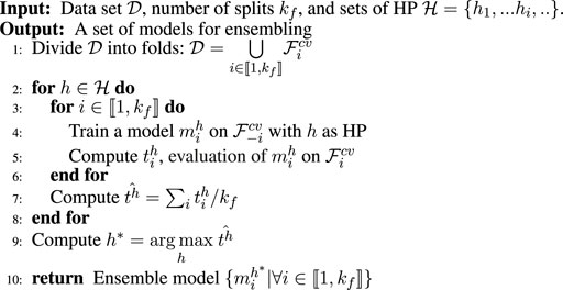
The main difference between f^cv and f^ecv is that we remove the final model retraining, i.e., line 10 of Algorithm 1 and give back the full set of k_f models trained for all folds for the maximizing hyperparameters; the prediction is obtained by ensembling these models.The advantage of this procedure is that we omit the retraining step which allows us to use early stopping for all individual models. In addition, we add another level of regularization by the ensembling. Of note, f^ecv can be used in an inner loop, too. This then leads to Nested Ensemble cross-validation (NECV).

2.1.4 Nested Best Fold Ensemble Cross-Validation

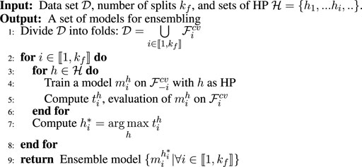
Similarly to the procedure NECV, we can define another procedure that we name NBFCV. NBFCV is based on f^bfcv defined in Algorithm 4. Compared to the preceding procedure, we inverted the two for-loops and retain the best model per fold. It then returns the ensemble of these selected models.

Algorithm 4. Model selection, f^bfcv.

2.2 Simulations

In order to compare and validate our procedure presented in Section 2.1 we propose to conduct a series of simulation studies where the results will be given in Section 3.1. In particular, we wish to demonstrate that DNN training given a set of HP can lead to inconsistent models and that NCV therefore might provide under-performing models compared to NECV and NBFCV, the proposed validation procedures.

2.2.1 Data Set Simulation

We simulated a simple balanced binary data, of size N = 350 in a medium to high dimensional setting with p = 256. We have ∀i ∈ [(1, N)], Y_i ∈ (−1, 1) and $X_i\sim \mathcal{N}(p_{y_i},\sigma I_p)$ where p_j is a cluster center, σ a given standard deviation and I_p the identity matrix of size p. We set one cluster center at p₁ = (1, 1, …, 1) and the second cluster center at p₋₁ = (−1, −1, … , −1). In Figures 1A–D respectively, we show four plots of the simulated data reduced to two dimensions thanks to a UMAP (McInnes et al., 2018), with standard deviations set to 2, 6, 10 and 14 respectively. Naturally, when the standard deviation increases the data becomes less separable.

FIGURE 1

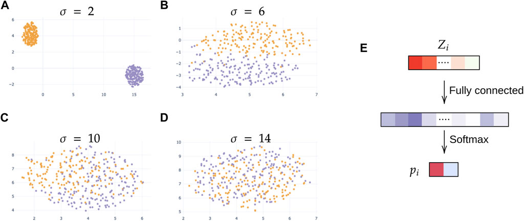
FIGURE 1. Data set simulation with p = 256 and model, (A) σ = 2, (B) σ = 6, (C) σ = 10, (D) σ = 14. (E) Simple two layer DNN model for predicting the class label.

2.2.2 Model

We apply a simple DNN model, composed of two layers, a first hidden layer with 256 hidden nodes and a classification layer with two nodes, the model is depicted in Figure 1E.

In particular, we minimise a cross-entropy error with an Adam optimiser and a batch size of 16. The tunable parameters are the weight-decay, drop out and learning rate. As an extra regularisation we use batch normalisation.

2.3 Application to Histopathology Data

2.3.1 Data Generation and Annotation

The data set used was generated at the Curie Institute and consists of annotated H&E stained histology needle core biopsy sections at 40× magnification sampled from a patient suffering from TNBC. In this paper, we evaluate the prediction of the response to treatment based solely on a biopsy sectioned prior to the treatment. As discussed in the introduction, not all patients respond to NACT, and we are therefore aiming at predicting the response to NACT based on the biopsy. In particular, each section was quality checked by expert histopathologists.

For each patient, we also collect WSI after surgery, allowing an expert pathologist to establish the residual cancer burden, as a proxy for treatment success. Out of the 336 samples that populate our data set, 167 were annotated as RCB-0, 27 as RCB-I, 113 as RCB-II and 29 as RCB-III. This data set is twice as large as the data set used in our previous study (Naylor et al., 2019). Similarly to this study, we refine the number of classes in order to avoid the problem of under-represented class. We investigate two prediction settings: 1) pCR (no residuum) vs. RCB (some residuum) and 2) pCR-RCB-I vs. RCB-II-III, which is clinically more relevant, as it is informative of a patient’s prognosis.

2.3.2 Data Encoding

As each biopsy section is relatively big, we wish to reduce the computational burden of feeding the entire biopsy to our algorithms. Instead, given a magnification factor, we divide each biopsy into tiles of equal sizes, 224 × 224 and project this tile into a lower dimensional space. We use a pre-trained DNN on ImageNet (Jia et al., 2009) such as ResNet (He et al., 2016) which produces a encoding of size 2048. This process is illustrated in Figure 2 where each biopsy section is converted into an encoded matrix of size n_i × P where P is the size of the resulting encoding and n_i the number of tiles tissue extracted from tissue i, $i\in \mathbb{N}$.

FIGURE 2

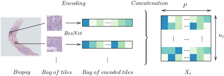
FIGURE 2. Encoding a biopsy.

In Table 1 we show the average number of tiles, $\overline{n_i}$ and variance at different magnification factors: highest resolution i.e. no down-sampling (2⁰ = 1), down-sampling by a factor 2¹ and by a factor 2² = 4.

TABLE 1

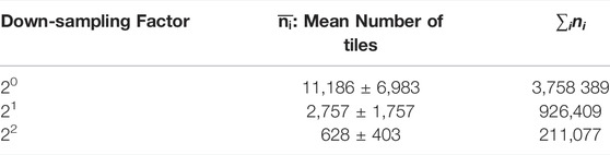
TABLE 1. Mean number of tiles.

The size of the data remains relatively large even after this reduction. We further reduce the size of the tile encoding with a PCA (Jolliffe, 2011), and project each tile encoding into a space approximately 10× smaller. By keeping 256 components, we keep 93.2% at 2⁰, 94.0% at 2¹ and 94.3% at a magnification factor of 2² of the explained variance.

2.3.3 Mathematical Framework

The data set will be denoted by $\mathcal{D}={(X_i,Y_i)}_{i\in [[1,N]]}$, where every item indexed by i in $\mathcal{D}$ is a joint variable (X_i, Y_i), N is the size of the data set, X_i is the input sample and Y_i the corresponding label. As described in the previous section, each tissue is represented by a bag of tiles of variable sizes, in particular ∀i ∈ [(1, N)], $X_i\in {\mathbb{R}}^{n_i\times P}$ and Y_i ∈ (0, 1) for task (1) or (2). This is simply a multiple instance learning framework, and such a framework has already been implemented for histopathological data (Xu et al., 2012, 2017; Courtiol et al., 2018; Couture et al., 2018). We simplify this framework by setting ∀i ∈ i ∈ [(1; N)], n_i = n_MF¹ which is set accordingly to the chosen magnification factor. For a given sample i, if n_i > n_MF we down-sample X_i, otherwise we up-sample X_i to the correct size. We evaluate our models by using the Area Under the Curve of the Receiver Operating Characteristic for measuring the performances in our two binary settings.

2.4 Neural Network Architectures

Today, DNN models for WSI classification usually consist in three steps: starting from encodings that are usually provided by pre-trained networks, a reduction layer might be applied, followed by an aggregation step that computes a slide level representation from the tile level representations and a final module that maps the slide level representation to the output variable.

In Figure 3, we show a basic example for such an architecture along these lines, with the three algorithmic blocks highlighted in gray. At the tile-level computation, we use 1D convolutions to transform the input encodings X_i into a more compact representation $X_i^{\prime }$. The tile representations $X_i^{\prime }$ are then summarized by a pooling layer, providing us with the biopsy section profile Z_i. For this, we can use a standard pooling layer such as an average pooling to quantify the abundance of specific tile patterns, or more complex, attention-based pooling, such as WELDON (Durand et al., 2016). Finally, from Z_i, the slide variable is predicted.

FIGURE 3

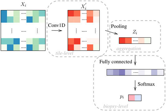
FIGURE 3. Model OneOne: tile encodings X_i from a pretrained network are projected to a more compact representations $X_i^{\prime }$ and then aggregated to build the slide representation Z_i, which is then used for prediction. Same colors indicate identical dimensions.

In this article, we test several encoding and agglomeration strategies which are explained in the next sections.

2.4.1 Encoding Projection

In Figure 3, the baseline architecture is illustrated (OneOne), with a 1D convolution for the tile level encoding and one fully connected layer at the slide level. In Figure 4, we test a deeper architecture for the encoding projections, consisting in three consecutive 1D convolutions, including bottleneck layers (depicted in orange), according to best practice in deep learning (Huang et al., 2017).

FIGURE 4

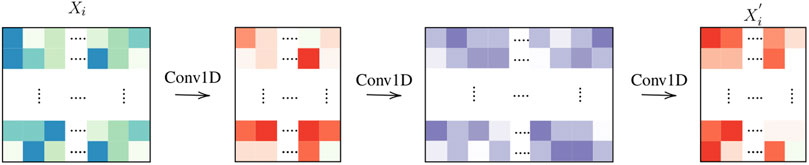
FIGURE 4. Tile computation: Three layers.

Furthermore, we also experiment with skip connections by concatenating the first tile representations to the final representation $X_i^{\prime }$ and by concatenating Z_i prior to the final softmax. We name this structure ThreeTwoSkip and illustrate it in Figure 5.

FIGURE 5

FIGURE 5. ThreeTwoSkip.

2.4.2 Pooling Layers

In terms of pooling layers, we experiment with: average pooling shown in Figure 6A, WELDON (Durand et al., 2016) shown in Figure 6B, a modified version of WELDON shown in Figure 6C and the concatenation of the first and the third is named WELDON-C (for context). The DNN that uses WELDON-C will be named CONAN².

FIGURE 6

FIGURE 6. Aggregation layers: (A) Average pooling; (B) WELDON pooling; (C) WELDON-C pooling which is WELDON concatenated with previous tile encoding.

The WELDON pooling is an attention-based layer which filters tiles based on a 1D convolution score. In particular, it retains the top and lowest $R\in {\mathbb{N}}^{*}$ achieving scores as Z_i. This architecture has shown excellent results for specific problems where the biological evidence lies in the detection of one type of specific tiles, like cancer regions (Courtiol et al., 2018). The method however suffers from identifiability issue, i.e., the model can not differentiate between two tiles achieving high or low score. In addition, the agglomeration strategy seems less promising in cases where the information resides in the percentage of tiles of a certain type. By providing a context in which a tile was selected, we allow the model to better differentiate between the selected tiles, thus allowing different tiles with different meanings to be selected, this can be particularly efficient when relevant information is based on different tile patterns.

We recap all the tested models in Table 2.

TABLE 2

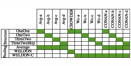
TABLE 2. Model architecture and pooling strategy, as described in the text. CHOWDER has been published previously (Courtiol et al., 2018).

2.4.3 Baseline Approach

In addition to comparing our proposed architectures to CHOWDER, we also compare them to a much simpler approach where we propagate the slide label to the tile level. If a slide is positive, then we assume all extracted tiles from this slide are positive, if a slide is negative, we assume that all tiles are negative. This is the simplest form of MIL. The training set is therefore huge, and we also known that there will be many errors, as many tiles do not contain any useful information regarding treatment response. Nevertheless, such an approach can work if there is a large fraction of informative tiles.

2.4.4 Model Tuning

We perform a random grid search for most parameters and only in suitable ranges. For the learning rate and weight decay we perform a random log sampling for a random scale associated to a random digit. We range from a scale of 10⁻⁶ to 10⁻³ for the learning rate and from 10⁻⁴ to 10⁻¹ for the weight decay. We randomly sample a drop out from a uniform ${\mathcal{U}}_{[0:0.4]}$. We randomly sample a bottleneck layer size from the following list (8, 32, 64) and the size of the larger representations are randomly sampled from (64, 128).

3 Results

3.1 Simulation Results

3.1.1 High Performance Variability in DNN Training

In Figure 7A, we show the average variance of our model with increasing standard deviation σ. In particular, for each σ, we generate 100 simulated dataset with a standard deviation of σ and train 1000 DNN on the same data and with the same HP. As this is simulated data, we evaluate the performance of each training on a large independently simulated test set instead of using the outer CV loop (Varoquaux, 2018). We found that setting the learning rate to 1.10⁻⁴, the weight decay to 5.10⁻³ and drop out to 0.4 tend to always return reasonable results for our simulation setting.

FIGURE 7

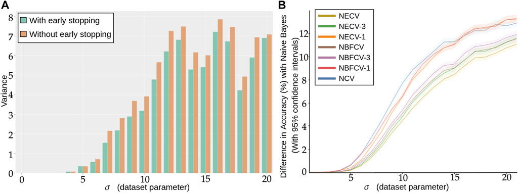
FIGURE 7. (A) Repeated training, with and without early stopping: (A) Performance Variance, as measured on an independently simulated test set, (B) Comparison of models trained with NCV, NECV and NBFCV. On the y-axis we have the difference in accuracy between the Naive Bayes model and a given validation approach. As the data distribution is known, the Naive Bayes is a theoretical upper limit of the achievable performance. Curves are shown with 95% confidence intervals. A lower curve implies a better score.

As the standard deviation σ of the simulated data increases, we expect more overlapping between our two classes and naturally, the classification accuracy decreases. For lower σ, regardless of using early stopping or not, the models reaches perfect scores.

In Figure 7, we observe that the more difficult the problem (larger σ), the lower the accuracy, but also the larger the variance: not only do we predict less well, but also does the performance variation increase, such that by retraining a model with the same hyperparameters is not guaranteed at all to provide a model with similar performance. We also see from Figure 7A that early stopping alleviates this problem and consistently reduces the variance in performance, in particular for higher σ.

3.1.2 Nested Cross-Validation Leads to Under-performing Models

We compare the performance of the proposed validation procedures to NCV with the number splits k_f = 5 in Figure 7B with 95% confidence intervals around the estimator. On the x-axis we have the standard deviation σ of the simulated data and on the y-axis we have the difference between the Naive Bayes estimator with the corresponding performance, therefore the lower the curve the better the procedure. In addition to Figure 7B, we give the corresponding accuracy score for each σ and validation procedure explicitly in Supplementary Table S1. As the dataset distribution is known, the Naive Bayes is the best classification rule that can be implemented and can be viewwed as an upper bound of the performance. For each σ, we collect 100 estimators with Algorithm 1, Algorithm 3 and Algorithm 4. Next, we compare several strategies for NECV and NBFCV: NECV-1/NBFCV-1, where we keep the best scoring model of the ensemble, NECV-3/NBFCV-3, where we keep the top 3 models and NECV/NBFCV, where we keep all five models.

We first notice that the NCV curve is lower or equal to any of the NECV/NBFCV curves. The best performing model is NECV—i.e., the average of all selected models from the inner CV. In particular NECV has a higher Accuracy than NCV by at least 2%. NBFCV under-performs by a slight margin compared to NECV and seems to be equivalent to NECV-3 in terms of performance.

We conclude that retraining the model without an outer validation score leads to lower overall performance and early stopping is a very useful regularization technique for small sample size problems.

3.2 Prediction of Response to Neoadjuvant Chemotherapy

We next applied the different architectures detailed in Section 2.4 (also summarized in Table 2) to the problem of the prediction of response to neoadjuvant chemotherapy in TNBC. We tested 3 different image resolutions (0, 1, 2), 0 being the highest resolution. In order to get realistic estimations of the performance, while using early stopping, we perform the validation proposed in Section 2.1. In Figures 8A,B we show the average AUC ROC performance on the residual and prognostic prediction tasks, for all methods shown in Table 2 and for all resolution levels.

FIGURE 8

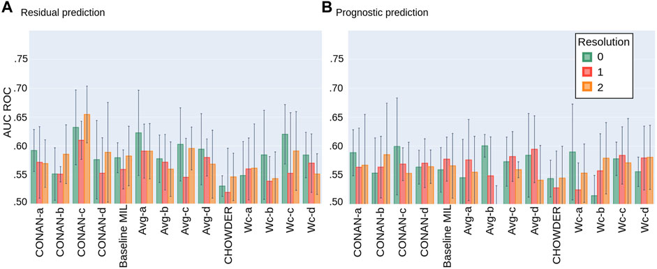
FIGURE 8. Average AUC ROC performance with standard deviation on five fold NECV on the task of predicting: (A) residual cancer and (B) patient prognostic in TNBC.

For the task of predicting the residual cancer, the best performing model would be the CONAN-c model at resolution 2 with an AUC of 0.654 ± 0.049. Others model’s performance range in between 0.55 and 0.60 of AUC with higher standard deviations. Models at resolution 0 seem to generally achieve higher scores then those at lower resolutions. Model architecture c seem to be better suited for this task than the others. The Average concatenated to WELDON-C pooling seems to perform slightly better then the rest. The method CHOWDER which gave excellent results on CAMELYON for cancer detection (Courtiol et al., 2018) and which has been a state-of-the-art solution in the field under-performs on our dataset for response prediction.

For the task of predicting the patient prognostic, the best performing model would be the Avg-b model at resolution 0 with an AUC of 0.601 ± 0.019. CONAN-c at resolution 2 performs similarly but with a much higher standard deviation. Neither resolution, nor model architecture and pooling layer seem to unanimously be better then the others. However, CHOWDER under-performs compared to the other proposed methods.

4 Discussion

In this study, we set out to predict the response to neoadjuvant chemotherapy in TNBC from biopsies taken before treatment. A system that would allow to predict this response with high accuracy could help identifying patients with no or little benefit of the treatment and therefore spare them the heavy burden of the therapy.

From a methodological point of view, this is particularly challenging for three reasons: first, we do not know to which extent the relevant information is actually present in the image data. In addition, even if the relevant information is contained in the slide, the complexity of the related patterns is unclear. Second, biopsies only capture a part of the relevant information, as they are only a localized sample of the tumor. Third, as this is a project regarding a specific subtype, the cohort is relatively small, unlike many pan-cancer cohorts used in large Computational Pathology projects (Campanella et al., 2019).

In order to solve this problem, we have developed the model CONAN, that combines the power of selecting K tiles (top and bottom), but keeps both the ranking scores and the full tile descriptions to build the slide representation. We have compared this model with a number of different architectures, and achieved an AUC of 0.65.

We also tackled an important problem of model selection with cross-validation, a crucial step in particular for small datasets. We found that the retraining step in classical Nested cross-validation can lead to lower performances for small N, because the training is highly variable, and a network retrained with the optimal set of hyperparameters is not guaranteed at all to be optimal itself. We therefore have proposed a new cross-validation procedure relying on ensembling rather than retraining, and thus allowing to use early stopping as a regularization method.

Nevertheless, we must conclude that the prediction of treatment response is probably one of the hardest problems in Computational Pathology, and that even though we see that there is some degree of predictability, the results still seem far from clinical applicability. Also, another problem that is not addressed in this study is the applicability of trained networks across different centers. Clearly, we need more data to tackle these challenging questions. But it is also likely that even with much more data, AUCs will not reach very high levels by looking at biopsies alone. A promising avenue would therefore be to use other kinds of data in addition to histopathology data.

Data Availability Statement

The datasets presented in this article are not readily available because they are the property of Institut Curie. Requests to access the datasets should be directed to thomas.walter@mines-paristech.fr.

Author Contributions

PN was main contributor, developed the methods and code and generated the results. TL helped with the code. FR and TW designed the project. GB, ML, AVC, A-SH, and FR generated the cohort. GB and ML provided interpretation of the biological results. TW supervised the project. PN and TW wrote the paper.

Funding

PN was funded by the Ligue Contre le Cancer. TL was supported by a Q-Life PhD fellowship (Q-life ANR-17-CONV-0005). Furthermore, this work was supported by the French government under man-agement of Agence Nationale de la Recherche as part of the “Investissements d’avenir” program, reference ANR-19-P3IA-0001 (PRAIRIE 3IA Institute).

Conflict of Interest

The authors declare that the research was conducted in the absence of any commercial or financial relationships that could be construed as a potential conflict of interest.

Publisher’s Note

All claims expressed in this article are solely those of the authors and do not necessarily represent those of their affiliated organizations, or those of the publisher, the editors and the reviewers. Any product that may be evaluated in this article, or claim that may be made by its manufacturer, is not guaranteed or endorsed by the publisher.

Acknowledgments

The authors would like to thank André Nicolas from the PathEx platform, Service the Pathologie, Institut Curie, Paris, where the images have been acquired.

Supplementary Material

The Supplementary Material for this article can be found online at: https://www.frontiersin.org/articles/10.3389/frsip.2022.851809/full#supplementary-material

Footnotes

¹For Magnification Factor.

²Context cOncatenated tile selection NeurAl Network

References

Barmpoutis, P., Di Capite, M., Kayhanian, H., Waddingham, W., Alexander, D. C., Jansen, M., et al. (2021). Tertiary Lymphoid Structures (TLS) Identification and Density Assessment on H&E-stained Digital Slides of Lung Cancer. Plos one 16, e0256907. doi:10.1371/journal.pone.0256907

PubMed Abstract | CrossRef Full Text | Google Scholar

Bartels, P. H., Weber, J. E., and Duckstein, L. (1988). Machine Learning in Quantitative Histopathology. Anal. Quant Cytol. Histol. 10, 299–306.

PubMed Abstract | Google Scholar

Bejnordi, B. E., Lin, J., Glass, B., Mullooly, M., Gierach, G. L., Sherman, M. E., et al. (2017). Deep Learning-Based Assessment of Tumor-Associated Stroma for Diagnosing Breast Cancer in Histopathology Images.” in 2017 IEEE 14th international symposium on biomedical imaging (ISBI 2017), 929. doi:10.1109/isbi.2017.7950668

CrossRef Full Text | Google Scholar

Bergstra, J., and Bengio, Y. (2012). Random Search for Hyper-Parameter Optimization. J. machine Learn. Res. 13, 281–305.

Google Scholar

Binder, A., Bockmayr, M., Hägele, M., Wienert, S., Heim, D., Hellweg, K., et al. (2018). Towards Computational Fluorescence Microscopy: Machine Learning-Based Integrated Prediction of Morphological and Molecular Tumor Profiles. arXiv preprint arXiv:1902.07208.

Google Scholar

Bishop, C. M. (2006). Pattern Recognition. Machine Learn., 225–290.

Google Scholar

Campanella, G., Hanna, M. G., Geneslaw, L., Miraflor, A., Werneck Krauss Silva, V., Busam, K. J., et al. (2019). Clinical-grade Computational Pathology Using Weakly Supervised Deep Learning on Whole Slide Images. Nat. Med. 25, 1301–1309. doi:10.1038/s41591-019-0508-1

PubMed Abstract | CrossRef Full Text | Google Scholar

Chan, L., Hosseini, M. S., Rowsell, C., Plataniotis, K. N., and Damaskinos, S. (2019). Histosegnet: Semantic Segmentation of Histological Tissue Type in Whole Slide Images.” in Proceedings of the IEEE/CVF International Conference on Computer Vision. 10662doi:10.1109/iccv.2019.01076

CrossRef Full Text | Google Scholar

Chollet, F. (2015). Keras. GitHub. Available at: https://github.com/fchollet/keras.

Google Scholar

Coudray, N., Ocampo, P. S., Sakellaropoulos, T., Narula, N., Snuderl, M., Fenyö, D., et al. (2018). Classification and Mutation Prediction from Non-small Cell Lung Cancer Histopathology Images Using Deep Learning. Nat. Med. 24, 1559–1567. doi:10.1038/s41591-018-0177-5

PubMed Abstract | CrossRef Full Text | Google Scholar

Courtiol, P., Maussion, C., Moarii, M., Pronier, E., Pilcer, S., Sefta, M., et al. (2019). Deep Learning-Based Classification of Mesothelioma Improves Prediction of Patient Outcome. Nat. Med. 25, 1519–1525. doi:10.1038/s41591-019-0583-3

PubMed Abstract | CrossRef Full Text | Google Scholar

Courtiol, P., Tramel, E. W., Sanselme, M., and Wainrib, G. (2018). Classification and Disease Localization in Histopathology Using Only Global Labels: A Weakly-Supervised Approach. arXiv preprint arXiv:1902.07208.

Google Scholar

Couture, H. D., Marron, J. S., Perou, C. M., Troester, M. A., and Niethammer, M. (2018). Multiple Instance Learning for Heterogeneous Images: Training a CNN for Histopathology. Lecture Notes Comp. Sci., 11071, 254–262. doi:10.1007/978-3-030-00934-2_29

CrossRef Full Text | Google Scholar

di Tommaso, P., Chatzou, M., Floden, E. W., Barja, P. P., Palumbo, E., and Notredame, C. (2017). Nextflow Enables Reproducible Computational Workflows. Nat. Biotechnol. 35, 316–319. doi:10.1038/nbt.3820

PubMed Abstract | CrossRef Full Text | Google Scholar

Durand, T., Thome, N., and Cord, M. (2016). “WELDON: Weakly Supervised Learning of Deep Convolutional Neural Networks,” in Proceedings of the IEEE Computer Society Conference on Computer Vision and Pattern Recognition, Las Vegas, Nevada, June 27–30, 4743–4752. doi:10.1109/CVPR.2016.513

CrossRef Full Text | Google Scholar

Echle, A., Rindtorff, N. T., Brinker, T. J., Luedde, T., Pearson, A. T., and Kather, J. N. (2021). Deep Learning in Cancer Pathology: a New Generation of Clinical Biomarkers. Br. J. Cancer 124, 686–696. doi:10.1038/s41416-020-01122-x

PubMed Abstract | CrossRef Full Text | Google Scholar

Ehteshami Bejnordi, B., Litjens, G., Timofeeva, N., Otte-Höller, I., Homeyer, A., Karssemeijer, N., et al. (2016). Stain Specific Standardization of Whole-Slide Histopathological Images. IEEE Trans. Med. Imaging 35, 404–415. doi:10.1109/TMI.2015.2476509

PubMed Abstract | CrossRef Full Text | Google Scholar

Elnemr, G. M., El-Rashidy, A. H., Osman, A. H., Issa, L. F., Abbas, O. A., Al-Zahrani, A. S., et al. (2016). Response of Triple Negative Breast Cancer to Neoadjuvant Chemotherapy: Correlation between Ki-67 Expression and Pathological Response. Asian Pac. J. Cancer Prev. 17, 807–813. doi:10.7314/apjcp.2016.17.2.807

PubMed Abstract | CrossRef Full Text | Google Scholar

Elston, C. W., and Ellis, I. O. (1991). Pathological Prognostic Factors in Breast Cancer. I. The Value of Histological Grade in Breast Cancer: Experience from a Large Study with Long-Term Follow-Up. Histopathology 19, 403–410. doi:10.1111/j.1365-2559.1991.tb00229.x

PubMed Abstract | CrossRef Full Text | Google Scholar

Foulkes, W. D., Smith, I. E., and Reis-Filho, J. S. (2010). Triple-negative Breast Cancer. N. Engl. J. Med. 363, 1938–1948. doi:10.1056/NEJMra1001389

PubMed Abstract | CrossRef Full Text | Google Scholar

García-Vazquez, R., Ruiz-García, E., Meneses García, A., Astudillo-De La Vega, H., Lara-Medina, F., Alvarado-Miranda, A., et al. (2017). A Microrna Signature Associated with Pathological Complete Response to Novel Neoadjuvant Therapy Regimen in Triple-Negative Breast Cancer. Tumour Biol. 39, 1010428317702899. doi:10.1177/1010428317702899

PubMed Abstract | CrossRef Full Text | Google Scholar

Gass, P., Lux, M. P., Rauh, C., Hein, A., Bani, M. R., Fiessler, C., et al. (2018). Prediction of Pathological Complete Response and Prognosis in Patients with Neoadjuvant Treatment for Triple-Negative Breast Cancer. BMC cancer 18, 1051–1058. doi:10.1186/s12885-018-4925-1

PubMed Abstract | CrossRef Full Text | Google Scholar

Graham, S., Vu, Q. D., Raza, S. E. A., Azam, A., Tsang, Y. W., Kwak, J. T., et al. (2019). Hover-Net: Simultaneous Segmentation and Classification of Nuclei in Multi-Tissue Histology Images 58. doi:10.1016/j.media.2019.101563

PubMed Abstract | CrossRef Full Text | Google Scholar

Gurcan, M. N., Boucheron, L. E., Can, A., Madabhushi, A., Rajpoot, N. M., and Yener, B. (2009). Histopathological Image Analysis: A Review. IEEE Rev. Biomed. Eng. 2, 147–171. doi:10.1109/rbme.2009.2034865

PubMed Abstract | CrossRef Full Text | Google Scholar

He, K., Zhang, X., Ren, S., and Sun, J. (2016). “Deep Residual Learning for Image Recognition,” in Proceedings of the IEEE conference on computer vision and pattern recognition, Las Vegas, Nevada, June 27–30, 770–778. doi:10.1109/CVPR.2016.90

CrossRef Full Text | Google Scholar

Huang, G., Liu, Z., Van Der Maaten, L., and Weinberger, K. Q. (2017). “Densely Connected Convolutional Networks,” in Proceedings - 30th IEEE Conference on Computer Vision and Pattern Recognition, Honolulu, Hawaii, July 22–25. (Los Alamitos, California: IEEE Computer Society, Conference Publishing Services), 2261–2269. Available at: https://www.worldcat.org/title/proceedings-30th-ieee-conference-on-computer-vision-and-pattern-recognition-21-26-july-2016-honolulu-hawaii/oclc/1016407672. doi:10.1109/CVPR.2017.243

CrossRef Full Text | Google Scholar

Huisman, A., Looijen, A., van den Brink, S. M., and van Diest, P. J. (2010). Creation of a Fully Digital Pathology Slide Archive by High-Volume Tissue Slide Scanning. Hum. Pathol. 41, 751–757. doi:10.1016/j.humpath.2009.08.026

PubMed Abstract | CrossRef Full Text | Google Scholar

InstitutNational Du Cancer (2019). Les chiffres du cancer du sein en France.

Google Scholar

Janowczyk, A., and Madabhushi, A. (2016). Deep Learning for Digital Pathology Image Analysis: A Comprehensive Tutorial with Selected Use Cases. J. Pathol. Inform. 7, 29. doi:10.4103/2153-3539.186902

PubMed Abstract | CrossRef Full Text | Google Scholar

Jia, D., Dong, W., Socher, R., Li, L., Li, K., and Fei-Fei, Li. (2009). ImageNet: A Large-Scale Hierarchical Image Database. CVPR, 248–255. doi:10.1109/cvprw.2009.5206848

CrossRef Full Text | Google Scholar

Jolliffe, I. (2011). Principal Component Analysis. Springer.

Google Scholar

Kather, J. N., Heij, L. R., Grabsch, H. I., Loeffler, C., Echle, A., Muti, H. S., et al. (2020). Pan-cancer Image-Based Detection of Clinically Actionable Genetic Alterations. Nat. Cancer 1, 789–799. doi:10.1038/s43018-020-0087-6

PubMed Abstract | CrossRef Full Text | Google Scholar

Krstajic, D., Buturovic, L. J., Leahy, D. E., and Thomas, S. (2014). Cross-validation Pitfalls when Selecting and Assessing Regression and Classification Models. J. Cheminform 6, 10–15. doi:10.1186/1758-2946-6-10

PubMed Abstract | CrossRef Full Text | Google Scholar

Kumar, N., Verma, R., Sharma, S., Bhargava, S., Vahadane, A., and Sethi, A. (2017). A Dataset and a Technique for Generalized Nuclear Segmentation for Computational Pathology. IEEE Trans. Med. Imaging 36, 1550–1560. doi:10.1109/TMI.2017.2677499

PubMed Abstract | CrossRef Full Text | Google Scholar

Lafarge, M. W., Bekkers, E. J., Pluim, J. P. W., Duits, R., and Veta, M. (2020). Roto-Translation Equivariant Convolutional Networks: Application to Histopathology Image Analysis. Med. Image Anal. 68, 101849. doi:10.1016/j.media.2020.101849

PubMed Abstract | CrossRef Full Text | Google Scholar

Lazard, T., Bataillon, G., Naylor, P., Popova, T., Bidard, F.-C., Stoppa-Lyonnet, D., et al. (2021). Deep Learning Identifies New Morphological Patterns of Homologous Recombination Deficiency in Luminal Breast Cancers from Whole Slide Images. Preprint, Cancer Biol. doi:10.1101/2021.09.10.459734

CrossRef Full Text | Google Scholar

Lehmann, B. D., Jovanović, B., Chen, X., Estrada, M. V., Johnson, K. N., Shyr, Y., et al. (2016). Refinement of Triple-Negative Breast Cancer Molecular Subtypes: Implications for Neoadjuvant Chemotherapy Selection. PloS one 11, e0157368. doi:10.1371/journal.pone.0157368

PubMed Abstract | CrossRef Full Text | Google Scholar

Litjens, G., Bandi, P., Ehteshami Bejnordi, B., Geessink, O., Balkenhol, M., Bult, P., et al. (2018). 1399 H&E-stained sentinel Lymph Node Sections of Breast Cancer Patients: the CAMELYON Dataset. GigaScience 7, 65. doi:10.1093/gigascience/giy065

PubMed Abstract | CrossRef Full Text | Google Scholar

Mao, Y., Qu, Q., Chen, X., Huang, O., Wu, J., and Shen, K. (2016). The Prognostic Value of Tumor-Infiltrating Lymphocytes in Breast Cancer: a Systematic Review and Meta-Analysis. PloS one 11, e0152500. doi:10.1371/journal.pone.0152500

PubMed Abstract | CrossRef Full Text | Google Scholar

McInnes, L., Healy, J., Saul, N., and Großberger, L. (2018). UMAP: Uniform Manifold Approximation and Projection. Joss 3, 861. doi:10.21105/joss.00861

CrossRef Full Text | Google Scholar

Naylor, P., Boyd, J., Laé, M., Reyal, F., and Walter, T. (2019). Predicting Residual Cancer burden in a Triple Negative Breast Cancer Cohort.” in Proceedings - International Symposium on Biomedical Imaging, doi:10.1109/ISBI.2019.8759205

CrossRef Full Text | Google Scholar

Naylor, P., Laé, M., Reyal, F., and Walter, T. (2019). Segmentation of Nuclei in Histopathology Images by Deep Regression of the Distance Map. IEEE Trans. Med. Imaging 38, 448–459. doi:10.1109/TMI.2018.2865709

PubMed Abstract | CrossRef Full Text | Google Scholar

Niazi, M. K. K., Keluo Yao, K., Zynger, D. L., Clinton, S. K., Chen, J., Koyutürk, M., et al. (2016). Visually Meaningful Histopathological Features for Automatic Grading of Prostate Cancer. IEEE J. Biomed. Health Inform. 21, 1027–1038. doi:10.1109/JBHI.2016.2565515

PubMed Abstract | CrossRef Full Text | Google Scholar

Ogier du Terrail, J., Leopold, A., Joly, C., Beguier, C., Andreux, M., Maussion, C., et al. (2021). Collaborative Federated Learning behind Hospitals’ Firewalls for Predicting Histological Response to Neoadjuvant Chemotherapy in Triple-Negative Breast Cancer. medRxiv. Available at: https://www.medrxiv.org/content/10.1101/2021.10.27.21264834v1.

Google Scholar

Pandy, J. G. P., Balolong-Garcia, J. C., Cruz-Ordinario, M. V. B., and Que, F. V. F. (2019). Triple Negative Breast Cancer and Platinum-Based Systemic Treatment: a Meta-Analysis and Systematic Review. BMC cancer 19, 1065–1069. doi:10.1186/s12885-019-6253-5

PubMed Abstract | CrossRef Full Text | Google Scholar

Pereira, F., Mitchell, T., and Botvinick, M. (2009). Machine Learning Classifiers and Fmri: a Tutorial Overview. Neuroimage 45, S199–S209. doi:10.1016/j.neuroimage.2008.11.007

PubMed Abstract | CrossRef Full Text | Google Scholar

Raghu, M., Zhang, C., Kleinberg, J., and Bengio, S. (2019). “NeurIPS 2019,” in Proceedings of the 33rd International Conference on Neural Information Processing Systems, December 2019, 3347–3357.

Google Scholar

Ruifrok, A. C., and Johnston, D. A. (2001). Quantification of Histochemical Staining by Color Deconvolution. Anal. Quant Cytol. Histol. 23, 291.

PubMed Abstract | Google Scholar

Sakuma, K., Kurosumi, M., Oba, H., Kobayashi, Y., Takei, H., Inoue, K., et al. (2011). Pathological Tumor Response to Neoadjuvant Chemotherapy Using Anthracycline and Taxanes in Patients with Triple-Negative Breast Cancer. Exp. Ther. Med. 2, 257–264. doi:10.3892/etm.2011.212

PubMed Abstract | CrossRef Full Text | Google Scholar

Schmauch, B., Romagnoni, A., Pronier, E., Saillard, C., Maillé, P., Calderaro, J., et al. (2020). A Deep Learning Model to Predict RNA-Seq Expression of Tumours from Whole Slide Images. Nat. Commun. 11, 4. doi:10.1038/s41467-020-17678-4

PubMed Abstract | CrossRef Full Text | Google Scholar

Ström, P., Kartasalo, K., Olsson, H., Solorzano, L., Delahunt, B., Berney, D. M., et al. (2020). Artificial Intelligence for Diagnosis and Grading of Prostate Cancer in Biopsies: a Population-Based, Diagnostic Study. Lancet Oncol. 21, 222–232. doi:10.1016/s1470-2045(19)30738-7

PubMed Abstract | CrossRef Full Text | Google Scholar

Symmans, W. F., Peintinger, F., Hatzis, C., Rajan, R., Kuerer, H., Valero, V., et al. (2007). Measurement of Residual Breast Cancer burden to Predict Survival after Neoadjuvant Chemotherapy. Jco 25, 4414–4422. doi:10.1200/JCO.2007.10.6823

PubMed Abstract | CrossRef Full Text | Google Scholar

Varoquaux, G. (2018). Cross-validation Failure: Small Sample Sizes lead to Large Error Bars. Neuroimage 180, 68–77. doi:10.1016/j.neuroimage.2017.06.061

PubMed Abstract | CrossRef Full Text | Google Scholar

Veta, M., van Diest, P. J., Willems, S. M., Wang, H., Madabhushi, A., Cruz-Roa, A., et al. (2015). Assessment of Algorithms for Mitosis Detection in Breast Cancer Histopathology Images. Med. Image Anal. 20, 237–248. doi:10.1016/j.media.2014.11.010

PubMed Abstract | CrossRef Full Text | Google Scholar

Wainer, J., and Cawley, G. (2018). “Nested Cross-Validation when Selecting Classifiers Is Overzealous for Most Practical Applications,” in Expert Systems with Applications 182, 115222. doi:10.1016/j.eswa.2021.115222

CrossRef Full Text | Google Scholar

Wang, D. Y., Jiang, Z., Ben-David, Y., Woodgett, J. R., and Zacksenhaus, E. (2019). Molecular Stratification within Triple-Negative Breast Cancer Subtypes. Sci. Rep. 9, 19107–19110. doi:10.1038/s41598-019-55710-w

PubMed Abstract | CrossRef Full Text | Google Scholar

Won, K. A., and Spruck, C. (2020). Triple-negative Breast Cancer Therapy: Current and Future Perspectives. Int. J. Oncol. 57 (6), 1245–1261. doi:10.3892/ijo.2020.5135

PubMed Abstract | CrossRef Full Text | Google Scholar

Xu, Y., Li, Y., Shen, Z., Wu, Z., Gao, T., Fan, Y., et al. (2017). Parallel Multiple Instance Learning for Extremely Large Histopathology Image Analysis. BMC Bioinformatics 18, 360. doi:10.1186/s12859-017-1768-8

PubMed Abstract | CrossRef Full Text | Google Scholar

Xu, Y., Zhang, J., Chang, E. I.-C., Lai, M., and Tu, Z. (2012). Context-constrained Multiple Instance Learning for Histopathology Image Segmentation. Lecture Notes Comp. Sci. 751, 623–630. doi:10.1007/978-3-642-33454-2_77

PubMed Abstract | CrossRef Full Text | Google Scholar

Zhu, M., Yu, Y., Shao, X., Zhu, L., and Wang, L. (2020). Predictors of Response and Survival Outcomes of Triple Negative Breast Cancer Receiving Neoadjuvant Chemotherapy. Chemotherapy 65, 1–9. doi:10.1159/000509638

PubMed Abstract | CrossRef Full Text | Google Scholar

Zhu, X., Yao, J., Zhu, F., and Huang, J. (2017). “WSISA: Making Survival Prediction from Whole Slide Histopathological Images,” in Proceedings - 30th IEEE Conference on Computer Vision and Pattern Recognition, Honolulu, Hawaii, July 22–25 (Los Alamitos, California: IEEE Computer Society, Conference Publishing Services), 6855–6863. doi:10.1109/CVPR.2017.725

CrossRef Full Text | Google Scholar