 Tiziana Cattai
 Alessandro Delfino
 Stefania Colonnese
- Department of Information Engineering, Electronics and Telecommunications, University La Sapienza of Rome, Rome, Italy
Point clouds (PCs) provide fundamental tools for digital representation of 3D surfaces, which have a growing interest in recent applications, such as e-health or autonomous means of transport. However, the estimation of 3D coordinates on the surface as well as the signal defined on the surface points (vertices) is affected by noise. The presence of perturbations can jeopardize the application of PCs in real scenarios. Here, we propose a novel visually driven point cloud denoising algorithm (VIPDA) inspired by visually driven filtering approaches. VIPDA leverages recent results on local harmonic angular filters extending image processing tools to the PC domain. In more detail, the VIPDA method applies a harmonic angular analysis of the PC shape so as to associate each vertex of the PC to suit a set of neighbors and to drive the denoising in accordance with the local PC variability. The performance of VIPDA is assessed by numerical simulations on synthetic and real data corrupted by Gaussian noise. We also compare our results with state-of-the-art methods, and we verify that VIPDA outperforms the others in terms of the signal-to-noise ratio (SNR). We demonstrate that our method has strong potential in denoising the point clouds by leveraging a visually driven approach to the analysis of 3D surfaces.
1 Introduction
Digital representation of real 3D surfaces has a crucial importance in a variety of cutting-edge applications, such as autonomous navigation (Huang J. et al., 2021), UAV fleets (Ji et al., 2021), extended reality streaming, or telesurgery (Huang T. et al., 2021). Point clouds represent 3D surfaces by means of a set of 3D locations of points on the surface. In general, those points can be acquired by active or passive techniques (Chen et al., 2021; Rist et al., 2021), in presence of random errors, and they may be associated with color and texture information as well. Point cloud denoising can in general be applied as an enhancement stage at the decoder side of an end-to-end communication system, involving volumetric data, for e.g., for extended reality or mixed reality services. Although lossless compression of point clouds is feasible (Ramalho et al., 2021), color point cloud lossy coding based on 2D point cloud projection (Xiong et al., 2021) is increasingly relevant both in sensor networks (de Hoog et al., 2021) and autonomous systems (Sun et al., 2020). Nonlocal estimation solutions (Zhu et al., 2022) or color-based (Irfan and Magli 2021b) solutions as well as solutions for point cloud sequences (Hu et al., 2021a) have been proposed.
The extraction of visually relevant features on point cloud is needed for tasks as pattern recognition, registration, compression and quality evaluation (Yang et al.s, 2020; Diniz et al., 2021), and semantic segmentation. Point cloud (PC) processing has been widely investigated, and many of the proposed processing methods are based on the geometric properties (Hu et al., 2021b; Erçelik et al., 2021). Still, feature extraction on PC is mostly focused on information related to the point cloud shape. In addition, new PC acquisition systems for surveillance (Dai et al., 2021) or extended reality (XR) (Yu et al., 2021) require processing tools operating both on geometry and texture. Shape and texture processing needs development of new tools because of the non-Euclidean nature of the real surfaces modeled by a point cloud. In this direction, few studies in the literature simultaneously leverage both geometry and texture information. Furthermore, in the context of classical image processing, several effective tools have been inspired by the human visual systems (HVSs), which process both texture and shape, and it is sensitive to angular patterns such as edges, forks, and corners (Beghdadi et al., 2013). In particular, two-dimensional circular harmonic functions (CHFs) have been investigated for visually driven image processing and specifically for angular pattern detection. CHFs have been successfully applied to interpolation (Colonnese et al., 2013), deconvolution (Colonnese et al., 2004), and texture synthesis (Campisi and Scarano 2002). On the contrary, point cloud processing lacks HVS-inspired processing tools, which can, in principle, provide alternative perspectives.
In this article, we leverage a class of point cloud multiscale anisotropic harmonic filters (MAHFs) inspired by HVS. MAHFs were recently introduced in our conference article (Conti et al. (2021)). First, we recall the MAHF definition and describe their local anisotropic behavior that highlights directional components of the point cloud texture or geometry. In addition, we show their applicability to both geometric and textured PC data. Second, we illustrate how MAHF can be applied to visually driven PC denoising problems. Denoising is a crucial preprocessing step for many further point cloud processing techniques. In real acquisition scenarios, the perturbations on the PC vertices or on the associated signal severely affect the PC usability. MAHF is used to drive an iterative denoising algorithm so as to adapt the restoration to the local information. The proposed method differs from other competitors (Zhu et al., 2022 and the references) in linking the denoising with visually relevant features, as estimated by suitable anisotropic filtering in the vertex domain. We test the performance of the visually driven point cloud denoising algorithm (VIPDA) on synthetic and real data from the public database (Turk and Levoy 1994; d’Eon et al., 2017). Specifically, considering different signal-to-noise-ratios by adding Gaussian noise to the original data, we verify that our method outperforms state-of-the-art alternatives in denoising data.
The structure of the article is as follows. In Section 2, we review a particular class of HVS-inspired image filters, namely the circular harmonic filters, which are needed to introduce our point cloud filtering approach. In Section 3, we present a class of multiscale anisotropic filters, formerly introduced in Conti et al. (2021), and we illustrate their relation with visually driven image filters. In Section 5, we present the visually driven point cloud denoising algorithm (VIPDA) based on the proposed manifold filters. In Section 6, we show by numerical simulations that the VIPDA outperforms state-of-the-art competitors. Section 7 concludes the article.
2 Circular Harmonic Functions for HVS-Based Image Filtering: A Review
Before the introduction of the MAHFs, a step back is necessary in order to contextualize the research problems by investigating other filter methods in the Euclidean domain.
In several important applications in the field of image processing, circular harmonic functions (CHFs) have been used (Panci et al., 2003; Colonnese et al., 2010). As mentioned previously, CHFs have been widely applied in image processing applications because they are able to detect relevant image features, such as edges, lines, and crosses, i.e., they perform the analysis in an analogous way to the behavior of the HVS during the pre-attentive step. It is important to remark here that the results of the order-1 CHFs are complex images, in which the module corresponds to the edge magnitude while the phase describes the orientation. Taken together, this filtering procedure returns precious information about the structures of the output image; in fact, it underlines the edges by simultaneously measuring their intensity and direction. The interest in CHFs also stems from the fact that they can be integrated within an invertible filter bank, thereby being exploited for suitable processing, for e.g., image enhancement, in the CHF-transformed domain (Panci et al., 2003).
CHFs’ properties relate to the specific way in which they characterize the information belonging to two points. In fact, they encode the distance as well as the geometric direction that joins them.
These aspects are evident in the mathematical formulation of CHFs. Let us consider the 2D domain of the continuous CHF described by the polar coordinates (r, ϑ) that, respectively, represent the distance from the origin and the angle with the reference x axis. The CHF of order k is the complex filter defined as:
where the influence of the radial (r) and the angular (ϑ) contributions are separated by the two factors. With the aim of preserving the isomorphism with the frequency space, the functions gk(r) in Eq. 1 are usually isotropic Gaussian kernels. The variable k defines the angular structure of the model. For k = 0, the zero-order CHF returns output as a real image, represented by the low-pass version of the original one. As a general consideration, when the order k increases, CHFs are able to identify more and more complex structures on the images, such as edges (for k = 1), lines (for k = 2), forks (for k = 3), and crosses (for k = 4). We can see the effect of increasing the k order of the heat kernel on a sphere in Conti et al. (2021).
Based on the definition of CHF and the introduction of a scale parameter α, circular harmonic wavelet (CHW) (Jacovitti and Neri 2000) of order k can be introduced and can be typically applied in the context of multi-resolution problems.
Finally, it is worth observing that the CHF output has been shown to be related to the Fisher information of the input w.r.t rotation and translation parameters. The Fisher information of an image w.r.t. shift/rotation estimation is associated with the power of the image first derivative w.r.t. the parameter under concern (Friedlander 1984). The CHF in the 2D account for a local derivative of the signal has been shown to be related to the Fisher information w.r.t. localization parameters (Neri and Jacovitti 2004).
In order to show a visual example of the application of CHF on real data, we consider the “cameraman image,” and we apply first-order CHF as an example to represent the effect of CHF on a real image. We report the results in Figure 1, in which we can see the module in panel A and the phase in panel B.
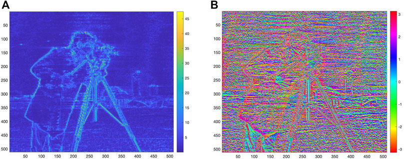
FIGURE 1. Results of CHF application on the “cameraman image” (with k = 1). In panel (A), we have the module of the CHF |h(1)|, and in panel (B), we have the associated phase ∠h(1).
Stemming on these studies on directional harmonic analysis of 2D signals, we introduce in the following sections the multiscale anisotropic harmonic filters to be adopted in the non-Euclidean manifold domain.
3 Multiscale Anisotropic Harmonic Filters
Although the HVS is very complex in nature, its low-level behavior, as determined by the primary visual cortex, is well characterized by being bandpass and orientation selective (Wu et al., 2017). Therefore, the CHF mimics these features on 2D images, and in this section, we show how to extend this behavior to manifold filters. Specifically, in this section, we describe a new class of visually driven filters operating on a manifold in the 3D space; the preliminary results on such filters appear in Conti et al.(2021). We extend the presentation in Conti et al. (2021) by an in-depth analysis of their relation with the CHF and by providing new results about their applications to point cloud filtering.
Our general idea consists in the extension of CHFs to 2D manifolds embedded in 3D domains. In this direction, the two key points to adapt to this new scenario are as follows: 1) we need to define a smoothing kernel that corresponds to the isotropic Gaussian smoothing in the 2D case; and 2) we have to identify an angular measurement on the surface of the manifold in the 3D space.
In the following sections, we elaborate on the filters description first in the case of a 2D manifold defined in a continuous 3D domain and then in the case of its discretized version, as represented by a point cloud. The main notation is reported in Table 1.

TABLE 1. Table of main notation.
3.1 MAHF on Manifolds
We first introduce the multiscale anisotropic harmonic filter (MAHF) on a continuous manifold
To this aim, we resort to the heat kernel that describes the diffusion of the heat from a point-wise source located at a point p0 on the manifold to a generic other manifold point p, after the time t. In formulas, the heat kernel
With these positions, given two points p0 and p on the manifold surface, the heat kernel is expressed as an infinite of suitable functions on the manifold. Specifically, let
The heat kernel
For what concerns angles, several definitions have been proposed in the context of convolutional neural networks on the manifold. Specifically, the polar coordinates on the geodesic can be defined using angular bins. Alternatively, a representation of points on the plane
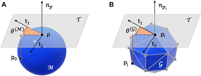
FIGURE 2. Graphical representation of angles in the 3D space. In panel (A), we represent the continuous manifold
With these positions, the multiscale anisotropic harmonic filters (MAHFs) ϕ of k order and centered in p0 are defined as follows (Conti et al., 2021):
with
3.2 MAHF on Point Clouds
In this subsection, we focus on the definition of MAHF on a 3D point cloud. Let us consider the graph
Let λn and un, n = 0, …, N − 1 denote the eigenvalues and eigenvectors of L, respectively. In this case, the heat kernel at the i-th and j-th point cloud points (pi, pj) is obtained as follows:
i.e., it depends on the weighted sum of the products of the i-th and j-th coefficients of each and every Laplacian eigenvector. The eigenvectors corresponding to small eigenvalues, i.e., the low-frequency vectors of the graph Fourier transform defined on the graph, dominate the sum for large values of the parameter t.
As the continuous case, in the discrete scenario, we define the angle
Similar to the continuous case, the multiscale anisotropic harmonic filters (MAHFs) φ of k order and centered in pi are defined as:
with
4 Visually Driven Point Cloud Filtering: MAHF as Anisotropic Analysis of Texture and Shape in Point Clouds
Let us consider a real-valued D-dimensional signal on the point cloud vertices s(pi) ∈ RD, i = 0, …, N − 1. Applying k-th-order MAHF for the vertex domain signal on graph filtering obtains the output point cloud signal r(pi) as:
The filtering realized by the MAHFs performs an anisotropic harmonic angular filtering of the signal defined on the point cloud. The period of the harmonic analysis decreases as the filter order increases, and MAHF of different orders k are matched to different angular patterns of the input signal s(pi) i = 0, …, N − 1.
MAHF applies to both texture and shape signals, depending on the choice of the input signal s(pi) i = 0, …, N − 1. For video point clouds, the signal s(pi) can represent the luminance and the chrominances observed at the point pi. If this is the case, the MAHF output highlights texture patterns on the surface. On the other hand, the signal s(pi) i = 0, …, N − 1 can be selected so as to represent geometric information. A relevant case is when the signal represents the normal to the point cloud surface at each vertex pi as follows:
The application of MAHF to the signal defined as in Eq. 8 will be exploited in the following derivation of VIPDA.
To sum up, the MAHFs can be applied to different kinds of data defined on point clouds, and they provide a way to extract several point-wise shape and texture point cloud features for different values of the order k. A schematic representation of MAHF application to texture (luminance) and shape (point cloud normals) information is illustrated in Figure 3.
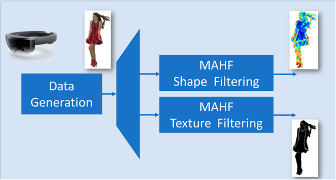
FIGURE 3. Application of MAHF to texture (luminance) and shape (point cloud normals).
5 Visually Driven Point Cloud Denoising Algorithm
In this section, we illustrate the VIPDA approach, based on application of the aforementioned MAHF to the problem of PC denoising.
Let us consider the case in which the point cloud vertices are observed in presence of an additive noise. Thereby, the observed coordinates are written as
where wi is an i.i.d. random noise. The denoising provides an estimate
Point cloud denoising algorithms typically leverage 1) data fidelity (Irfan and Magli 2021a), 2) manifold smoothness (low-rankedness) (Dinesh et al., 2020), and 3) local or cooperative averaging (Chen et al., 2019) objectives.
Here, the local manifold smoothness is accounted by adapting the estimator
Thereby, each point qi is assigned a weight related to the normal variations in its neighborhood. The key idea is that when fast variations of the normal are observed around qi, the surface smoothness is reduced, and the set of neighboring points to be exploited to compute the estimate
where
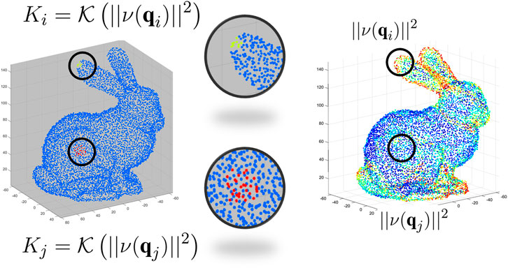
FIGURE 4. Examples of two neighborhoods of different sizes Ki and Kj (left) around points characterized by different values of the mean square value of the MAHF output ‖ν(qi)‖2 (right). The considered point cloud is a low-resolution version of the Stanford bunny in Turk and Levoy 1994).
After the size of the estimation window at each point is given, the denoising algorithm iteratively alternates 1) the computation of a candidate estimate of the point location based on spatially adaptive averaging over the Ki-size neighborhood of the i-th vertex and 2) the update of the current estimate, along the direction of the normal to the surface.
In formulas, at the l-th iteration, the candidate estimate of the i-th point cloud vertex is computed as
where η(i; Ki) denotes the set of Ki nearest neighbors of the i-th point cloud vertex. Then, the estimate is updated as
where ρ0 ∈ (0, 1] is a parameter controlling the update rate throughout the iterations. Finally, the normals
To sum up, the MAHF is applied once for all at the beginning of the iterations. For each vertex, the set of neighboring points is identified. Then, a candidate new point is computed as a weighted average of the neighbor and of the point itself. Then, the point estimated at the previous iteration is updated only by projection of the correction on the direction of the normal to the surface, as illustrated in Figure 5.
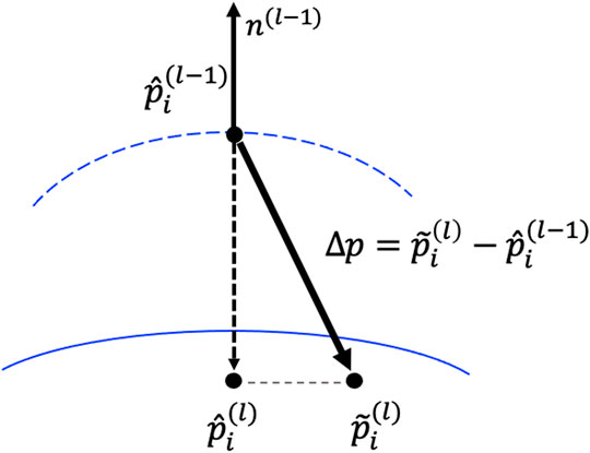
FIGURE 5. Schematic representation of the VIPDA iteration. We report the original point
The normals to the surface are recomputed. The algorithm is terminated after few iterations (1-3 in the presented simulation results).
The algorithm is summarized as follows:
Input: Noisy point clouds coordinates qi, i = 0, …, N − 1; heat kernel spread t; update rate control parameter ρ0.
Output: Denoised point clouds coordinates
Inizialization:
Computation of the heat kernel.
Computation of the normals n(0) and of their filtered version.
Computation of
Iteration: for l = 1, …, L − 1
Computation of the candidate estimate
Update of the current estimate.
Update of the normals
An overview of the VIPDA algorithm stages appears in Figure 6.
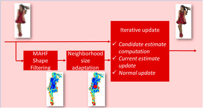
FIGURE 6. VIPDA overview.
5.1 Remarks
As far as the computational complexity of VIPDA is concerned, a few remarks are in order. First, VIPDA implies an initial MAHF-filtering stage that implies the eigendecomposition. For the computation in 5, the use of all the elements of the eigendecomposition has a really high computational cost for large N. To solve this limitation, Chebychev polynomial approximation by Huang et al. (2020); Hammond et al. (2011) can be applied in order to rewrite Eq. 5 as a polynomial in L. For the sake of concreteness, we have evaluated the time associated with each stage of the algorithm, implemented in Matlab© over a processor using this approximation for the Bunny cloud with N = 8,146. The net time for the computation of the heat kernel
Second, VIPDA is iterative, and it is not suited for parallelization. This observation stimulated the definition of an alternative version of the algorithm, namely VIPDAfast, boiling down to a single iteration and suitable for parallelization. This is achieved by a simplified application of the VIPDA key concept, that is, the adaptation of the size of the estimation neighborhood to the MAHF-filtered output. In the single iteration algorithm VIPDAfast, each point is straightforwardly estimated on a patch whose size is as a given function of the MAHF output at that point. Since all the estimates are obtained directly from the noisy sample, the algorithm may be parallelized on different subsets of points. The numerical simulation results will show that VIPDAfast, suited for parallelization, approximates the performance of the complete iterative VIPDA, especially on relatively smooth point clouds. VIPDAfast is expected to reduce the execution time in a way proportional to the number of available concurrent threads.
Finally, a remark on the noise model is in order. Indeed, the VIPDA at each iteration performs a local averaging, which tackles Gaussian noise and, in a suboptimal way, also impulsive noise. Still, the core of VIPDA allows 1) to adaptively select the neighborhood of the vertex to be used in the estimate and 2) to apply the correction to the noise component orthogonal to the mesh surface. These two principles can also be applied when the actual estimate is realized by different nonlinear operators tuned to the actual noise statistics by Ambike et al. (1994). Therefore, VIPDA can be extended to deal with different kinds of noise by replacing the average operator with a suitable nonlinear one, this is left for further study.
6 Simulation Results
In this section, we present simulation results associated with the application of MAHF on synthetic and real PC, and we measure the performances of VIPDA. In particular, in subsec.6.1, we illustrate the MAHF behavior, also in comparison with CHF, and in subsec.6.2 we assess the performance of VIPDA, also in comparison with state-of-the-art denoising algorithms.
6.1 MAHF-Based Point Cloud Filtering
In this subsection, we present some examples on the application of MAHF on different point clouds. In this article, we introduce a point cloud filtering method inspired by HVS, and we show its potential to both geometric and texture PC data. The proposed class of filters presents a local anisotropic behavior that highlights directional components of the point cloud texture or geometry. The filter output can be leveraged as input to various adaptive processing tasks.
First, we consider the case of a point cloud obtained by equispaced sampling of a planar surface, over which a discontinuous signal is defined. This case is illustrated in Figure 7A), in which we see the point cloud in which a two-valued signal is defined; the signal is characterized by a discontinuity in the middle. Then, MAHF filtering (with k = 1) is applied. In Figure 7B, we report the square of the module of the related MAHF output. As expected, the MAHF highlights the vertices in correspondence with the signal discontinuity. In order to compare MAHF with CHF behavior, we take into account an analogous scenario for CHF filtering, namely we consider an image representing a discrete bidimensional step function, which is represented in Figure 8A. We apply the k = 1 CHF to the image, and we separately plot its module and phase in the panel Figures 8B, C, respectively. The output of the k = 1 MAHF and CHF filters highlights the areas in correspondence with the discontinuity of the signal. Thereby, we recognize that the k = 1 MAHF filter straightforwardly extends to the planar point cloud domain, the behavior observed applying the k = 1 CHF filter on image data. Indeed, we remark that the MAHF and CHF filters definitions in the point cloud domain and image domain, respectively, are analogous, and it is expected that the MAHF can retrieve structured discontinuities of the signals defined on a point cloud.
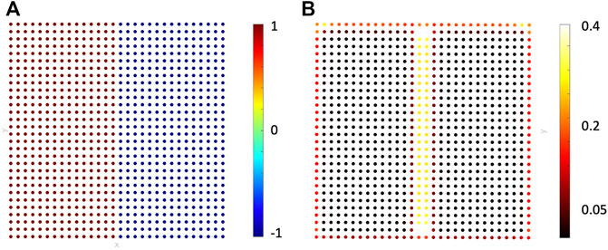
FIGURE 7. Results of the application of MAHF (k = 1) on a two-valued signal (in panel (A)). We compute the MAHF, and we report the square of the module of the output in panel (B).
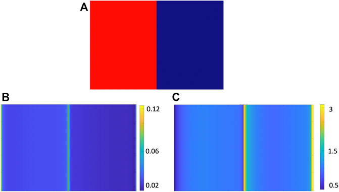
FIGURE 8. Results of the application of CHF (k = 1) on a discrete bidimensional step function in panel (A). We compute the output of the MAHF, and we report the square of the module in panel (B) and the phase in panel (C).
After exemplifying the relation between MAHF and CHF, we apply MAHF to open access point clouds. For this study, we consider two point clouds belonging to the 8iVSLF dataset (d’Eon et al., 2017). Specifically, we consider the point clouds red and black and long dress (d’Eon et al., 2017), which are the 3D point clouds illustrated in the insets of panels A and B in Figure 9. Each point cloud vertex is associated to the red, green, and blue components of the surface color as seen using a multi-camera rig. The original point clouds red and black and long dress have been resampled to a number of points equal to N = 9,622 and N = 9,378, respectively.
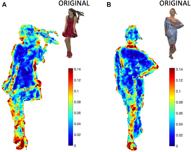
FIGURE 9. MAHF applied on the point cloud normals for different data: (A) red and black and (B) long dress. In the insets of each panel, we have original images. Here, MAHFs are applied to the normals
First of all, we apply MAHF to the normals
Then, for each point cloud, we analyze the filtering of the color information. At each vertex pi, i = 0, …, N − 1, we compute the luminance given by the available RGB values, and we apply MAHF by considering the luminance as the real-valued input signal s(pi), i = 0, …, N − 1 over the point cloud graph. The MAHF output
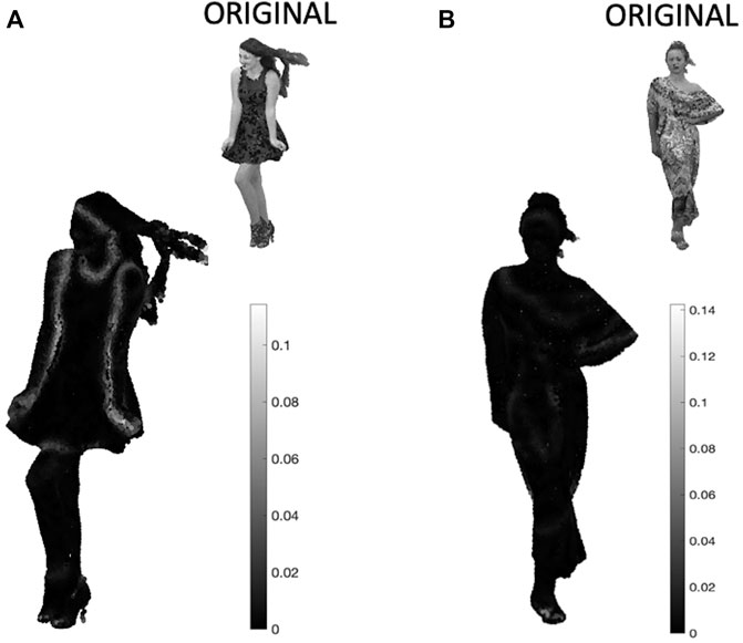
FIGURE 10. MAHF applied on luminance images for two point clouds: (A) red and black and (B) long dress. We report the original luminance images in the insets of each panel. In this case, MAHFs are applied to the luminance s(pi). We compute the square module of the MAHF output, which corresponds to r(pi).
6.2 VIPDA Performances
After illustrating the application of MAHF to point cloud filtering on shape and texture information by means of examples on real data, we address the assessment of VIPDA in this subsection.
To this aim, we first illustrate the application of VIPDA over synthetic data. Specifically, we consider the point cloud related to the Stanford bunny (Turk and Levoy 1994), resampled at N = 8,146. The noisy coordinates qi of the points on the PC are obtained as in Eq. 9. In the simulations, a Gaussian noise wi is added to the original coordinates pi. The intensity of the additive noise is measured by the signal-to-noise ratio (SNR), which is a parameter varied in the following analyses, and it is computed as:
We plot the original point cloud in Figure 11A, in which the pseudo-color is associated to the third coordinate of qi, i = 0, …, N − 1 (coordinate w.r.t. the z-axis). In Figure 11B, we plot the noisy point cloud obtained for SNRnoisy = 38dB. The pseudo-colors of the point cloud represent the square module of the difference between the noisy coordinates ‖pi − qi‖2, i = 0, …, N − 1 and the original ones computed as ‖pi − qi‖2. In this manner, the point color (represented in a color scale from blue for zero values and red for the maximum values) reflects how much each point is corrupted by the additive Gaussian noise.
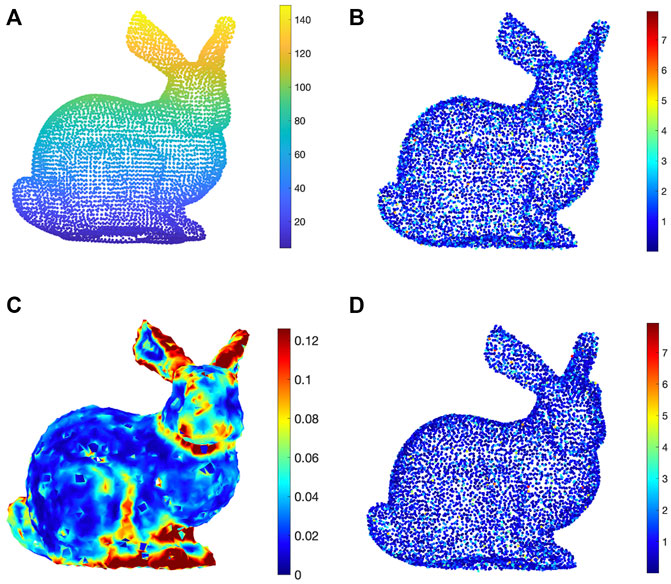
FIGURE 11. Results of VIPDA at each step. We consider a point cloud related to the Stanford bunny (Turk and Levoy 1994) which is represented with its original coordinates pi in panel (A). Then, a Gaussian noise wi is added with SNR = 38, and the noisy points qi on the point cloud are represented in panel (B). The colors associated to the color bar correspond to the difference between noisy and original coordinates ‖pi − qi‖2. In panel (C), we report the output of the MAHF ‖ν(qi)‖2 applied to the estimated normals
Then, we apply the MAHF to the estimated normals n(qi), i = 0, …, N − 1 of the noisy point cloud, and we compute the square value of the MAHF output at each vertex, namely ‖ν(qi)‖2, i = 0, …, N − 1. The so-obtained values are illustrated in Figure 11C, as pseudo-colors at the vertices. We recognize that the largest values are observed in correspondence to vertices in areas of normal changes. These results exemplify that the MAHFs are able to capture the variability of the signals.
Finally, we apply VIPDA to the filtered point cloud, and we show the denoised point cloud in Figure 11D. Here, we have the
Specifically, we design a signal-dependent feature graph Laplacian regularizer (SDFGLR) that assumes surface normals computed from point coordinates are piecewise smooth with respect to a signal-dependent graph Laplacian matrix.
Finally, we perform analyses based on the SNR and compare our method with different alternatives. In this direction, we first consider the algorithm proposed in Dinesh et al., (2020), in which authors perform a graph Laplacian regularization that starts from the hypothesis that the normals to the surface at the point cloud vertices are smooth w.r.t graph Laplacian. For sake of comparison, we also study the average case, in which we analyze the PC results from the local average of its spatial coordinates. Finally, we consider the VIPDA and the VIPDAfast algorithms. In the simulations,
In order to perform the computations, we first consider the Stanford bunny point cloud, and we select different levels of SNR, namely SNRnoisy = 35, 38, 40, 48dB. Then, we take into account different denoising algorithms and report the SNR achieved on the denoised point cloud in Table 2. For each method, we compute the SNR as the distance between the reconstructed coordinates and the original ones as
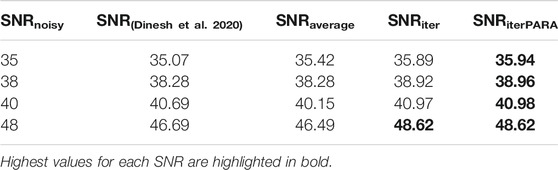
TABLE 2. Table of SNR with Stanford bunny point cloud.
Our results show that our denoising method outperforms the alternatives. The method with the parallelization even increases the performances w.r.t. the iterative one. This is due to the particular nature of the point cloud, in which the flat areas and the high curvature areas are relatively easy to distinguish, and the method coarsely operating on the two point sets achieves the best results. This is more clearly highlighted on point clouds acquired on real objects as illustrated in the following: We consider the two other point clouds (Red and Black and Long Dress) for two fixed levels of noise with SNR at 40dB and 48dB. The results are, respectively, reported in Tables 3, 4. SNR values show that the proposed VIPDA, either in its original or fast version, performs better than state-of-the-art competitors in denoising point cloud signals corrupted by Gaussian noise. Finally, we consider a smooth point cloud, namely a sphere with N = 900 points. Also on this smooth point cloud, where the MAHF gives a uniform output and the patch size is fixed, VIPDA achieves an SNR improvement. The correction by VIPDA is restrained to the normal direction and leads to a smooth surface. Thereby, VIPDA achieves a SNR improvement also on smooth surfaces, and an improvement due to the reduction of the normal noise component is observed even in the limit case of a planar mesh.
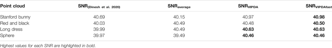
TABLE 3. Table of SNR with fixed SNR of noisy data at 40 dB with different point clouds, i.e., Stanford bunny, long dress and red and black, and spherical meshes.
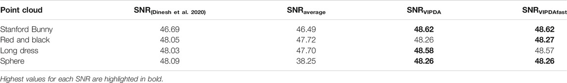
TABLE 4. Table of SNR with fixed SNR of noisy data at 48 dB with several point clouds, i.e., Stanford bunny, long dress and red and black, and spherical meshes.
It is important to mention that the performance of all the methods, including the proposed method, degrades severely if the SNR decreases. This is due to the fact that, in correspondence with low SNR, the positions of the vertices are displaced such that the positions of the noisy points may even exchange with respect to the original ones, and this phenomenon is not recovered even though the MAHF on the signal is recomputed at each iteration. A possible solution to this would be to initially denoise the Laplacian associated to the point cloud graph by leveraging a spectral prior, as in Cattai et al. (2021), or by jointly exploiting the shape and texture information; this latter point is left for future studies.
To sum up, these findings demonstrate the potential of the proposed VIPDA approach for point cloud denoising and pave the way for designing new processing tools for signals defined over non-Euclidean domains.
7 Conclusion
This work has presented a novel point cloud denoising approach, the visually driven point cloud denoising algorithm (VIPDA). The proposed method differs from other competitors in linking the denoising with visually relevant features, as estimated by suitable anisotropic angular filters in the vertex domain.
VIPDA leverages properties inspired by those of the human visual system (HVS), and it is viable for application on the texture and geometry data defined over a point cloud. The VIPDA approach leads to smooth denoised surfaces since it iteratively corrects the noise component normal to the manifold underlying the point cloud by projecting the observed noisy vertex toward the plane tangent to the underlying manifold surface. The performance of VIPDA has been numerically assessed on real open access data and compared with state-of-the-art alternatives.
The proposed algorithm is effective in denoising real point cloud data, and thereby it makes point cloud modeling more suitable for real applications. Our findings pave the way to HVS-inspired point cloud processing, both for enhancement and restoration purposes, by suitable anisotropic angular filtering.
Data Availability Statement
Publicly available datasets were analyzed in this study. These data can be found at: https://mpeg-pcc.org/index.php/pcc-content-database/.
Author Contributions
TC and SC conceived and designed the analysis; AD collected the data, performed the analysis, and contributed to the algorithm definition; GS contributed to the analysis tools; and TC and SC wrote the manuscript.
Conflict of Interest
The authors declare that the research was conducted in the absence of any commercial or financial relationships that could be construed as a potential conflict of interest.
Publisher’s Note
All claims expressed in this article are solely those of the authors and do not necessarily represent those of their affiliated organizations, or those of the publisher, the editors, and the reviewers. Any product that may be evaluated in this article, or claim that may be made by its manufacturer, is not guaranteed or endorsed by the publisher.
Footnotes
1Let Δ denote the Laplace–Bertrami operator, i.e., a linear operator computing the sum of directional derivatives of a function defined on the manifold. The heat propagation equation is written as:
where f(p, t) is the solution under initial condition f0(p).
2The point cloud normals are computed using the ©Matlab by the implementation of the method in Hoppe et al. (1992).
References
Ambike, S., Ilow, J., and Hatzinakos, D. (1994). Detection for Binary Transmission in a Mixture of Gaussian Noise and Impulsive Noise Modeled as an Alpha-Stable Process. IEEE Signal. Process. Lett. 1, 55–57. doi:10.1109/97.295323
Beghdadi, A., Larabi, M.-C., Bouzerdoum, A., and Iftekharuddin, K. M. (2013). A Survey of Perceptual Image Processing Methods. Signal. Processing: Image Commun. 28, 811–831. doi:10.1016/j.image.2013.06.003
Belkin, M., Sun, J., and Wang, Y. (2009). “Constructing Laplace Operator from point Clouds in Rd,” in Proceedings of the Twentieth Annual ACM-SIAM Symposium on Discrete Algorithms, New York, January 4–6, 2009 (SIAM), 1031–1040.
Campisi, P., and Scarano, G. (2002). A Multiresolution Approach for Texture Synthesis Using the Circular Harmonic Functions. IEEE Trans. Image Process. 11, 37–51. doi:10.1109/83.977881
Cattai, T., Scarano, G., Corsi, M.-C., Bassett, D., De Vico Fallani, F., and Colonnese, S. (2021). Improving J-Divergence of Brain Connectivity States by Graph Laplacian Denoising. IEEE Trans. Signal. Inf. Process. Over Networks 7, 493–508. doi:10.1109/tsipn.2021.3100302
Chen, H., Wei, M., Sun, Y., Xie, X., and Wang, J. (2019). Multi-patch Collaborative point Cloud Denoising via Low-Rank Recovery with Graph Constraint. IEEE Trans. Vis. Comput. Graph 26, 3255–3270. doi:10.1109/TVCG.2019.2920817
Chen, H., Xu, F., Liu, W., Sun, D., Liu, P. X., Menhas, M. I., et al. (2021). 3d Reconstruction of Unstructured Objects Using Information from Multiple Sensors. IEEE Sensors J. 21–26963. doi:10.1109/jsen.2021.3121343.26951
Colonnese, S., Campisi, P., Panci, G., and Scarano, G. (2004). Blind Image Deblurring Driven by Nonlinear Processing in the Edge Domain. EURASIP J. Adv. Signal Process. 2004, 1–14. doi:10.1155/s1110865704404132
Colonnese, S., Randi, R., Rinauro, S., and Scarano, G. (2010). “Fast Image Interpolation Using Circular Harmonic Functions,” in 2010 2nd European Workshop on Visual Information Processing (EUVIP), Paris, France, 5–7 July 2010 (IEEE), 114–118. doi:10.1109/euvip.2010.5699119
Colonnese, S., Rinauro, S., and Scarano, G. (2013). Bayesian Image Interpolation Using Markov Random fields Driven by Visually Relevant Image Features. Signal. Processing: Image Commun. 28, 967–983. doi:10.1016/j.image.2012.07.001
Conti, F., Scarano, G., and Colonnese, S. (2021). “Multiscale Anisotropic Harmonic Filters on Non Euclidean Domains,” in 2021 29th European Signal Processing Conference (EUSIPCO) (Virtual Conference), (IEEE), 701–705.
d’Eon, E., Harrison, B., Myers, T., and Chou, P. A. (2017). 8i Voxelized Full Bodies-A Voxelized point Cloud Dataset. ISO/IEC JTC1/SC29 Joint WG11/WG1 (MPEG/JPEG) input document WG11M40059/WG1M74006 7, 8
Dai, Y., Wen, C., Wu, H., Guo, Y., Chen, L., and Wang, C. (2021). “Indoor 3d Human Trajectory Reconstruction Using Surveillance Camera Videos and point Clouds,” in IEEE Transactions on Circuits and Systems for Video Technology. doi:10.1109/tcsvt.2021.3081591
de Hoog, J., Ahmed, A. N., Anwar, A., Latré, S., and Hellinckx, P. (2021). “Quality-aware Compression of point Clouds with Google Draco,” in Advances on P2P, Parallel, Grid, Cloud and Internet Computing. 3PGCIC 2021. Lecture Notes in Networks and Systems. Editor L. Barolli (Cham: Springer) 343, 227–236. doi:10.1007/978-3-030-89899-1_23
Dinesh, C., Cheung, G., and Bajic, I. V. (2020). Point Cloud Denoising via Feature Graph Laplacian Regularization. IEEE Trans. Image Process. 29, 4143–4158. doi:10.1109/tip.2020.2969052
Diniz, R., Farias, M. Q., and Garcia-Freitas, P. (2021). “Color and Geometry Texture Descriptors for point-cloud Quality Assessment,” in IEEE Signal Processing Letters. doi:10.1109/lsp.2021.3088059
Erçelik, E., Yurtsever, E., and Knoll, A. (2021). 3d Object Detection with Multi-Frame Rgb-Lidar Feature Alignment. IEEE Access 9, 143138–143149. doi:10.1109/ACCESS.2021.3120261
Friedlander, B. (1984). On the Cramer- Rao Bound for Time Delay and Doppler Estimation (Corresp.). IEEE Trans. Inform. Theor. 30, 575–580. doi:10.1109/tit.1984.1056901
Hammond, D. K., Vandergheynst, P., and Gribonval, R. (2011). Wavelets on Graphs via Spectral Graph Theory. Appl. Comput. Harmonic Anal. 30, 129–150. doi:10.1016/j.acha.2010.04.005
Hoppe, H., DeRose, T., Duchamp, T., McDonald, J., and Stuetzle, W. (1992). Surface Reconstruction from Unorganized Points. ACM SIGGRAPH Comput. Graph. 26, 71–78. doi:10.1145/142920.134011
Hou, T., and Qin, H. (2012). Continuous and Discrete Mexican Hat Wavelet Transforms on Manifolds. Graphical Models 74, 221–232. doi:10.1016/j.gmod.2012.04.010
Hu, W., Hu, Q., Wang, Z., and Gao, X. (2021a). Dynamic point Cloud Denoising via Manifold-To-Manifold Distance. IEEE Trans. Image Process. 30, 6168–6183. doi:10.1109/tip.2021.3092826
Hu, W., Pang, J., Liu, X., Tian, D., Lin, C.-W., and Vetro, A. (2021b). “Graph Signal Processing for Geometric Data and beyond: Theory and Applications,” in IEEE Transactions on Multimedia. doi:10.1109/tmm.2021.3111440
Huang, J., Choudhury, P. K., Yin, S., and Zhu, L. (2021). Real-time Road Curb and Lane Detection for Autonomous Driving Using Lidar point Clouds. IEEE Access 9, 144940–144951. doi:10.1109/access.2021.3120741
Huang, S.-G., Lyu, I., Qiu, A., and Chung, M. K. (2020). Fast Polynomial Approximation of Heat Kernel Convolution on Manifolds and its Application to Brain Sulcal and Gyral Graph Pattern Analysis. IEEE Trans. Med. Imaging 39, 2201–2212. doi:10.1109/tmi.2020.2967451
Huang, T., Li, R., Li, Y., Zhang, X., and Liao, H. (2021). Augmented Reality-Based Autostereoscopic Surgical Visualization System for Telesurgery. Int. J. Comput. Assist. Radiol. Surg. 16, 1985–1997. doi:10.1007/s11548-021-02463-5
Irfan, M. A., and Magli, E. (2021a). Exploiting Color for Graph-Based 3d point Cloud Denoising. J. Vis. Commun. Image Representation 75, 103027. doi:10.1016/j.jvcir.2021.103027
Irfan, M. A., and Magli, E. (2021b). Joint Geometry and Color point Cloud Denoising Based on Graph Wavelets. IEEE Access 9, 21149–21166. doi:10.1109/access.2021.3054171
Jacovitti, G., and Neri, A. (2000). Multiresolution Circular Harmonic Decomposition. IEEE Trans. Signal. Process. 48, 3242–3247. doi:10.1109/78.875481
Ji, T., Guo, Y., Wang, Q., Wang, X., and Li, P. (2021). Economy: Point Clouds-Based Energy-Efficient Autonomous Navigation for Uavs. IEEE Trans. Netw. Sci. Eng. 8 (4), 2885–2896. doi:10.1109/tnse.2021.3049263
Neri, A., and Jacovitti, G. (2004). Maximum Likelihood Localization of 2-d Patterns in the Gauss-Laguerre Transform Domain: Theoretic Framework and Preliminary Results. IEEE Trans. Image Process. 13, 72–86. doi:10.1109/tip.2003.818021
Panci, G., Campisi, P., Colonnese, S., and Scarano, G. (2003). Multichannel Blind Image Deconvolution Using the Bussgang Algorithm: Spatial and Multiresolution Approaches. IEEE Trans. Image Process. 12, 1324–1337. doi:10.1109/tip.2003.818022
Ramalho, E., Peixoto, E., and Medeiros, E. (2021). Silhouette 4d with Context Selection: Lossless Geometry Compression of Dynamic point Clouds. IEEE Signal. Process. Lett. 28, 1660–1664. doi:10.1109/lsp.2021.3102525
Rist, C., Emmerichs, D., Enzweiler, M., and Gavrila, D. (2021). “Semantic Scene Completion Using Local Deep Implicit Functions on Lidar Data,” in IEEE Transactions on Pattern Analysis and Machine Intelligence. doi:10.1109/tpami.2021.3095302
Sun, X., Wang, S., Wang, M., Cheng, S. S., and Liu, M. (2020). “An Advanced Lidar point Cloud Sequence Coding Scheme for Autonomous Driving,” in Proceedings of the 28th ACM International Conference on Multimedia, Seattle, WA, USA, October 12–16, 2020, 2793–2801. doi:10.1145/3394171.3413537
Turk, G., and Levoy, M. (1994). “Zippered Polygon Meshes from Range Images,” in Proceedings of the 21st annual conference on Computer graphics and interactive techniques, Orlando, Florida, July 24–29, 1994. Computer Graphics Proceedings, Annual Conference Series (ACM SIGGRAPH), 311–318. doi:10.1145/192161.192241
Wu, J., Li, L., Dong, W., Shi, G., Lin, W., and Kuo, C.-C. J. (2017). Enhanced Just Noticeable Difference Model for Images with Pattern Complexity. IEEE Trans. Image Process. 26, 2682–2693. doi:10.1109/tip.2017.2685682
Xiong, J., Gao, H., Wang, M., Li, H., and Lin, W. (2021). “Occupancy Map Guided Fast Video-Based Dynamic point Cloud Coding,” in IEEE Transactions on Circuits and Systems for Video Technology.
Yang, Q., Ma, Z., Xu, Y., Li, Z., and Sun, J. (2020). “Inferring point Cloud Quality via Graph Similarity,” in IEEE Transactions on Pattern Analysis and Machine Intelligence.
Yu, K., Gorbachev, G., Eck, U., Pankratz, F., Navab, N., and Roth, D. (2021). Avatars for Teleconsultation: Effects of Avatar Embodiment Techniques on User Perception in 3d Asymmetric Telepresence. IEEE Trans. Vis. Comput. Graphics 27, 4129–4139. doi:10.1109/tvcg.2021.3106480
Keywords: point cloud, denoising, non-Euclidean domain, angular harmonic filtering, graph signal processing
Citation: Cattai T, Delfino A, Scarano G and Colonnese S (2022) VIPDA: A Visually Driven Point Cloud Denoising Algorithm Based on Anisotropic Point Cloud Filtering. Front. Sig. Proc. 2:842570. doi: 10.3389/frsip.2022.842570
Received: 23 December 2021; Accepted: 15 February 2022;
Published: 16 March 2022.
Edited by:
Hagit Messer, Tel Aviv University, IsraelReviewed by:
Milos Brajovic, University of Montenegro, MontenegroMiaohui Wang, Shenzhen University, China
Copyright © 2022 Cattai, Delfino, Scarano and Colonnese. This is an open-access article distributed under the terms of the Creative Commons Attribution License (CC BY). The use, distribution or reproduction in other forums is permitted, provided the original author(s) and the copyright owner(s) are credited and that the original publication in this journal is cited, in accordance with accepted academic practice. No use, distribution or reproduction is permitted which does not comply with these terms.
*Correspondence: Stefania Colonnese, c3RlZmFuaWEuY29sb25uZXNlQHVuaXJvbWExLml0