How Scalable Are Clade-Specific Marker K-Mer Based Hash Methods for Metagenomic Taxonomic Classification?

Efficiently and accurately identifying which microbes are present in a biological sample is important to medicine and biology. For example, in medicine, microbe identification allows doctors to better diagnose diseases. Two questions are essential to metagenomic analysis (the analysis of a random sampling of DNA in a patient/environment sample): How to accurately identify the microbes in samples and how to efficiently update the taxonomic classifier as new microbe genomes are sequenced and added to the reference database. To investigate how classifiers change as they train on more knowledge, we made sub-databases composed of genomes that existed in past years that served as “snapshots in time” (1999–2020) of the NCBI reference genome database. We evaluated two classification methods, Kraken 2 and CLARK with these snapshots using a real, experimental metagenomic sample from a human gut. This allowed us to measure how much of a real sample could confidently classify using these methods and as the database grows. Despite not knowing the ground truth, we could measure the concordance between methods and between years of the database within each method using a Bray-Curtis distance. In addition, we also recorded the training times of the classifiers for each snapshot. For all data for Kraken 2, we observed that as more genomes were added, more microbes from the sample were classified. CLARK had a similar trend, but in the final year, this trend reversed with the microbial variation and less unique k-mers. Also, both classifiers, while having different ways of training, generally are linear in time - but Kraken 2 has a significantly lower slope in scaling to more data.

Background

DNA sequencing has enabled the investigation of microbial communities using cultivation-independent, DNA/RNA-based approaches (Brul et al., 2010; Berg et al., 2020; Coenen, 2020). We can think of these microbial communities as microscopic civilizations, in which bacteria not only act independently but learn to cooperate and compete with each other, to gain more nutrients and resources, and that result in advanced time-course patterns of microbial proliferation and death (Figueiredo et al., 2020). As humans, we must take observations of microbiomes. While imaging is still too coarse for observing 10¹¹ cells per Gram of colon content (Sender et al., 2016), sampling their DNA from next-generation sequencing of microbes is commonly used, with many other ‘omic techniques emerging that sample measurements of the metatranscriptome, metaproteome, and metabolome (Creasy et al., 2021). Microbiomes are found everywhere on Earth, including soil, water, air, and animal hosts (Nemergut et al., 2013). Understanding microbiomes is the first step, with many potential engineering applications to follow (Woloszynek et al., 2016).

Signal processing has played an important role in metagenomic identification and taxonomic classification, which is the supervised labeling of a taxonomic class to a DNA/RNA sequencing read (Rosen and Moore, 2003; Rosen et al., 2009; Borrayo, 2014; Alshawaqfeh, 2017; Elworth et al., 2020). While taxonomic classification is the application that we cover in this paper, metagenomics is not limited only to this problem, and emerging techniques are proving useful for unsupervised “binning” of metagenomics reads (Kouchaki et al., 2019). Information-theoretic feature selection (Garbarine et al., 2011) and deep neural network sequence embeddings (Woloszynek et al., 2019), useful methods from signal processing, can be performed before metagenomic taxonomic classification to reduce feature dimensionality and computational complexity.

As of 2019, over 80 metagenomic taxonomic classification tools have been published (Gardner et al., 2019), while benchmarking efforts try to quantify the most representative ones (Ye et al., 2019). We have previously shown an in-depth case study of the naïve Bayes classifier’s (and its incremental version’s) accuracy and speed over the yearly growth of NCBI (Zhao et al., 2020). Now, for this study, we study clade-specific marker hash-based techniques, due to their popularity, efficiency/speed, and comparable sensitivity/precision when benchmarked against BLAST-based methods (Wood et al., 2014). These algorithms have been shown to be competitive algorithms on several benchmarks on real and simulated data (McIntyre et al., 2017; Sczyrba et al., 2017; Meyer et al., 2021). In 2017, a comparison of the two algorithms shows their performances are relatively similar, with CLARK tending to yield better relative abundance estimates than Kraken2, which can be due to more genomes in their curated database (McIntyre et al., 2017). While there are techniques like sourmash (Brown and Irber, 2016; Liu and Koslicki, 2022; LaPierre et al., 2020) that can sketch k-mer compositions, they do not perform well when the reference genome is missing from the database (dibsi-rnaseq, 2016). While Kraken2/CLARK has been shown to predict low-abundance false positives, it has been shown that a larger database can improve Kraken2 performance (LaPierre et al., 2020). Other techniques, such as LSHvec (Shi and Chen, 2021), which embeds sequences after a compression k-mers with a hash, may be able to transform the some of the limitations of hash-based techniques using deep learning. Therefore, LaPierre et al. and McIntyre et al.‘s study invite an investigation into how database composition can affect methods that use these efficient k-mer presence/absence to differentiate clades, and this study can give insight into how more recent hash-based techniques will perform.

It has been previously shown that database size influences the accuracy of Kraken and its Bayesian extension Bracken (Nasko et al., 2018). While the study highlights the percentage of “unclassified” reads goes down as the database grows, it does not fully examine time to run the algorithms over varying size databases or how the final relative abundance result changes. As genomes in the databases increase, the representation of the organisms in the database may not always be uniform across the tree of life. With mutations, clade-identifying k-mers that may have been previously discriminating between taxa before, may be missing in updates, reducing the search capacity of these methods. These identifying k-mers will not be captured simply by looking at orthologs shared between genomes (Lan et al., 2014). Therefore, the size of the database and its growth may affect performance of the kmer-based algorithms in addition to runtime.

CLARK and Kraken 2

CLARK and Kraken 2 are both well known metagenomic classifiers, software that “reads” short sequences of DNA and attempts to accurately identify what organism they came from. Although CLARK and Kraken 2 are both clade-specific k-mer hash-based metagenomic classifiers, they operate in different, almost opposite, ways. Both software, like most classifiers, decompose the DNA sequences into smaller features called k-mers to make comparisons easier. Their k-mers are 31 nucleotides long by default. CLARK’s training step takes each k-mer and cycles through all the genomes in its database to see if any of them have that sequence. If more than one genome does, then the k-mer is ignored and the program moves on to the next one. Now when a query sequence is tested, for each k-mer in the query, if only one genome matches it, then that genome’s score of how many k-mers it matches the query is incremented. This approach prioritizes the calculation of unique k-mers, or k-mers that are only found in one genome to the query. After all the k-mers are cycled through, the genome with the highest unique k-mer score is deemed as the correct match. If the score is too low or there are genomes that tie, then the sample DNA is marked as unclassified (Ounit et al., 2015).

On the other hand, when Kraken 2 compares a k-mer in the query to the genomes in its database, for any k-mer match, the genome score is incremented by one. Kraken 2 doesn’t skip over k-mers that are shared by multiple genomes (Wood et al., 2014). Instead, it takes those into account. This approach prioritizes common k-mers, specifically the k-mers that the genomes have in common with the query DNA. The genome with the highest common k-mer score is deemed the correct match. In the event of a tie or if the scores do not meet Kraken 2’s default threshold (the genome has a confidence threshold of 0.65), then the sample DNA is marked as unclassified (Wood et al., 2019).

Goals

The goals of this paper are to examine the behaviors of metagenomic classifiers as the information in their databases increases over time: how much they classify, how they classify, and how fast they classify. While similar studies have been previously conducted, they are for other methods and for the study of Kraken 2, it was limited. For example, Nasko et al. (2018) examined Kraken’s performance for successive Refseq databases, but the metrics were mostly for speed and amount classified (but not how the distribution of those classified changed). We wish to gain a more comprehensive insight into the scalability of k-mer based hash methods of metagenomic classifiers. We also wanted to compare two well-known classifiers, CLARK and Kraken 2, to see which one was more efficient and how both of them could improve to be useful into the future as more genomes are sequenced and added to their databases. Also, we previously benchmarked the naive Bayes classifier (Zhao et al., 2020) for its accuracy to classify (NBC classifies everything so the “amount” is negligible) and speed, and we will use the same dataset (devised on a yearly basis) in this study so that it can be fairly compared.

Methodology

Datasets

The build/train (sub-)databases are derived from the National Center for Biotechnology Information (NCBI) Reference Sequence (RefSeq) bacterial genome database (Sayers et al., 2019) and the NCBI genbank assembly summary file for bacteria available at ftp://ftp.ncbi.nlm.nih.gov/genomes/genbank/bacteria/assembly_summary.txt. The test data is taken from NCBI’s Sequence Read Archive (SRA ID: SRS105153) (Huttenhower et al., 2012) and is a human gut sample from the Human Microbiome Project (Nasko et al., 2018). We use experimental data because it is more likely to contain a true distribution of novel taxa.

Setup, Build, and Classify

The database snapshots from 1999 to 2020 were designed in (Zhao et al., 2020). Statistics about the database growth in genomes and their lineages can be found in that paper’s Additional File 1: https://www.ncbi.nlm.nih.gov/pmc/articles/PMC7507296/bin/12859_2020_3744_MOESM1_ESM.pdf. The genomes from these lists were obtained in Kraken and usually a subset was found in CLARK’s downloaded database. In the supplementary additional file 2, we provide the Kraken/CLARK overlap and the additional genomes in Kraken (that were not found in CLARK’s database).

Kraken 2

Kraken 2’s default bacteria database was used to find the list of bacteria genomes. All uncompleted genomes were filtered out, leaving only the completed ones left in the list. Six lists (1999, 2004, 2009, 2014, 2019, and 2020) were then created, as shown in Figure 1. Each was filled with genomes that were sequenced in their respective years or before. For example, A bacteria genome sequenced in 2010 would be in the 2014, 2019, and 2020 list, but a genome sequenced in 2020 would only be present in the 2020 list. For Kraken 2, those genome lists were then used to create library. fna files that Kraken 2 uses in its databases (Wood et al., 2014). Those library. fna files were then used to create six sub-databases for Kraken 2 (1999, 2004, 2009, 2014, 2019, and 2020).

FIGURE 1

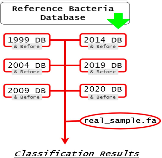
FIGURE 1. A proof-of-concept diagram for your reference.

Creating the custom library. fna files required python programs: summary. py and hive. py. After this set up, each Kraken 2 sub-database was built and used to classify SRA ID: SRS105153, a file containing about 70 million reads (approximately 100-200bp in length per read) from a human gut sample (Huttenhower et al., 2012).

CLARK

CLARK’s custom sub-databases were built with the same lists as in Figure 1, but in a slightly different way. The difference is in how CLARK stored its genomes. When CLARK’s default bacteria database was downloaded, the genomes were stored in individual FASTA files. Some files had more than one genome written in it, but each file’s name corresponded to a GCF accession code. This made sorting the genomes from the default bacteria database into the custom databases much easier. After finding all the file paths for each of the GCF accession numbers, those files would then be copied into the “Custom/” folder of their corresponding custom sub-database.

${\mathit{T}}_{\mathit{CB}}={\mathit{T}}_{\mathit{B}}+\left({\mathit{C}}_{\mathit{R}\mathbf{1}}-\mathit{ }{\mathit{C}}_{\mathit{R}\mathbf{2}}\right)(1)$

Where TBC is the entire CLARK build time, TB is the runtime of the initial stage of the build/training time of CLARK. It is then added to the second stage of the build time which is calculated by subtracting first run (which is the first stage build + classify times), CR1, minus solely the classify times, CR2. CR1 is the runtime for CLARK’s classification script “classify_metagenomes.sh” when it is run with a particular database for the first time, and CR2 is the runtime for CLARK’s classification script when it is run on that same database after the first time (second, third, etc. time).

Building a database with CLARK is not as straightforward as with Kraken 2. CLARK does its database building in two parts: the first part with its actual building script and the second part is built when the database is first used during classification. CLARK also does not store the built database in a directory. Instead, if you want to use a different database or previous database, the build script must be run again, which includes both a build component and a classify component. Due to this combination of steps in the script, CLARK’s build time was calculated (Eq. (1)). This was done by subtracting the second classification runtime (where only classification occurred) from the first (where the second part of database building was done). That difference was then added to the runtime of the build script (the first part of the building) to get the full runtime of CLARK’s database building.

Parsing the Results

Kraken 2

For the Kraken 2 classification results, the text files were parsed line by line to gather information on whether that read was classified and what it was classified as. This information was stored into a Python dictionary, as well as a count variable that kept track of how many reads were classified as a particular taxa or how many were unclassified (Figure 2). Traceback was also performed to include counts of every taxonomic rank. For example, if a read was classified as genus X, then genus X’s family, class, order, etc. would also be counted.

FIGURE 2

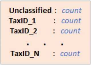
FIGURE 2. The taxa in CLARK and Kraken 2’s results and the number of reads that were classified as that taxa (count).

CLARK

Since CLARK’s classification results were stored in. csv files, they were easy to parse. Each row in the “Assignment” column was read to ascertain what CLARK classified the read as. Traceback was also performed here, and the information was stored the same way Kraken 2’s was (Figure 2).

Relative Abundance, Triangular Bray-Curtis, and Graphing

Calculating Relative Abundance

$R{A}_i= \frac{C_i}{{{\displaystyle \sum }}_i{C}_i} \times 100\%(2)$

where $R{A}_i$ is the relative abundance for a particular taxonomic class i. $C_i$ is the number of times that a DNA read from class i is observed in the sample divided by the number of all observations (DNA reads) from all classes.

A general equation (Eq. 2) was used to calculate each taxa’s relative abundance in two different ways. The first way was to calculate the taxa’s relative abundance within the set of reads that were given a classification label. This means that each read was assigned one of {C₀, C₁, ..., C_N-1}, where N is the number of taxonomic units in a given taxonomic rank in the classification results, and summed then divided by the total reads on the taxonomic level (e.g. on the species level, each species is incremented by the count of each read assigned to that species and then divided by the total reads that classify on the species level). In other words, the count of each taxa was divided by the total number of classified reads, then multiplied by 100 to make it a percentage.

The second way was to calculate the taxa’s relative abundance among the total number of reads. To illustrate the labeling of all reads, an unclassified category was added such that i ∈ {I, … , N, unclassified} so that C_unclassified is accounted for as a bar in the graph and in the denominator of the relative abundance calculation. These results were exported to excel file sheets for each taxonomic rank.

Graphing Relative Abundance

Each taxa’s relative abundance is compared to a 3% threshold, meaning that any taxa that has a relative abundance above 3% of the sample is plotted in its own bar. Any taxa that do not meet these conditions are aggregated into the “Others” bar on their respective graph. The Percent Classified was calculated from the percent of unclassified reads and then plotted on top of the bar graph as a scatter plot.

Calculating Pairwise Bray-Curtis Dissimilarity

$\frac{{\displaystyle \mathbf{\sum }\left|{\mathit{u}}_{\mathit{i}}-{\mathit{v}}_{\mathit{i}}\right|}}{{\displaystyle \mathbf{\sum }\left|{\mathit{u}}_{\mathit{i}}+{\mathit{v}}_{\mathit{i}}\right|}}(3)$

Where u_i is the relative abundance of taxonomic class i in one comparison sample (e.g. 1999 database) and v_i relative abundance of a taxonomic class i in another sample (e.g. 2004 database). Each sum is summed over the total number of taxonomic classes.

The Bray-Curtis dissimilarity (Eq. 3) is commonly used in ecology to measure the differences between the community compositions of two populations. In this study, we calculate the Bray-Curtis dissimilarities between the classification results of the sub-databases. The calculation of the Bray-Curtis Dissimilarity was done by Scipy’s spatial. distance.braycurtis () function, and the equation for it (Eq. 3) came from (Scipy, 2021). Using it in a pairwise fashion calculated a Bray-Curtis dissimilarity with every combination of sub-database (excluding duplicate pairs such as 1999 and 1999). This allows every sub-database’s classification results to be compared to each other.

These values were arranged in a grid and used to create a heatmap of Bray-Curtis dissimilarity. The lower triangular dissimilarity is left blank because those values are redundant. One heatmap shows how the classified part of each sub-database’s results compare, while the other shows how the entire classification results of each sub-database compare. On heatmaps, 0 (zero) represents that the sub-databases are very similar, while 1 (one) represents that the sub-databases are very different (Figures 16–19).

Results

Build/Training Time

Both normalizations follow the same trend: Kraken 2’s database building procedure is faster than CLARK’s. Just by raw numbers, shown in Figure 3, Kraken 2 had the fastest build time. It was somewhat complicated to measure CLARK’s build time because of how its build and classify procedure is not separated in the first step (Eq. 1).

FIGURE 3

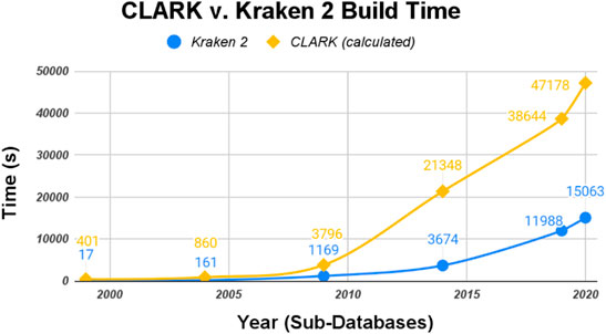
FIGURE 3. CLARK and Kraken 2 raw Build Time (seconds).

The raw data was then normalized with the size of each classifiers’ sub-databases (in gigabytes shown in Figure 4 and the number of genomes shown in Figure 5). CLARK has an unusually large build time/GB for the smallest database (1999), and then the time per GB decreases drastically. Kraken 2’s build time/GB for the 1999 database is also much larger than its build time for the other five databases, but it is still 30x shorter than CLARK’s build time for the 1999 database. Also, Kraken 2’s build time for the other five databases are less than half that of CLARK’s in time/GB and even more for time/genome. Overall, even when normalized to account for the difference in the size of databases and number of genomes, Kraken 2’s database building procedure ran several times faster than CLARK’s.

FIGURE 4

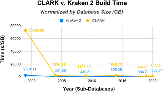
FIGURE 4. CLARK and Kraken 2 Build Time normalized by database size (seconds/Gigabyte).

FIGURE 5

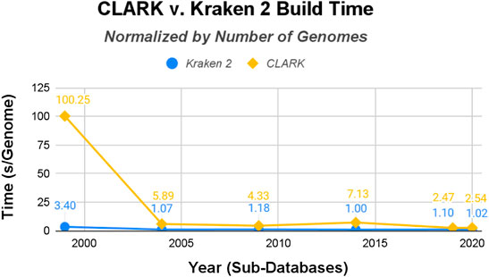
FIGURE 5. CLARK and Kraken 2 Build Time normalized by the number of genomes in the databases (seconds/genome).

Classification Time

Conversely, CLARK’s procedure is faster at classifying than Kraken 2’s. Just by raw numbers, shown in Figure 6, CLARK had the shorter classification time for the 1999, 2004, 2009, and 2014 databases. Its classification time for the 2019 and 2020 databases, however, were longer than Kraken 2’s.

FIGURE 6

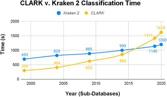
FIGURE 6. CLARK and Kraken 2 raw Classification Time (seconds).

Normalizing the raw data by gigabytes (see Figure 7) and genomes (see Figure 8), this time-trend remains similar. While both start out with particularly long runtimes for their classification procedures, Kraken 2’s is substantially higher and remains that way, even after the drastic decrease after the 1999 database. But this time their runtimes are much closer in value than the build/training times. CLARK classifies several times faster for time/GB, but they are both similar in time/genome. Overall, the methods are designed to perform the classification procedure magnitudes faster than the build time, since users usually want results quickly and are willing to spend a one-time longer cost up-front.

FIGURE 7

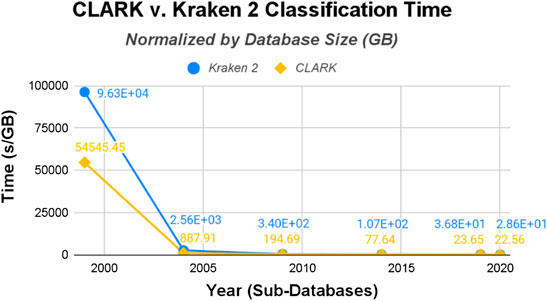
FIGURE 7. CLARK and Kraken 2 Classification Time normalized by the size of the databases (seconds/Gigabyte).

FIGURE 8

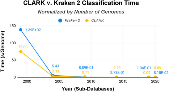
FIGURE 8. CLARK and Kraken 2 Classification Time normalized by the number of genomes in the databases (seconds/genome).

Classification Results

Since there is no ground truth classification for the gut microbiome sample, there is no way to check how accurate CLARK or Kraken 2’s classifications are, but we can examine how the number of reads classified changes as more genomes are added to their databases.

CLARK generally had a higher percentage of classified reads for all sub-databases except 2020, as shown in Figure 9. Even when Kraken 2 had more genomes in its database to reference, CLARK’s percent-classified was still higher. In 2004, CLARK classifies about 5% of sequences while Kraken 2 classifies 1% (see relative abundance tables in Supplementary Material), and this difference compounded with the limitations of the databases causes a significant dissimilarity between the classifiers (shown later in Figure 20). Also, CLARK’s percentage of classified reads dropped suddenly and drastically with the 2020 sub-database.

FIGURE 9

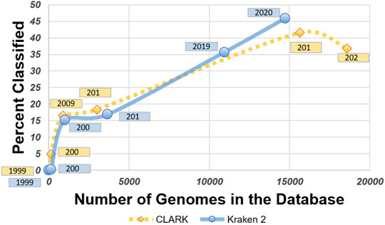
FIGURE 9. Graph comparing the number of genomes in their databases with the percent classified for each sub-database for CLARK and Kraken 2.

While Kraken 2’s classification percentages seemed to increase steadily in an exponential curve, as shown in Figure 11, CLARK’s had an unexpected decrease after 2019, as shown in Figure 10. Figures 10, 11 show that CLARK and Kraken 2 classified reads in a similar fashion for genus level, in terms of quantity and identity. Since CLARK classified more than Kraken 2 in 2004, in Figure 10, it found Bacteroides as the first genus to rise above the 3% threshold (that we used for visualization). However, for 2020, CLARK only classified about 37% of the sample while Kraken 2 classified nearly 50% (see relative abundance tables in Supplementary Material). Also, Bacteroides and Phocaeicola are the dominant genera detected by both metagenomic classifiers. By 2020, for Phocaeicola, CLARK and Kraken 2’s general relative abundance percentages were 10.66% and 13.47% respectively (see relative abundance tables in Supplementary Material). For Bacteroides, their percentages were 20.37% and 31.26% respectively (see relative abundance tables in Supplementary Material).

FIGURE 10

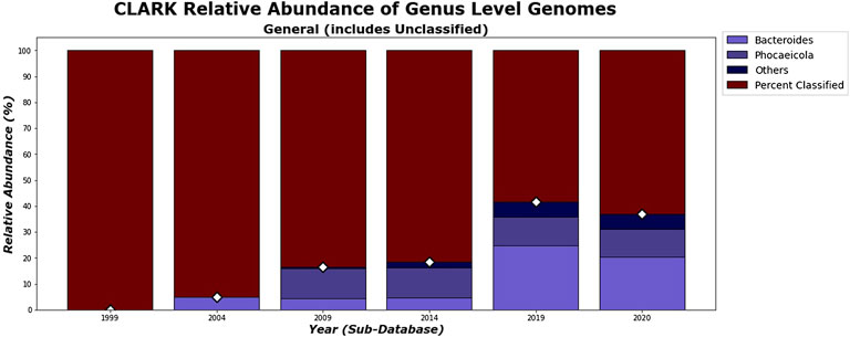
FIGURE 10. CLARK’s general relative abundance for Genus Level. Only taxa whose general relative abundance was at least 3% are shown as a colored bar here. A bar for the Unclassified group is included. The percentage of classified reads for each year are shown as diamond markers.

FIGURE 11

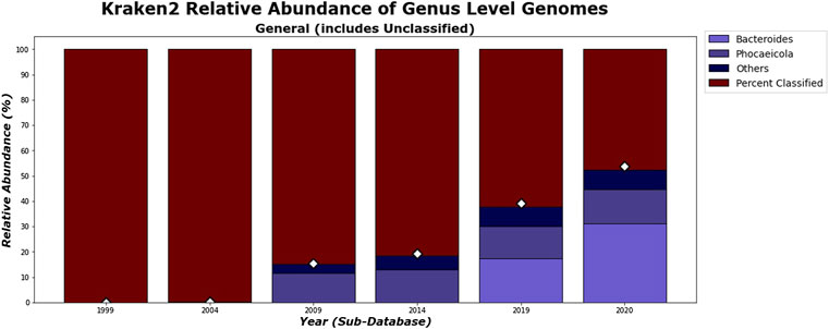
FIGURE 11. Kraken 2’s general relative abundance for Genus level. Only taxa whose general relative abundance was at least 3% are shown as a colored bar here. A bar for the unclassified group is included. The percentage of classified reads for each year are shown as diamond markers.

In Figures 12, 13, the differences between the genera that CLARK and Kraken 2 classified are shown. It is also notable to mention that CLARK and Kraken 2 did not detect Bacteroides to the same extent using the 1999 and 2004 sub-databases. This is probably due to CLARK’s ability to detect Bacteroides given the limited database. Kraken 2 did not detect as many and therefore, other bacteria genera (e.g. Bacteroidetes such as Porphyromonas) were found in high abundance. Also in 2004, neither classifier detected Phocaeicola in any significant amount, probably due to the absence of that bacteria from the database.

FIGURE 12

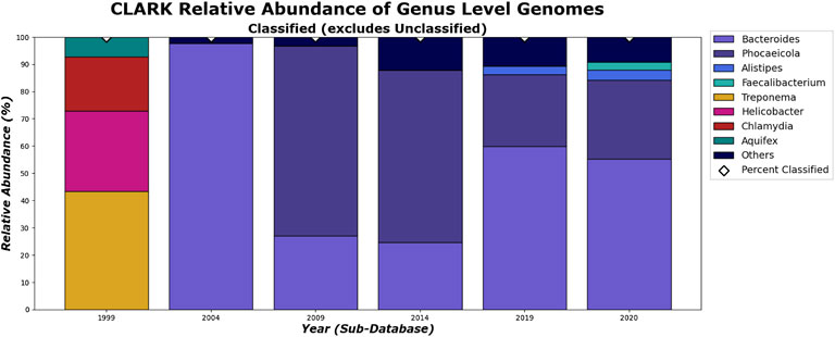
FIGURE 12. CLARK’s classified relative abundance for Genus Level. Only taxa whose classified relative abundance was at least 3% are shown as a colored bar here. Only bars for classified reads are included. The percentage of classified reads traced back to genus level for each year are shown as diamond markers.

FIGURE 13

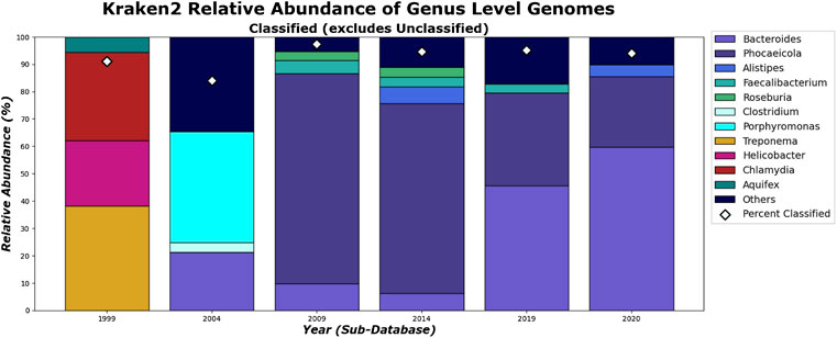
FIGURE 13. Kraken 2’s relative abundance for Genus level. Only taxa whose classified relative abundance was at least 3% are shown as a colored bar here. Only bars for the classified reads are included. The percentage of classified reads traced back to genus level for each year are shown as diamond markers.

What can be more contentious is the detection of Alistipes and Faecalibacterium. While Faecalibacterium prausnitzii is detected in the species level for 2009 and after for Kraken 2 (Figure 15), it is not detected in the genus level in 2020 (Figure 13). This is due to Kraken 2’s ability to assign more reads at the genus level than the species level and while the Faecalibacterium has the same number of reads in each, it falls below our 3% threshold for the genus level. In fact, because Kraken 2 classifies less reads, there is more of a diversity of bacteria meeting this 3% threshold as shown in Figures 13, 15. However, for the 3 most abundant genera, the classifications tend to agree more when run on recent databases.

On the species level, shown in Figures 14, 15. CLARK and Kraken 2’s classification results also differ slightly in what they classified. For example, only Bacteroides sp. M10 is found with Kraken 2, and this may be due to the different species in the different methods’ databases. However, by 2020, the methods tend to be in more agreement on the sample composition. It is also interesting to note that everything that CLARK classifies, it classifies on all levels (Figures 12, 14), while Kraken 2 has different percentages classified on each taxonomic level (Figures 13, 15.)

FIGURE 14

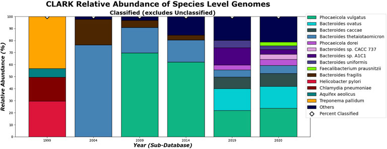
FIGURE 14. CLARK’s relative abundance for Species level. Only taxa whose classified relative abundance was at least 3% are shown as a colored bar here. Only bars for classified reads are included. The percentage of classified reads traced back to species level for each year are shown as diamond markers.

FIGURE 15

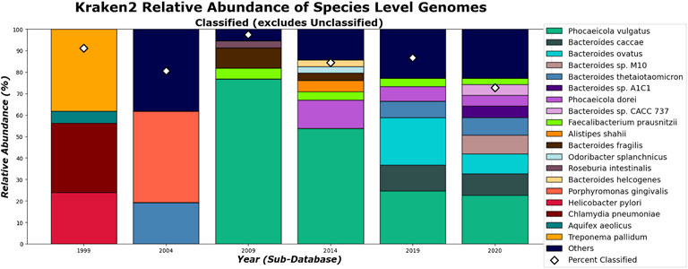
FIGURE 15. Kraken 2’s relative abundance for Species level. Only taxa whose classified relative abundance was at least 3% are shown as a colored bar here. Only bars for the classified reads are included. The percentage of classified reads traced back to species level for each year are shown as diamond markers.

We can see how increasing knowledge added to the training database changes the classification results over time–using the Bray-Curtis dissimilarity measure from the ecological literature to quantify ecosystem dissimilarity. As expected, the Bray-Curtis dissimilarity shows that the classification results of the gut microbiome sample generally become less similar as the time increases between sub-database versions, shown in Figures 16–19. An exception is the Bray-Curtis dissimilarity between the 2009 and 2014 sub-databases of both CLARK and Kraken 2. That dissimilarity is even lower than the dissimilarity between the 2019 and 2020 sub-databases (see Bray-Curtis dissimilarity tables in Supplementary Material).

FIGURE 16

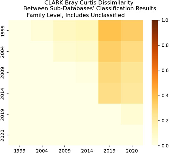
FIGURE 16. CLARK’s Bray-Curtis dissimilarity score for Family level. It is a comparison between each sub-databases’ classification results for CLARK. It includes comparisons of what CLARK classified as well as what CLARK didn’t classify for each year. It is interesting that 2009–2014 databases yield the most similar results on the family level (more similar than 2019–2020).

FIGURE 17

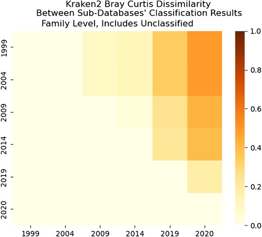
FIGURE 17. Kraken 2’s Bray-Curtis dissimilarity score for Family level. It is a comparison between each sub-databases’ classification results for Kraken 2. It includes comparisons of what Kraken 2 classified as well as what it didn’t classify for each year. Unlike CLARK, Kraken 2’s most similar results are from the 1999 and 2004 databases.

FIGURE 18

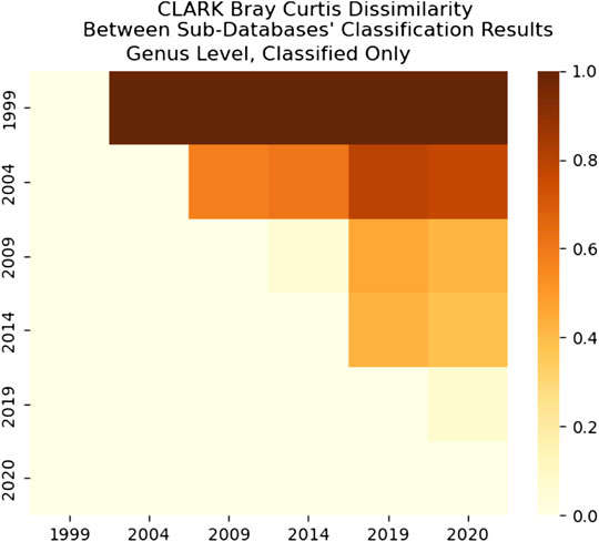
FIGURE 18. CLARK’s Bray-Curtis Dissimilarity score for Genus level. It is a comparison between each sub-databases’ classification results. It only includes what CLARK classified. It is interesting that 1999 results are significantly different from any other years’, while 2009–2014 and 2019–2020 are the most similar.

FIGURE 19

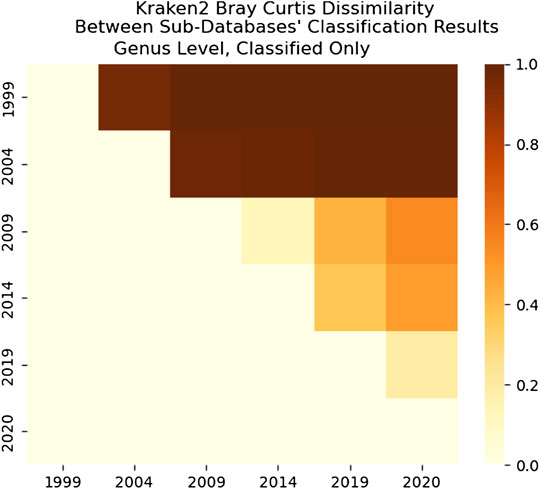
FIGURE 19. Kraken 2’s Bray-Curtis Dissimilarity score for Genus level between each sub-databases’ classification results. The comparison shows that classified results are more similar for successive databases–although some are more similar than others (such as 1999–2004 and 2009–2014).

As we can see in Figure 18, the dissimilarity is greatest between the CLARK classifications on the genus level between 1999 and any other year, since only a handful of genera were known and CLARK had a large number of percent classified in 2004 (seen in Figures 10, 12, 14) compared to Kraken 2. For Kraken 2, since the percent classified did not increase for 2004, the 1999 and 2004 classification results are very similar, as seen in Figures 17, 19. This is also true for 2009 to 2014 for genus and family level classifications for both CLARK nor Kraken 2 (and result in more similar results than the transition from 2019 to 2020), as seen in Figures 16–19. This similarity reflects how the change in percent classified (for both CLARK and Kraken 2) between the 2009 to 2014 database years was the smallest change seen in all the years (seen in Figures 10–15). This can be due to the fact that the database additions did not add the gut microbes that they are in or relatives of those in this metagenomic sample, and those additions came later.

Finally, in Figure 20, we show the Bray-Curtis dissimilarity between CLARK and Kraken 2 for each year and taxonomic level. Interestingly, both make the same classifications in 1999 and are pretty similar. In 2004, the dissimilarity is mainly because CLARK classifies many more percentages of sequences than Kraken 2 (which the Bray-Curtis measure takes into consideration). CLARK classifying more sequences makes the methods more discordant at higher levels of taxonomic tree in 2009. Since the family level has many more classes than order, class, phyla, the Bray-Curtis values are very high for cases where taxa exists in one classifier but not the other, and this is much less likely with less classes at higher taxonomic levels. Taxa that are uniquely classified by each method also contribute to dissimilarity, but they are not the main contributors to the large dissimilarity value. Interestingly, after 2004, in time, both methods then become more concordant with increasing knowledge, with some deviation in species and more concordance on the phylum level. Now, in the latest 2020 database update, the results are slightly more discordant than in 2009, despite having many more taxa classes, showing that the methods are able to agree when the relevant gut taxa that is “truly” in the sample is added to the database.

FIGURE 20

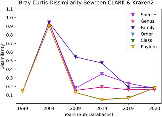
FIGURE 20. The Bray-Curtis dissimilarity between the classified results of CLARK and Kraken 2 for each taxonomic level over time (increasing database size). Since only 4 organisms from 4 different phyla were classified in 1999, the similarity of the results is close. In 2004, a distinct issue is that CLARK classified significantly more reads than Kraken 2, which skewed the dissimilarity to be significant for all taxonomic levels. In 2009, the methods are more concordant, and for the rest of the years, the species-level classification is different while the phylum classification is more similar. The methods are pretty similar on all taxonomic levels once again in 2020.

Discussion

CLARK’s method of only comparing unique k-mers from a read to its target genomes may have been what aided its classification time but hindered its classification percentage. Because CLARK ignores any k-mer in a read that is shared between two or more targets (genomes in its database), it can work through data more quickly. This method seems to allow it to eliminate unlikely matches more efficiently. However, this also seems to make it harder to match k-mers uniquely to genomes that are closely related (ie. species level). The elimination of targets that have one of the read’s k-mers in common could cause CLARK to eliminate many genomes from being possible matches, most likely ending up with no more targets to compare and resulting in an unclassified read. This could explain why CLARK’s classification percentage decreased between the 2019 and 2020 databases so drastically: as more and more similar species were added, it became harder and harder for CLARK to match unique k-mers to them.

Despite CLARK having more genomes in its database to get through, it still classified faster than Kraken 2 under normalized circumstances. This could be due to how it decides which genome best matches the read. CLARK may be classifying faster because it only has to keep track of the unique k-mers in a read and compare its targets to those, while ignoring the common k-mers. While Kraken 2 has to keep track of all the common k-mers for every genome it is comparing.

In the future, a further study should be conducted with carefully designed mock communities or simulated communities with CAMISIM (Fritz et al., 2019) to make sure a carefully balanced novel/known set is contained in the training/test sets. However, much is still not known about the underlying k-mer distribution of novel organisms and their frequency.

Conclusion

In this paper, we compose a framework in which to compare metagenomic taxonomic classifiers, in terms of their computational time and classification agreement on a real metagenomic sample. We studied hash-based methods and found that a technique that eliminates common k-mers, CLARK, classifies more and faster (at a cost of longer training time) when trained on smaller and more diverse databases. However, the percent of the sample that it can classify starts to degrade for large databases. Kraken 2, on the other hand, gains percent classified and significantly takes less time building and classifying with more training data. Both methods’ agreement on classification labels tend to converge as the database knowledge in each grows, and the database differences can cause some divergence between the two methods’ classifications. The recommendation from our study is that Kraken 2 tends to scale better with more data. However, we recommend for future studies to extend this study and compare many methods’ scalability in terms of time, percent classified, and agreement with the experimental framework that we introduce here.

Data Availability Statement

The original contributions presented in the study are included in the article/Supplementary Material, further inquiries can be directed to the corresponding author.

Author Contributions

MG wrote the original draft, assisted in conceptualization, and implemented all the methodology, analysis, validation, and visualization. ZZ organized and curated the data(bases) and assisted in methodology, analysis, validation, and visualization. GR conceptualized the study, acquired funding, supervised and coordinated the project, assisted with the methodology with analysis, methodology, and visualization and assisted in writing the original draft.

Funding

This work was supported by NSF grants #1919691, #1936791, and #2107108 that supported students and computer infrastructure needed for the project.

Conflict of Interest

The authors declare that the research was conducted in the absence of any commercial or financial relationships that could be construed as a potential conflict of interest.

Publisher’s Note

All claims expressed in this article are solely those of the authors and do not necessarily represent those of their affiliated organizations, or those of the publisher, the editors and the reviewers. Any product that may be evaluated in this article, or claim that may be made by its manufacturer, is not guaranteed or endorsed by the publisher.

Supplementary Material

The Supplementary Material for this article can be found online at: https://www.frontiersin.org/articles/10.3389/frsip.2022.842513/full#supplementary-material

References

Alshawaqfeh, M. K. (2017). Signal Processing and Machine Learning Techniques for Analyzing Metagenomic Data. Thesis. College Station, TX: Texas A&M. Available at: https://oaktrust.library.tamu.edu/handle/1969.1/161461.

Google Scholar

Berg, G., Rybakova, D., Fischer, D., Cernava, T., Vergès, M.-C., Charles, T., et al. (2020). Microbiome Definition Re-Visited: Old Concepts and New Challenges. Microbiome 8 (1), 103. doi:10.1186/s40168-020-00875-0

PubMed Abstract | CrossRef Full Text | Google Scholar

Borrayo, E., Mendizabal-Ruiz, E. G., Vélez-Pérez, H., Romo-Vázquez, R., Mendizabal, A. P., and Morales, J. A. (2014). Genomic Signal Processing Methods for Computation of Alignment-Free Distances from DNA Sequences. PLOS ONE 9 (11), e110954. doi:10.1371/journal.pone.0110954

PubMed Abstract | CrossRef Full Text | Google Scholar

Brown, T., and Irber, L. (2016). Sourmash: A Library For Minhash Sketching of DNA. J. Open Source Softw. 1 (5), 27. doi:10.21105/joss.00027

CrossRef Full Text | Google Scholar

Brul, S., Kallemeijn, W., and Smits, G. (2010). Functional Genomics for Food Microbiology: Molecular Mechanisms of Weak Organic Acid Preservative Adaptation in Yeast. CAB Rev.: Perspect. Agric. Vet. Sci. Nutrit. Nat. Resources 3 (January), 1–14. doi:10.1079/PAVSNNR20083005

CrossRef Full Text | Google Scholar

Coenen, A. R., Hu, S. K., Luo, E., Muratore, D., and Weitz, J. S. (2020). A Primer for Microbiome Time-Series Analysis. Front. Genet. 11, 310. doi:10.3389/fgene.2020.00310

PubMed Abstract | CrossRef Full Text | Google Scholar

Creasy, H. H., Felix, V., Aluvathingal, J., Crabtree, J., Ifeonu, O., Matsumura, J., et al. (2021). HMPDACC: A Human Microbiome Project Multi-Omic Data Resource. Nucleic Acids Res. 49 (D1), D734–D742. doi:10.1093/nar/gkaa996

PubMed Abstract | CrossRef Full Text | Google Scholar

dibsi-rnaseq (2016). Sourmash Website. Available at: https://dibsi-rnaseq.readthedocs.io/en/latest/kmersand-sourmash.html (Accessed May 16, 2022).

Google Scholar

Elworth, R. A. L., Wang, Q., KotaKota, P. K., Barberan, C. J., Coleman, B., Balaji, A., et al. (2020). To Petabytes and Beyond: Recent Advances in Probabilistic and Signal Processing Algorithms and Their Application to Metagenomics. Nucleic Acids Res. 48 (10), 5217–5234. doi:10.1093/nar/gkaa265

PubMed Abstract | CrossRef Full Text | Google Scholar

Figueiredo, A. R. T., and Kramer, J. (2020). Cooperation and Conflict within the Microbiota and Their Effects on Animal Hosts. Front. Ecol. Evol. 8, 132. doi:10.3389/fevo.2020.00132

CrossRef Full Text | Google Scholar

Fritz, A., Hofmann, P., Majda, S., Dahms, E., Dröge, J., Fiedler, J., et al. (2019). CAMISIM: Simulating Metagenomes and Microbial Communities. Microbiome 7, 17. doi:10.1186/s40168-019-0633-6

PubMed Abstract | CrossRef Full Text | Google Scholar

Garbarine, E., DePasquale, J., Gadia, V., Polikar, R., and Rosen, G. (2011). Information-Theoretic Approaches to SVM Feature Selection for Metagenome Read Classification. Comput. Biol. Chem. 35 (3), 199–209. doi:10.1016/j.compbiolchem.2011.04.007

PubMed Abstract | CrossRef Full Text | Google Scholar

Gardner, P. P., Watson, R. J., Draper, J. L., Finn, R. D., Morales, S. E., and Stott, M. B. (2019). Identifying Accurate Metagenome and Amplicon Software via a Meta-Analysis of Sequence to Taxonomy Benchmarking Studies. PeerJ 7, e6160. doi:10.7717/peerj.6160

PubMed Abstract | CrossRef Full Text | Google Scholar

Huttenhower, C., Gevers, D., Knight, R., Abubucker, S., Badger, J. H., Chinwalla, A. T., et al. (2012). Structure, Function and Diversity of the Healthy Human Microbiome. Nature 486 (7402), 207–214. doi:10.1038/nature11234

PubMed Abstract | CrossRef Full Text | Google Scholar

Kouchaki, S., Tapinos, A., and Robertson, D. L. (2019). A Signal Processing Method for Alignment-Free Metagenomic Binning: Multi-Resolution Genomic Binary Patterns. Sci. Rep. 9 (1), 2159. doi:10.1038/s41598-018-38197-9

PubMed Abstract | CrossRef Full Text | Google Scholar

Lan, Y., Morrison, J. C., Hershberg, R., and Rosen, G. L. (2014). POGO-DB-a Database of Pairwise-Comparisons of Genomes and Conserved Orthologous Genes. Nucl. Acids Res. 42 (D1), D625–D632. doi:10.1093/nar/gkt1094

PubMed Abstract | CrossRef Full Text | Google Scholar

LaPierre, N., Alser, M., Eskin, E., Koslicki, D., and Mangul, S. (2020). Metalign: Efficient Alignment-Based Metagenomic Profiling via Containment Min Hash. Genome Biol. 21, 242. doi:10.1186/s13059-020-02159-0

PubMed Abstract | CrossRef Full Text | Google Scholar

Liu, S., and Koslicki, D. (2021). CMash: Fast, Multi-Resolution Estimation of K-Mer-Based Jaccard and Containment Indices. BioRxiv. doi:10.1101/2021.12.06.47143

CrossRef Full Text | Google Scholar

McIntyre, A. B. R., Ounit, R., Afshinnekoo, E., Prill, R. J., Hénaff, E., Alexander, N., et al. (2017). Comprehensive Benchmarking and Ensemble Approaches for Metagenomic Classifiers. Genome Biol. 18, 182. doi:10.1186/s13059-017-1299-7

PubMed Abstract | CrossRef Full Text | Google Scholar

Meyer, F., Fritz, A., Deng, Z.-L., Koslicki, D., Gurevich, A., Robertson, G., et al. (2021). Critical Assessment of Metagenome Interpretation - The Second Round of Challenges. Biorxiv. Available at: https://www.biorxiv.org/content/10.1101/2021.07.12.451567v1.

Google Scholar

Nasko, D. J., Koren, S., Phillippy, A. M., and Treangen, T. J. (2018). RefSeq Database Growth Influences the Accuracy of K-Mer-Based Lowest Common Ancestor Species Identification. Genome Biol. 19, 165. doi:10.1186/s13059-018-1554-6

PubMed Abstract | CrossRef Full Text | Google Scholar

Nemergut, D. R., Schmidt, S. K., Fukami, T., O'Neill, S. P., Bilinski, T. M., Stanish, L. F., et al. (2013). Patterns and Processes of Microbial Community Assembly. Microbiol. Mol. Biol. Rev. 77 (3), 342–356. doi:10.1128/MMBR.00051-12

PubMed Abstract | CrossRef Full Text | Google Scholar

Ounit, R., Wanamaker, S., Close, T. J., and Lonardi, S. (2015). CLARK: Fast and Accurate Classification of Metagenomic and Genomic Sequences Using Discriminative K-Mers. BMC Genomics 16 (1), 236. doi:10.1186/s12864-015-1419-2

PubMed Abstract | CrossRef Full Text | Google Scholar

Rosen, G. L., and Moore, J. D. (2003). “Investigation of Coding Structure in DNA,” in IEEE International Conference on Acoustics, Speech, and Signal Processing (ICASSP), Hong Kong.

Google Scholar

Rosen, G., Sokhansanj, B., Polikar, R., Bruns, M., Russell, J., Garbarine, E., et al. (2009). Signal Processing for Metagenomics: Extracting Information from the Soup. Curr. Genomics 10 (7), 493–510. doi:10.2174/138920209789208255

PubMed Abstract | CrossRef Full Text | Google Scholar

Sayers, E. W., Agarwala, R., Bolton, E. E., Brister, J. R., Canese, K., Clark, K., et al. (2019). Database Resources of the National Center for Biotechnology Information. Nucleic Acids Res. 47 (D1), D23–D28. doi:10.1093/nar/gky1069

PubMed Abstract | CrossRef Full Text | Google Scholar

Scipy (2021). Scipy.Spatial.Distance.Braycurtis — SciPy v1.7.1 Manual. Available at: https://docs.scipy.org/doc/scipy/reference/generated/scipy.spatial.distance.braycurtis.html (Accessed December 1, 2021).

Google Scholar

Sczyrba, A., Hofmann, P., Belmann, P., Koslicki, D., Janssen, S., Dröge, J., et al. (2017). Critical Assessment of Metagenome Interpretation-A Benchmark of Metagenomics Software. Nat. Methods 14, 1063–1071. doi:10.1038/nmeth.4458

PubMed Abstract | CrossRef Full Text | Google Scholar

Sender, R., Fuchs, S., and Milo, R. (2016). Are We Really Vastly Outnumbered? Revisiting the Ratio of Bacterial to Host Cells in Humans. Cell 164 (3), 337–340. doi:10.1016/j.cell.2016.01.013

PubMed Abstract | CrossRef Full Text | Google Scholar

Shi, L., and Chen, B. (2021). “LSHvec: A Vector Representation of DNA Sequences Using Locality Sensitive Hashing and Fasttext Word Embeddings,” in Proceedings of the 12th ACM Conference on Bioinformatics, Computational Biology, and Health Informatics (BCB '21), New York, NY, USA, August 1–4, 2021 (Association for Computing Machinery). doi:10.1145/3459930.3469521

CrossRef Full Text | Google Scholar

Woloszynek, S., Pastor, S., Mell, J. C., Nandi, N., Sokhansanj, B., Rosen, G. L., et al. (2016). “Engineering Human Microbiota: Influencing Cellular and Community Dynamics for Therapeutic Applications,” in International Review Of Cell And Molecular Biology (Cambridge, MA: Academic Press), 324, 67–124. doi:10.1016/bs.ircmb.2016.01.003

PubMed Abstract | CrossRef Full Text | Google Scholar

Woloszynek, S., Zhao, Z., Chen, J., Gail, L., Woloszynek, S., Zhao, Z., et al. (2019). 16S rRNA Sequence Embeddings: Meaningful Numeric Feature Representations of Nucleotide Sequences that Are Convenient for Downstream Analyses. PLoS Comput. Biol. 15 (2), e1006721. doi:10.1371/journal.pcbi.1006721

PubMed Abstract | CrossRef Full Text | Google Scholar

Wood, D. E., and Salzberg, S. L. (2014). Kraken: Ultrafast Metagenomic Sequence Classification Using Exact Alignments. Genome Biol. 15 (3), R46. doi:10.1186/gb-2014-15-3-r46

PubMed Abstract | CrossRef Full Text | Google Scholar

Wood, D. E., Lu, J., Ben, L., Wood, D. E., Lu, J., and Langmead, B. (2019). Improved Metagenomic Analysis with Kraken 2. Genome Biol. 20 (1), 257. doi:10.1186/s13059-019-1891-0

PubMed Abstract | CrossRef Full Text | Google Scholar

Ye, S. H., Siddle, K. J., Park, D. J., and Sabeti, P. C. (2019). Benchmarking Metagenomics Tools for Taxonomic Classification. Cell. 178 (4), 779–794. doi:10.1016/j.cell.2019.07.010

PubMed Abstract | CrossRef Full Text | Google Scholar

Zhao, Z., Cristian, A., Rosen, G., Zhao, Z., Cristian, A., and Rosen, G. (2020). Keeping Up with the Genomes: Efficient Learning of Our Increasing Knowledge of the Tree of Life. BMC Bioinforma. 21, 412. doi:10.1186/s12859-020-03744-7

PubMed Abstract | CrossRef Full Text | Google Scholar