Learning Resource Allocation in Active-Passive Radar Sensor Networks

Recent advances in Passive Coherent Location (PCL) systems make combined active and passive radar sensor networks very attractive for both military and civilian air surveillance. PCL systems seem promising as cost-effective gap fillers of active radar coverage especially in alpine terrain and also as covert early warning sensors. However, PCL systems are sensitive to changes of Transmitters of Opportunity (ToO). Many approaches for energy-efficient target detection have been proposed for active radar sensor networks. However, energy-efficiency and topology optimization of combined active-passive radar sensor networks in realistic scenarios have been poorly studied until today. We here propose an unsupervised learning approach for topology optimization and energy-efficient detection in combined active-passive radar sensor networks. The interdependence of active and passive sensors in the network and the given target scenario is naturally accounted for by our approach. Optimal power budget and detection sectors of active radars and the most useful ToOs for each PCL sensor are simultaneously learned over time. This is a critical contribution for minimizing the need for active radar power budget and PCL computational resources. The power budget of active radars is minimized in a way that the added value of PCL sensors is fully exploited. We also demonstrate how our approach dynamically relearns to achieve robust performance when changes in the ToO of PCL sensors occur. We test our approach in a simulation suite for active-passive radar sensor networks using real-world air surveillance data and ToOs under real-world topographical conditions.

1 Introduction

Conventional Radar Sensor Networks (RSN) consist of multiple active radars (referred to as nodes) used to transmit waveforms in order to detect and track air targets. The goal of an RSN is to maximize surveillance coverage and minimize both interference between single nodes and the total power consumption of the RSN (Baker and Trimmer, 2000) (Baker and Hume, 2003). In our case we intend to minimize the usage of active radars by maximizing the usage of passive radar in the RSN, which is preferable for covert operation scenarios ¹. Widely used approaches to attack this problem include game-theoretic approaches (Bacci et al., 2012) and network cost based strategies (Jiang et al., 2019). Although such approaches are highly effective for RSNs consisting of solely active radar sensors, the widely awaited integration of Passive Coherent Location (PCL) systems pose challenges that still need to be addressed.

PCL systems have enjoyed wide interest in recent years in both research and industry. Commercial systems are currently at the verge of operational go-live for diverse defense and civilian surveillance purposes. PCL systems are attractive due to their cost-effectiveness and covert operational capability. However, efficient deployment of passive radar is relatively complex due to their dependence on the so called Transmitters-of-Opportunity (ToO). Especially in alpine terrain, the operation of a PCL system can be crucially affected by topographical conditions and ToO properties. In the alpine terrain many ToOs exhibit highly directional transmission gains in order to optimize transmission patterns owing to topological and urban requirements. Transmission power and vertical/horizontal antenna transmission constraints of the ToOs make pre-deployment mission planning of PCL systems and especially optimization of receiver locations (Mathews et al., 2015) (Mousel, 2017) or ToO selection for fixed receiver sites computationally challenging. Moreover, the number of usable ToOs per PCL sensor is restricted by the limited computational resources available at the sensor site and the receiver bandwidth, making it inevitable to determine the most useful ToOs for each PCL sensor. Currently available PCL systems mainly use heuristics, on site signal measurements and human expertise to solve the above issues.

Consequently, the efficient integration of PCL systems into an existing active radar only RSN system, although topic of ongoing research, poses several operational and logistics of deployment challenges. These challenges have not yet been addressed neither by game theory nor by radar research communities. We here propose a simulation based approach for online learning of useful ToOs per PCL sensor and optimal power budget and detector sector of active sensors. Online refers to the fact that our approach if deployed in a running sensor network will learn the efficient deployment topology and active radar emission control over time with the goal of finding the optimal ToOs for each PCL sensor and the most useful range-sector bins for each active radar sensor. The proposed methodology goes beyond the conventional radar coverage computations for given altitudes and proposes a temporal online learning mechanism. Our simulation suite uses models of passive and active radar detection, topography, wave propagation and real-world ToOs in continental Europe. Our approach proposes to use Hebbian learning to efficiently determine the most useful ToOs per PCL sensor to maximize the PCL system’s added value for coverage in an active-passive RSN. At the same time the proposed neural network also learns the optimal active radar power budget and sectors. We feed the simulation with real-world recorded air surveillance data to adapt the Hebbian plasticity of the used neural network. In summary our approach proposes an efficient online learning mechanism to compute the optimal spatiotemporal coverage of a combined active-passive sensor network.

2 Research Question

Conventionally, comparison of static coverage diagrams of PCL systems with those of active radars are used to manually perform mission and deployment planning. This very often leads to locally or partially optimal solutions that cannot be easily scaled or adapted to new scenarios. With the upcoming integration of PCL systems into operational civil and military sensor networks, the need for topological and power budget optimization of such multiband active-passive systems is given. In the current work we propose a simulation based methodology to learn the efficient deployment of each node in an active-passive radar network. Our approach was motivated by the high transmission constraints of ToOs and severe topological challenges in alpine terrain.

Given a set of active radars and PCL sensors on certain locations, we address the problem of simultaneously determining the most useful ToOs for each PCL sensor and the most effective power budget strategy for each active radar. With “useful” ToOs we mean the ToOs that provide more detections compared to others. Such useful ToOs per PCL sensor can differ depending on the target scenario and the available set of active radars and other PCL sensors. Similarly, the optimal power budget (consisting of the most useful range-sector bins) for each active radar in the sensor network depends on the target scenario and the available PCL sensors and active radars. We here investigate the target scenario over continental Europe around Switzerland on a normal day. The daily air traffic over continental Europe is to a very high extent constant during periods of no tension. Given this real-world target scenario and a set of PCL and active radar sensors with their locations in Switzerland, we address the problem of finding the most useful ToOs per PCL sensor (from the hundreds of real-world ToOs available) and the most useful range-sector bins for active radars. Our goal is to simultaneously minimize the emissions of active radars or even to totally eliminate their usage and determine the most useful PCL ToOs. Instead of conventional game theoretic approaches with relatively simplistic sensor nodes and probabilistic target detection models we propose a Hebbian learning method using models of sensors, topography, targets and wave propagation for coverage predictions of active and passive radar systems for a replayed real-world air traffic scenario.

3 Active and Passive Sensor Models

In this section, we discuss the PCL and active radar detection models used in our RSN simulation suite.

3.1 Passive Coherent Location Sensor

We assume that the transmitters and receivers are given with the following parameters respectively:

3.1.1 Bistatic Doppler Shift Computation

We consider a moving target and stationary transmitters and receivers. A canonical definition of bistatic Doppler shift f_D, ignoring relativistic effects, is the rate of change of the total path length of the transmitted signal, normalized by the wavelength λ (Jackson, 1986). The total path length is the range sum $\Vert \overrightarrow{R_T}\Vert +\Vert \overrightarrow{R_R}\Vert$.

The bistatic Doppler shift can be written using the derivatives of the range sum as:

$f_D=\frac{1}{\lambda }\left[\frac{d\Vert \overrightarrow{R_T}\Vert }{dt}+\frac{d\Vert \overrightarrow{R_R}\Vert }{dt}\right](1)$

The target’s velocity vector projected onto the bistatic plane (defined by the vectors $\overrightarrow{R_T}$ and $\overrightarrow{R_R}$) has the magnitude v and aspect angle δ referenced to the bistatic bisector (the aspect angle is positive when measured clockwise from the bistatic bisector). Figure 1 for an illustration.

FIGURE 1

FIGURE 1. Geometry visualization for bistatic Doppler computation (λ is the signal wavelength).

The term $d\Vert \overrightarrow{R_T}\Vert /dt$ is the projection of the target velocity vector onto the transmitter-to-target LoS:

$\frac{d\Vert \overrightarrow{R_T}\Vert }{dt}=v\cdot \mathit{cos}\left(\delta -\beta /2\right)(2)$

Similarly, $d\Vert \overrightarrow{R_R}\Vert /dt$ is the projection of the target velocity vector onto the receiver-to-target LoS:

$\frac{d\Vert \overrightarrow{R_R}\Vert }{dt}=v\cdot \mathit{cos}\left(\delta +\beta /2\right)(3)$

Combining Equations 1 and 2 and 3 we write the bistatic Doppler shift caused by target motion as:

$\begin{array}{ccc}\hfill f_D=\frac{v}{\lambda }\left[\mathit{cos}\left(\delta -\beta /2\right)+\mathit{cos}\left(\delta +\beta /2\right)\right]& \hfill & \hfill \end{array}(4)$

$\begin{array}{ccc}\hfill =\frac{2v}{\lambda }\mathit{cos}\left(\delta \right)\mathit{cos}\left(\frac{\beta }{2}\right)& \hfill & \hfill \end{array}(5)$

Target detection using a simulated PCL sensor is reported when a bistatic Doppler threshold is surpassed. This means that bistatic geometry for PCL detection is taken into account in our simulation. Besides bistatic Doppler, also the Signal-to-Noise Ratio (SNR) is computed and thresholded. The specific threshold values for both bistatic Doppler and SNR are discussed below in section 3.1.2.

3.1.2 PCL Detection Model

We use the well known bistatic radar Equation to compute the Signal-to-Noise Ratio (SNR):

$SNR=\frac{P_r}{P_n}=\frac{P_t{G}_t}{4\pi r_1^2}{\sigma }_b\frac{1}{4\pi r_2^2}\frac{G_r{\lambda }^2}{4\pi }\frac{G_p}{k{T}_{0}BF}L(6)$

where we define the following:

We compute processing gain G_p as B*t_int where B is receiver bandwidth and t_int is integration time. Further, we set a detection threshold of 5 Hz Doppler shift and 14 dB SNR.

For illustrating the passive radar coverage we use the notion of minimum detectable RCS. Instead of solving for an achievable SNR we calculate the minimal needed RCS σ_B, min that is required for detection. For this we rewrite the SNR Eq. (6) such that it is independent of the bistatic RCS σ_B:

$SN{R}_{{\sigma }_B}=\frac{SNR}{{\sigma }_B}(7)$

Now by requiring that the SNR of a target to be greater than a threshold SNR_thr we derive an expression giving a lower bound for the RCS of the target:

${\sigma }_B>\frac{SN{R}_{thr}}{SN{R}_{{\sigma }_B}}={\sigma }_{B,\mathit{min}}(8)$

Expressing SNR in dB yields Eq. (8) as:

${\sigma }_B>10^{\left(SN{R}_{thr,dB}-SN{R}_{{\sigma }_B,dB}\right)/10}={\sigma }_{B,\mathit{min}}(9)$

In order to be detectable, a target needs to have an RCS greater than the minimum RCS required for detection, σ_B, min. This allows plotting passive radar coverage as minimum detectable RCS as shown in section 7.

A complete discussion of performance prediction using the bistatic radar Equation can be found in (Griffiths and Baker, 2005). A simulation of passive Radar detection performance prediction using antenna patterns and propagation effects is performed and compared with real world measurements in Malanowski et al. (2022). An approach for optimization of passive radar receiver location was proposed in Mathews et al. (2015) and a combinatorial optimization model for the joint placement of transmitters and receivers was proposed in Yi et al. (2017).

3.2 Active Radar Model

We assume the following parameters for a given active radar:

We consider non fluctuating targets (Swerling V model) and noise modelled as a Gaussian. Although the Swerling V is used here it is not a limiting factor for the proposed method. Given this and if the intermediate filter (IF) and the detector can be modelled as a narrow band filter, then the probability density function (PDF) of the post-detection envelope of the noise voltage can be modelled as the Rayleigh function (Barton, 2013):

$p\left(R\right)=\frac{R}{{\mathrm{\Psi }}_0}\mathit{exp}\left(\frac{-R^2}{2{\mathrm{\Psi }}_0}\right)(10)$

where R is the amplitude of the envelope of the output filter and Ψ₀ is the variance of the noise voltage. This has the form of the Rayleigh probability density function.

Given the above noise model and for a given constant false alarm rate (typically $<10^{-6}$) we now consider the probability of detection pd. A sine wave with amplitude A and frequency f₀ is considered as the signal. This signal is present along with the noise at the input to the IF filter. The frequency of the sine wave is equal to the centre frequency of the IF filter f₀ then the output of the envelope detector will have the Rician distribution as the PDF (Barton, 2013):

$p_s\left(R\right)=\frac{R}{{\mathrm{\Psi }}_0}\mathit{exp}\left(-\frac{R^2+A^2}{2{\mathrm{\Psi }}_0}\right)I_0\left(\frac{RA}{{\mathrm{\Psi }}_0}\right)(11)$

Given the Rayleigh distributed noise as in Equation 10 and a specific Signal-to-Noise Ratio (SNR), the Rician distribution for the output of the envelope detector as in Eq. (11) is defined. We define the detection threshold so that a false alarm occurs whenever the noise voltage exceeds a defined threshold voltage Vt. Now the probability of detection can be expressed as:

$p_d={\int }_{V_t}^{\infty }\frac{R}{{\mathrm{\Psi }}_0}\mathit{exp}\left(-\frac{R^2+A^2}{2{\mathrm{\Psi }}_0}\right)I_0\left(\frac{RA}{{\mathrm{\Psi }}_0}\right)dR(12)$

The above Equation can numerically be solved using Marcum’s Q-function. We use the Matlab implementation provided in (Schreiner, 1999) for computing the p_d given the above noise model, a constant false alarm rate and an SNR. Thereby the SNR of a non fluctuating target was computed using the well known radar Equation (Skolnik, 1980; Barton, 2013):

$SNR=\frac{P{T}_d{G}_t{G}_r{\lambda }^2\sigma }{{\left(4\pi \right)}^3{R}^{4}k{T}_{0}F{L}_s}(13)$

where P is average power, T_d is dwell time (= n_p*PRI), n_p is number of pulses for coherent processing, PRI is pulse repetition interval, R is radar to target distance and all other parameters the same as in section 3.1.2. We assume a fixed target RCS (σ = 10 m²). A threshold was used corresponding to the detection probability of pd > 0.8. Doppler shift is computed and thresholded analogously as for PCL in section 3.1.1. For illustrating active radar coverage computations (as in section 7) we only use the p_d threshold of 0.8, which is another way of plotting radar coverage than the minimum detectable RCS illustration discussed in section 3.1.2 for passive radar.

3.3 Radar Systems Network (RSN)

As result of the advances in PCL technology in the recent years, many nations are considering the integration of PCL systems into the existing active radar networks. PCL systems are supposed to fulfill one or many requirements such as filling the gaps in active radar coverage (gap-filling), covert surveillance and early warning. However, efficient integration of PCL systems are largely not studied yet. Our current work proposes a methodology to optimize the efficiency of both PCL and active radar systems in such an RSN.

4 Target Model

For our purposes we use non fluctuating targets with a constant RCS of 10 m² for active and passive radar on-the-fly detection simulation. Our simulation tool BURST is capable of replaying recorded air pictures consisting of hundreds of targets for several hours. Solely ADS-B recordings were used for the current work. Alternatively, more complete sources of air picture recordings such as military surveillance systems can also be used. BURST allows the configuration of the replay speed depending on the available computational resources. In the simulation testbed used for this work we could achieve four times the real recording speed, i.e. the replayed targets flew four times the speed as was originally recorded. This means that also the active and passive radar processing were performed at four times the simulated sensors real processing speed (e.g. active radar rotation time 1 s was used instead of 4 s). The maximum replay speed is limited by the available computing resources and the number of active and passive sensors to be simulated in the proportionally correct processing times as in the real world. In the case of our used computed architecture and the target/sensor scenario a speed-up of factor four was seen to be the maximum.

5 Simulation Based Optimization

5.1 Simulation Architecture

We use the homegrown simulation suite named BURST to simulate all the necessary modules. BURST is a set of loosely coupled modular software modules that can be instantiated independently on multiple machines or a single machine with multiple cores. The client server architecture allows the user to use a data and software agnostic browser based HMI to access all available functionalities of BURST. Each module of BURST uses multiprocessing to make use of the multicore on each machine. E.g. each PCL sensor and each active radar are run as a single process. For our current simulation we used a 12 core Intel^® Xeon (R) CPU E5-2620 v3 @ 2.40 GHz processor with 15.6 GiB memory and a four core Intel^® i7-4600U CPU @ 2.1 GHz processor with 11.6 GiB memory. Both machines were running the Ubuntu 18.04 Bionic Beaver LTS operating system. All BURST modules except the HMI were run on the first machine. The HMI was used from the latter machine.

5.2 Real-Time Database and Distributed Processing

We use the open source object-relational database system PostgreSQL⁴ for real-time communication between the distributed modules of our simulation suite. Figure 2 for an overview of the main modules of the distributed simulation suite BURST and the inter process communication via real-time database. The database interprocess communication was implemented to allow for concurrent dynamic updates of target movements and sensor detections. Besides this BURST also allows process-to-process communication using the Websocket technology.

FIGURE 2

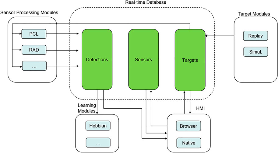
FIGURE 2. Real-time database and parallelized simulation of active-passive sensor processing, target, learning and HMI modules. For the sake of simplicity many auxiliary modules such as wave propagation, and digital elevation modules etc. are not illustrated.

5.3 Transmitters of Opportunity for PCL Sensors

We use freely available data on the FM and DAB transmitters that have been coordinated in accordance with the Geneva Plan (GE84) and licensed by the Swiss Federal Office of Communications². This data is available in machine-readable form in “.csv” and “.xml” format and includes transmitter attributes like position in geographic and national coordinates, name, frequency, bandwidth, Effective Radiated Power (ERP), horizontal antenna diagram, vertical antenna diagram etc. We use the horizontal and vertical antenna diagrams to approximate the 3D radiation pattern. When no antenna diagrams were available an omnidirectional antenna was assumed.

5.4 Topography Model

We use the Global Multi-resolution Terrain Elevation Data³ topographical data at 7.5 arc-seconds resolution with Root Mean Square Error range between 26 and 30 m.

5.5 Electromagnetic Wave Propagation Model

We have integrated the open source ⁵ library into our simulation suite BURST both Longley-Rice and ITWOM RF propagation models to compute the terrain propagation loss for the spectrum between 20 MHz and 20 GHz. Atmospheric refraction is considered using the 4/3 Earth radius model.

6 Hebbian Learning of Sensor Efficiency

Hebbian learning is widely accepted in the fields of psychology, neurology, and neurobiology as a neuroscientific theory of synaptic plasticity based on the premise that repeated stimulation of pre- and postsynaptic cells lead to increase in synaptic efficacy (Hebb, 1949). As an unsupervised learning method Hebbian learning models and its variants have been used widely in engineering and computation (Gerstner and Kistler, 2002). In contrast to learning techniques that rely on large volumes of labeled data to build the initial composition of the network (e.g. using error backpropagation in supervised learning), Hebbian learning is unsupervised and more similar to the mostly observational model employed by the animal brain in any learning activity.

We here formulate the Hebbian learning for our purpose as follows [adapted from (Gerstner and Kistler, 2002)]. The general formula for synaptic plasticity can be writte down as:

$\frac{d}{dt}{w}_{ij}=F\left(w_{ij};v_i,v_j\right)(14)$

where $\frac{d}{dt}{w}_{ij}$ is the rate of change of synaptic strength and F is a function to be defined. v_i and v_j are the post- and presynaptic neuronal firing rates respectively (for our purposes we do no need to model the membrane potentials). In order to model for the simultaneous activity of the pre- and postsynaptic neurons and the subsequent change in synaptic weight we expand the fucntion F in a Taylor series about v_i = v_j = 0:

$\frac{d}{dt}{w}_{ij}=c_0\left(w_{ij}\right)+c_i^{pre}\left(w_{ij}\right)v_j+c_1^{post}\left(w_{ij}\right)v_i+c_2^{pre}\left(w_{ij}\right)v_j^2+c_2^{post}\left(w_{ij}\right)v_i^2+c_{11}^{corr}\left(w_{ij}\right)v_i{v}_j+\mathcal{O}\left(v^3\right)(15)$

The term $c_{11}^{corr}(w_{ij})v_i{v}_j$ in Eq. 15 implements the AND condition for joint activity. The simplest choice for Hebbian learning rule within the Taylor expansion of Eq. 15 would be to fix $c_{11}^{corr}$ as a positive constant (learning rate) and set all other terms to zero. We thus get the prototypical learning rule:

$\frac{d}{dt}{w}_{ij}=c_{11}^{corr}{v}_i{v}_j(16)$

We bound the synaptic weight w_ij between 0 and 1 by making $c_{11}^{corr}$ depend on w_ij as follows:

$c_{11}^{corr}\left(w_{ij}\right)={\gamma }_1\left(1-w_{ij}\right)(17)$

In summary we obtain the learning rule

$\frac{d}{dt}{w}_{ij}={\gamma }_1\left(1-w_{ij}\right)v_i{v}_j-{\gamma }_2{w}_{ij}(18)$

where the synaptic weights are bounded and decay back to zero in the absence of stimulation. γ_i are thereby normalization factors (according to the so called Oja’s rule) which solves the typical stability problems of the Hebb’s learning rule. Besides, in the case of PCL topology learning we need to allow competition between ToOs as the computational resources per PCL sensor site are limited and the best ToOs have to be chosen. To account for this we normalize the synaptic weights w_ij for each PCL receiver. The left side of the Figure 3 illustrates the neural network for PCL topology optimization. Each PCL receiver is modelled as a presynaptic neuron that is connected through a synapse to all the potentially available ToOs. The synaptic weights w_ij will be learned according to the above rule. The right side of the Figure 3 illustrates the neural network for active radar power budget and sector optimization. Each active radar is modelled by a presynaptic neuron that is connected to all nodes in a 2D postsynaptic neural matrix. The two dimensions of the 2D postsynaptic neural matrix represent all potentially available sectors and ranges of active radars used in the simulation. Note that further dimensions can be added if necessary.

FIGURE 3

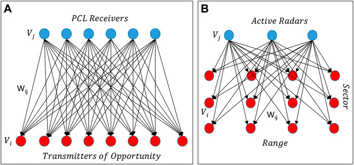
FIGURE 3. (A) PCL single layered neural network for Hebbian learning. Both the input (PCL receivers as blue circles) and output layers (ToOs as red circles) are one dimensional. (B) Active radar power budget and sector utility learning neural network for Hebbian learning. Input layer has as nodes active radars (blue circles). The output layer (red circles) is two dimensional accounting for the sensor range and sectors.

Given the above discussed neural architecture for Hebbian learning we now discuss the pre- and postsynaptic activation functions. Using the BURST simulation suite presented in section 5.1 we simultaneously simulate targets and their detection using PCL and active radars in an RSN. The simulated targets are recorded real-world air traffic using either ADS-B or combined military and civil air surveillance radars. Whenever a sensor detects a target the following activation function is triggered in the neural network for both pre- and postsynaptic PCL neurons for receiver j and ToO i:

$v_i=v_j=S\left(x\right)=\frac{1}{1+e^{-x}}(19)$

where S is the sigmoid function and x a specific detected target is given by:

$x=f\left(i,j,target\right)=\left\{\begin{array}{cc}1.0-\frac{a}{b}-\frac{c}{d}\hfill & \text{if}Receive{r}_j\text{and}To{O}_i\text{detects}target\hfill \\ 0\hfill & \text{otherwise}\hfill \end{array}\right.(20)$

where a is the total number of PCL detections, b is total number of PCL sensors (where each PCL receiver-ToO couple is defined as a sensor), c is the total number of active radar detections and d total number of active radars. This activation function states on the one hand that the more unique the detection of a target by a given receiver-transmitter pair (i.e. PCL sensor) the higher the activity. The uniqueness of a detection by a PCL sensor is thereby given by $1-\frac{a}{b}$, which will be 0 if all PCL sensors detect this same target and close to 1 if only the current PCL sensor detects it. On the other hand Eq. (20) also states that the higher the number of active radar detections of the same target (c) the lesser the activity for this PCL sensor. This formulation of the activity function rewards the most useful (i.e unique) PCL detections as these detections cannot be provided by the other passive or active sensors in the RSN.

Analogously for active radars, the active activation function for radar i is defined as follows:

$x=f\left(i,target\right)=\left\{\begin{array}{cc}1.0-\frac{c}{d}\hfill & \text{if}\text{target\hspace{0.17em}not\hspace{0.17em}detected\hspace{0.17em}by\hspace{0.17em}any\hspace{0.17em}PCL\hspace{0.17em}sensor}\hfill \\ 0\hfill & \text{otherwise}\hfill \end{array}\right.(21)$

This formulation allows us to reward PCL sensors that detect targets that are rather undetected by other PCL sensors and by active radars. Also, active radar detections are considered as valuable where there is no PCL detection. This allows the aforementioned exploitation of the added value of PCL sensors are gap fillers in an active-passive RSN.

In the case of active radars, the same formulation as in Eq. (20) is used rewarding reciprocally the ranges and sectors where each active radar has the most unique detection contributions. Note that in case the value of x in Eq. (20) is below zero, the learning rule in Eq. (18) leads to the depression of the corresponding synaptic weight, which can be compared to forgetting in the biological brain. This is useful as negative values of x in Eq. (20) is caused when a lot of sensors detect the same target at its position, which is unnecessarily redundant when the objective is to maximize RSN coverage in space.

The formulation of our learning problem as a Hebbian network illustrated in Figure 3 allows us to show the geographic distribution of active radar synaptic weights in azimuth-range plots with the active radar at the centre (range = 0). Such results will be discussed in section 7 in Figures 8–10.

7 Results

We compared the three following scenarios with each other to quantify the added value of our approach. First we considered a scenario with merely three active radars (further named scenario one). Secondly we considered the same three active radars and one FM passive radar (scenario two). As the third scenario we considered the same active and passive radars as in scenario two, but with only foreign (i.e. non Swiss) FM transmitters of opportunity for the passive radar (scenario three). Firstly this allows to show the resource allocation optimization possibility when integrating a passive radar into a given active radar set up (scenario one compared to scenario two). And further scenario three allows to demonstrate the versatility of our approach to demonstrate the degradation in resource savings achieved above if the Swiss FM transmitters are to be shut down in the next years as currently planned by the Swiss regulators.

All PCL and active radar parameters and locations are arbitrary and unclassified. The PCL sensor uses eleven FM transmitters within and outside Switzerland (scenario two) and six non Swiss FM transmitters (scenario three). Eleven strongest FM transmitters were chosen from all retrieved from the publicly available BAKOM dataset (BAKOM). FM transmitter attributes available from the dataset were position (lat, lon), antenna height above ground, frequency, power, bandwidth, horizontal radiation pattern, vertical radiation pattern and polarisation. The computed coverage for the PCL sensor using all eleven ToOs is shown in Figure 4. The computed coverage for the PCL sensor using only foreign ToOs is shown in Figure 5.

FIGURE 4

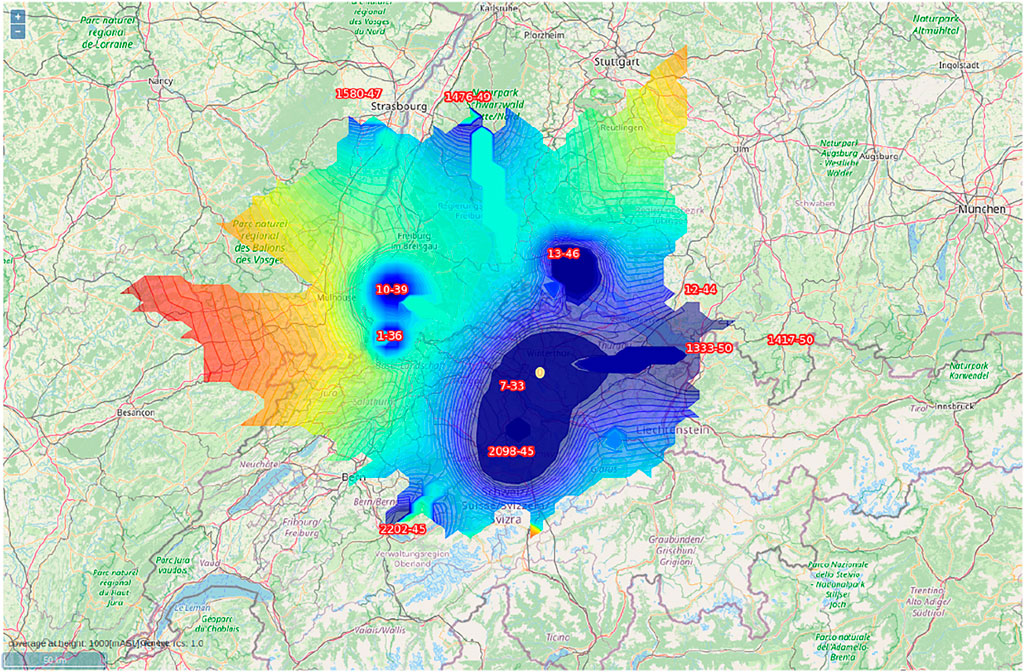
FIGURE 4. Passive Radar Coverage using all ToOs: FM Sensor is shown as the yellow circle and real world FM transmitters as red numbers. Coverage computation is shown as minimal detectable RCS (0.1 blue to 150 m² red) for altitude 3000 masl.

FIGURE 5

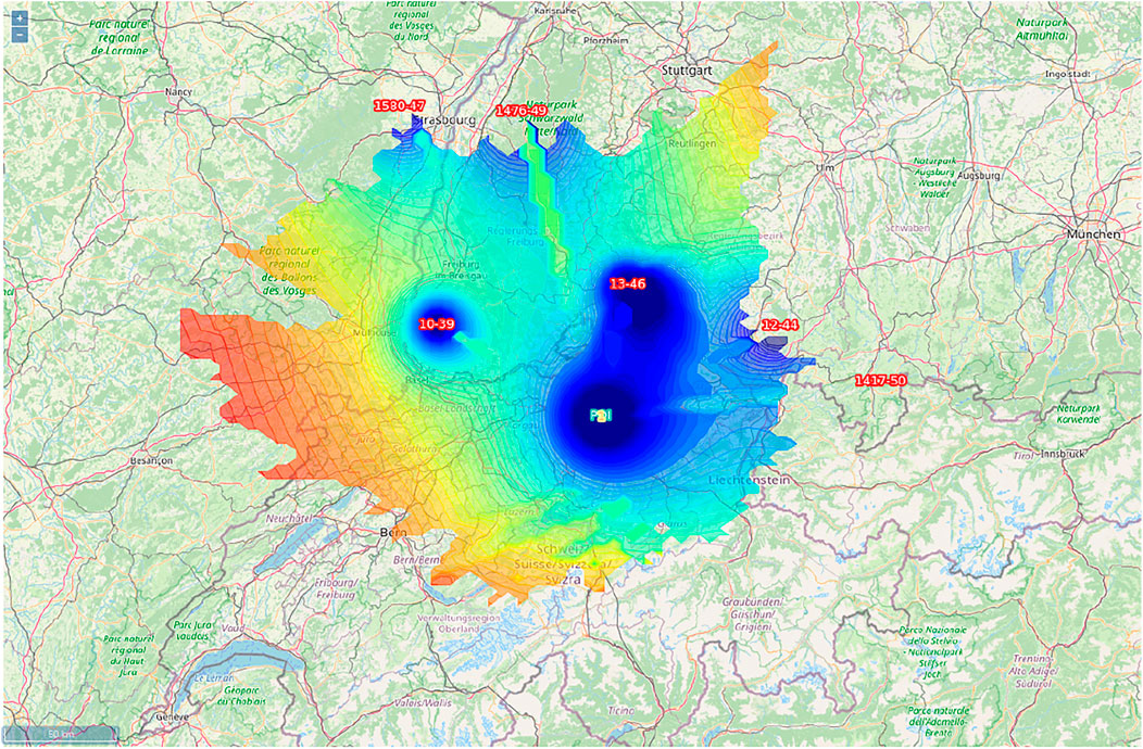
FIGURE 5. Passive Radar Coverage using non-Swiss ToOs: FM Sensor is indicated by the yellow circle and real world FM transmitters outside Switzerland by red numbers. Coverage computation is shown as minimal detectable RCS (0.1 blue to 150 m² red) for altitude 3000 masl.

For resource optimization using Hebbian learning ADS-B air traffic recording during a 2 hour period above continental Europe were used to simulate real-world targets.

The active radar parameters used for target detection were: lat, lon, height, power, antenna diameter, frequency, pulsewidth, number of integrated pulses, and bandwidth. The probability of false alarm and rotation time of all active radars were set to 10^–6 and 4 s respectively. The above active radar parameters were set so that a detection range of about 80 kms were achieved for a target of 10 m² RCS. Figure 6 for the coverage prediction of all three active radars at altitude 3000 masl.

FIGURE 6

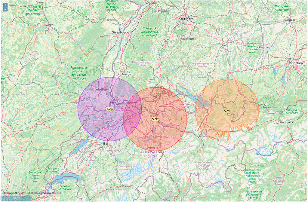
FIGURE 6. Three active Radars (numbers 524, 525, 526) with coverage illustrations as probability of detection greater than 0.8 for a target of 10 m² RCS at 3000 masl.

Figure 7 illustrates the antenna diagrams of two real world FM transmitters.

FIGURE 7

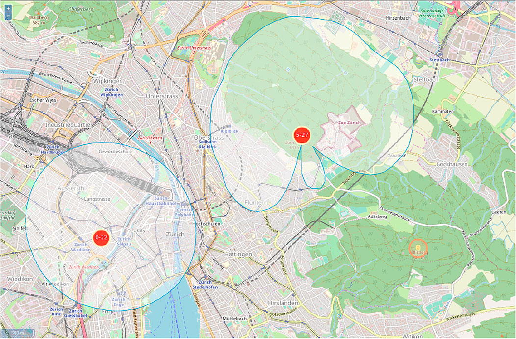
FIGURE 7. Two real-world FM transmitters (red circles) with the corresponding horizontal antenna radiation patterns.

Figures 8–10 illustrate the results of the proposed learning mechanism to minimize active radar power budget for providing target coverage for the mentioned real-world target scenario of 2 hour duration. Figures 8–10 illustrate the synaptic weights of active radars after the convergence of the Hebbian learning mechanism. The heat map color coding indicates high synaptic weights to low synaptic weights from red to blue respectively. Each of these Figures shows three active radars discussed in Figure 6 in the middle of each subplot. For example a high synaptic weight after learning (color coded red) at a given azimuth and range from a radar indicates that the contribution of this specific radar in detecting targets at this azimuth and range is high. Likewise a low synaptic weight (blue) indicates irrelevant contribution of this radar at this azimuth and range.

FIGURE 8

FIGURE 8. Scenario 1: Active Radar Only: learned normalized weights of the three active radars in an azimuth-range polar plot are shown. A mean weight of 80% (83 + 84 + 73)/3 is obtained, meaning that on average targets in 80% of the range-sector bins are detected.

FIGURE 9

FIGURE 9. Scenario 2: Active Radar and Passive Radar with all 11 ToOs: learned normalized weights of the three active radars in an azimuth-range polar plot are shown. A mean weight of 33% (61 + 22 + 16)/3 is obtained, more than halving the active radar only mean synaptic weight in scenario 1. Hereby, cold (blue) areas indicate low synaptic weights where active radar detection is made unnecessary thanks to detections of the PCL sensor.

FIGURE 10

FIGURE 10. Scenario 3: Active Radar and Passive Radar with only six non Swiss ToOs: learned normalized weights of the three active radars in an azimuth-range polar plot are shown. For the three active radars a mean weight of 46% (65 + 48 + 27)/3 is obtained, which means increment of 13% compared to scenario 2.

By comparing Figure 8 (scenario 1) with Figure 9 (scenario 2) we observe that the relative contributions of all three active radars in scenario two is much lower than that in scenario 1. Quantitatively this is shown by the mean synaptic weight of 33% in scenario two compared to 80% in scenario 1. This means that by adding a single PCL sensor to the three active RSN group we can drastically reduce the critical coverage requirement of active radars for providing the same air picture (i. e. while maintaining the detection sensitivity). It has to be noted that a typical real-world PCL system possibly cannot provide the same 3D position accuracy as a 3D active radar depending on the used ToO signal bandwidth and the relative geometry of the receiver, ToOs and targets. Furthermore it has to be noted that synpatic weight at lower range is irrelevant when the weight at a greater range is high. In such cases the active radar has to illuminate indeed all ranges in a sector. The added value of the learning mechanism is when complete sectors can be singled out that need not be illuminated (e.g. Figure 9 middle 0–90° azimuth).

By comparing Figure 10 (scenario 3) with Figure 9 (scenario 2) we observe that the mean synaptic weight of active radars is raised from 33 to 46% when the PCL sensor uses just ToOs outside Switzerland. This means that although the usage of CH inland FM ToOs do contribute to the PCL air picture, a significant part of that air picture can be provided by using just ToOs outside Switzerland. This again means that PCL FM sensors in Switzerland would be useful even if the FM transmitters were to be shut down in the near future. Note that the result in Figure 10 owing to scenario three was achieved dynamically from scenario two shown in Figure 9 by simply switching off the Swiss FM transmitters. This transition in the learned synaptic weights shows that our approach can relearn dynamically.

Figures 11, 12 illustrate how the same Hebbian learning mechanism is used to learn the most useful ToOs, i.e. the ones contributing to the most number of target detections. For this we consider scenario 2. Figure 11 illustrates how the synaptic weights of individual ToOs develop over the learning epochs. Figure 12 summarizes these ToO synaptic weights in boxplots. Here we see that there are four ToOs with considerably more contributions to target detections than the others. This learned result can be used by a PCL system to prioritize processing of ToOs as often computational resources are limited especially for mobile PCL systems operating in harsh alpine conditions.

FIGURE 11

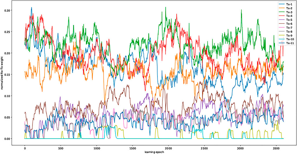
FIGURE 11. Normalized learned weights of individual ToOs over learning epochs when all 11 (both Swiss and foreign) FM transmitters are used. The ToOs with higher weights contribute to much more detections than the ToOs with low weights.

FIGURE 12

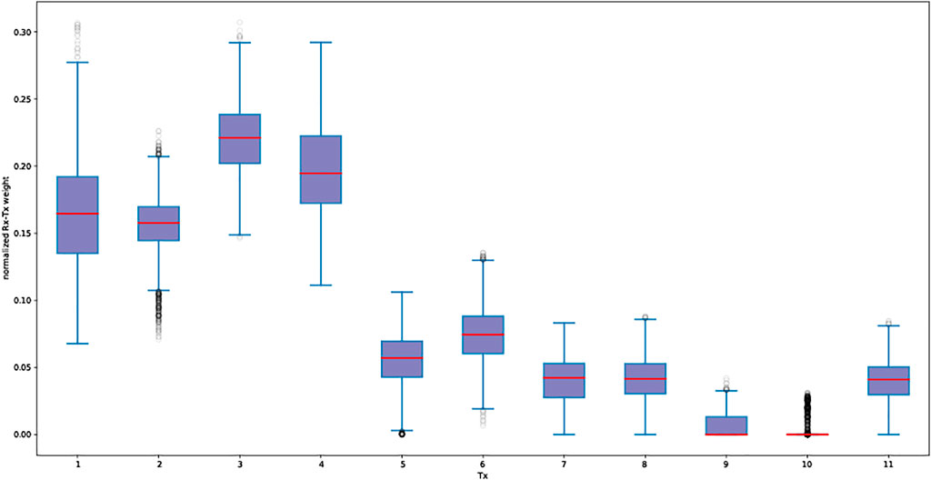
FIGURE 12. Boxplots of individual ToO weights after learning when all 11 (both Swiss and foreign) FM transmitters are used. The ToOs with higher weights can be clearly distinguished from the ToOs with low weights.

8 Conclusion

Given a set of active radars and PCL sensors on certain locations, we addressed the problem of simultaneously determining the most useful ToOs for each PCL sensor and the most effective sectors and ranges for each active radar. From this optimal power budget strategies (e. g avoiding emissions in some sectors) can easily be derived. We proposed an unsupervised learning approach for this topology optimization and energy-efficient detection in combined active-passive radar sensor networks. Our approach shows how and where the power budget of active radars can be drastically minimized by introducing PCL sensors. Although PCL systems seem promising as cost-effective gap fillers of active radar coverage they are sensitive to changes of ToO. To this end we demonstrated how our approach dynamically relearns to achieve robust performance when changes in the ToO of PCL sensors occur. The most useful ToOs for PCL target detection are learned while providing a means to select sectors of no emission for active radars, and thus for minimizing their power budgets.

Our approach critically contributes towards the goal of minimizing active radar power budget and PCL computational resources in a RSNs. Widely used approaches to attack power budget optimization in RSNs include game-theoretic approaches and network cost based strategies, which mostly do not consider detailed models of active and passive radars and terrain models. Our approach using Hebbian learning allows to integrate user defined models of PCL and active radar systems. Furthermore, our approach allows scenario dependent optimization of active radar power budget and PCL ToO selection. Recordings of real-world air traffic, simulated targets or a combination of both can be used to train our model catering to several scenarios in military and civilian air surveillance.

Further work is envisioned to consider more sophistic models of PCL and active radar detection models including bistatic RCS modelling, clutter modelling, direct signal suppression and digital beamforming.

Data Availability Statement

The datasets presented in this article are not readily available because of applicable data clearance procedures at the authors’ institutions. Requests to access the datasets should be directed to the corresponding author.

Author Contributions

ZM conceived, modelled and implemented the learning algorithm. The simulation framework was designed and implemented by ZM and LQ. CS and PW provided useful inputs to the model and the simulation framework. ZM performed the simulation tests. All authors contributed to the writing of the manuscript.

Conflict of Interest

The authors declare that the research was conducted in the absence of any commercial or financial relationships that could be construed as a potential conflict of interest.

Publisher’s Note

All claims expressed in this article are solely those of the authors and do not necessarily represent those of their affiliated organizations, or those of the publisher, the editors and the reviewers. Any product that may be evaluated in this article, or claim that may be made by its manufacturer, is not guaranteed or endorsed by the publisher.

Footnotes

¹The scenario described in this work comprises of arbitrary sensor locations, parameters and coverages, which were chosen solely to explain the proposed learning approach and therefore have no operational relevance in the Swiss Air Force defense scenario.

²(Dataset) BAKOM (). https://www.bakom.admin.ch/bakom/en/homepage/frequencies-and-antennas/location-of-radio-transmitters.html.

³(Dataset) GMTED (). https://www.usgs.gov/products/data-and-tools/gis-data.

⁴(Dataset) POSTGRESQL (). https://www.postgresql.org/.

⁵(Dataset) SPLAT! (). https://www.qsl.net/kd2bd/splat.html.

References

Bacci, G., Sanguinetti, L., Greco, M. S., and Luis, M. (2012). “A Game-Theoretic Approach for Energy-Efficient Detection in Radar Sensor Networks,” in IEEE 7th Sensor Array and Multichannel Signal Processing Workshop (SAM) (IEEE), 157–160. doi:10.1109/sam.2012.6250454

CrossRef Full Text | Google Scholar

Baker, C. J., and Hume, A. L. (2003). Netted Radar Sensing. IEEE Aerosp. Electron. Syst. Mag. 18, 3–6. doi:10.1109/maes.2003.1183861

CrossRef Full Text | Google Scholar

Baker, C. J., and Trimmer, B. D. (2000). Short-range Surveillance Radar Systems. Commun. Eng. J. 12, 181–191. doi:10.1049/ecej:20000406

CrossRef Full Text | Google Scholar

Barton, D. (2013). Modern Radar Systems Analysis. Norwood, MA: Artech House.

Google Scholar

Gerstner, W., and Kistler, W. M. (2002). Mathematical Formulations of Hebbian Learning. Biol. Cybern 87, 404–415. doi:10.1007/s00422-002-0353-y

PubMed Abstract | CrossRef Full Text | Google Scholar

Griffiths, H., and Baker, C. (2005). Passive Coherent Location Radar Systems. Part 1: Performance Prediction. IEE Proc. Radar Sonar Navigation 152, 1. doi:10.1049/ip-rsn:20045082

CrossRef Full Text | Google Scholar

Hebb, D. (1949). The Organization of Behavior. New York: New York: Wiley & Sons.

Google Scholar

Jackson, M. C. (1986). The Geometry of Bistatic Radar Systems. IEE Proc. F Commun. Radar Signal. Process. UK 133, 604–612. doi:10.1049/ip-f-1.1986.0097

CrossRef Full Text | Google Scholar

Jiang, X., Yi, W., Yuan, Y., Chai, L., and Zhang, X. (2019). “Network Cost Based Node Selection Strategy for Multiple Target Tracking in Netted Radar System,” in IEEE Radar Conference (IEEE). doi:10.1109/radar.2019.8835509

CrossRef Full Text | Google Scholar

Malanowski, M., Zywek, M., Plotka, M., and Kulpa, K. (2022). Passive Bistatic Radar Detection Performance Prediction Considering Antenna Patterns and Propagation Effects. IEEE Trans. Geosci. Remote Sensing 60, 1–16. doi:10.1109/TGRS.2021.3069636

CrossRef Full Text | Google Scholar

Mathews, Z., Quiriconi, L., and Weber, P. (2015). “Multi-static Passive Receiver Location Optimization in alpine Terrain Using a Parallelized Genetic Algorithm,” in 2015 IEEE Radar Conference (RadarCon) (IEEE), 1446–1451. doi:10.1109/RADAR.2015.7131222

CrossRef Full Text | Google Scholar

Mousel, P. (2017). “Passive Radar: From Quality Criteria to Coverage Optimization,” in Master Thesis ETH Zürich (Zürich, Switzerland: ETH Zürich).

Google Scholar

Schreiner, B. (1999). A Matlab Radar Range Equation and Probability of Detection Evaluation Tool. Adelphi, MD: Army Research Lab.

Google Scholar

Skolnik, M. (1980). Introduction to Radar Systems. London: McGraw-Hill.

Google Scholar

Yi, J., Wan, X., Leung, H., and Lü, M. (2017). Joint Placement of Transmitters and Receivers for Distributed Mimo Radars. IEEE Trans. Aerosp. Electron. Syst. 53, 122–134. doi:10.1109/TAES.2017.2649338

CrossRef Full Text | Google Scholar