CRLBs for Location and Velocity Estimation for MIMO Radars in CES-Distributed Clutter

In this article, we investigate the problem of jointly estimating target location and velocity for widely separated multiple-input multiple-output (MIMO) radar operating in correlated non-Gaussian clutter, modeled by a complex elliptically symmetric (CES) distribution. More specifically, we derive the Cramér–Rao lower bounds (CRLBs) when the target is modeled by the Swerling 0 model and the clutter is complex t-distributed. We thoroughly analyze the impact of the clutter correlation and spikiness to provide accurate performance estimation. Index terms—Cramér–Rao lower bounds (CRLBs), MIMO radar, location and velocity estimation, performance analysis, complex elliptically symmetric (CES) distributed, and complex t-distribution.

1 Introduction

Multiple-input multiple-output (MIMO) radars have attracted increasing attention in recent years, as proved by the many published articles (see, for instance, Fishler et al., 2004; Li and Stoica, 2008; Davis, 2015). MIMO radars can be classified as coherent or noncoherent (He et al., 2010a; Derham et al., 2010), and colocated (Li and Stoica, 2007) or widely distributed (Haimovich et al., 2007).

Estimating target parameters in MIMO radars is one of the far-reaching research topics; hence, various research studies have considered different scenarios, with different antenna deployment (Fishler et al., 2006; Li and Stoica, 2009), target models (in motion or static target) (Hassanien et al., 2012), and various estimation algorithms (Stoica and Nehorai, 1990; Tajer et al., 2010; Min et al., 2011). The Cramér–Rao lower bound (CRLB) is a well-known tool for evaluating target parameter estimation performance in clutter. In Godrich et al., (2008a), Godrich et al., (2010), the CRLBs were derived for target localization in noncoherent and coherent MIMO radars. The CRLB for target velocity was presented in He et al., (2010b), while the CRLB for joint estimation of target location and velocity in case of noncoherent MIMO radars was derived in He et al., (2010a). In Godrich et al., (2008b), He et al., (2008), CRLBs were derived for MIMO radars with widely separated antennas.

In all the cited articles, the clutter is modeled as a Gaussian stochastic process, white or colored. Such assumption is a good approximation in many cases, but not always, particularly when the clutter is very spiky, for e.g., in high resolution radars (Brekke et al., 2010). In MIMO radars, sometime the clutter has been modeled as a non-Gaussian process by the compound-Gaussian (CG) (Farina et al., 1997; Gini, 1998; Gini and Greco, 1999; Sangston et al., 1999; Sangston et al., 2012) or the complex elliptically symmetric (CES) distributions (Ollila et al., 2012; Fortunati et al., 2019) that include a wide variety of distributions such as complex normal (CN) (Goodman, 1963), complex generalized Gaussian (Novey et al., 2009), complex-t $(\mathbb{C}t)$, complex-k, and all the other CG distributions (Krishnaiah and Lin, 1986; Zhang et al., 2014; Zhang et al., 2017).

The novel contribution of this article is to derive the CRLBs on the estimation of location and velocity under the assumption that the non-Gaussian correlated clutter is modeled by a $\mathbb{C}t$-distribution. We then analyze the impact of the clutter correlation and spikiness on the estimation performance.

This article is organized as follows: the data model is described in Section 2. In Section 3, the general CES model and the complex t-distribution are summarized. In Section 4, we derive the analytical expression of the CRLBs for the estimation of target location and velocity, and some numerical results are reported in Section 5 to investigate the theoretical findings.

2 Data Model

Consider a coherent MIMO radar with M transmit (TX) and N receive (RX) antennas, widely dispersed in a 2-D plane as shown in Figure 1. In order to simplify the CRLB derivation of target location and velocity, we assume an isotropic target whose unknown complex amplitude is ζ = ζ_R + jζ_I. The unknown target location is (x, y), and the unknown target velocity is (v_x, v_y). The known locations of the M transmitters are $(x_k^t,y_k^t),(k=1,\dots ,M)$ and of the N receivers are $(x_l^r,y_l^r),(l=1,\dots ,N)$. ϕ_k is the orientation of the kth transmitter, and φ_l is the orientation of the lth receiver with respect to the x − axis.

FIGURE 1

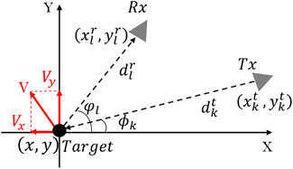
FIGURE 1. Transmitters and receivers location with respect to the moving target.

The echo at the lth receiver from the transmission of all the M transmitters and reflected from the target, after down-conversion and sampling, is

$\begin{array}{c}{r}_l\left[n\right]=\sqrt{\frac{E}{M}}\mathrm{\zeta }\sum _{k=1}^M{e}^{-j2\mathrm{\pi }{f}_0{\tau }_{lk}}{e}^{j2\mathrm{\pi }{f}_{lk}n{T}_s}{s}_k\left(n{T}_s-{\tau }_{lk}\right)+z_l\left[n\right],\\ l=1,\dots ,Nn=1,\dots .,N_s\end{array},(1)$

where ζ is the target complex reflectivity (unknown and deterministic), f₀ is the carrier frequency (carrier frequencies of all transmitters are assumed to be identical), T_s is the sampling time (chosen to satisfy the Nyquist criterion), and N_s is the number of samples in the observation period, $s_k({\mathrm{\Delta }}_n)=\mathrm{f}({\mathrm{\Delta }}_n)\cdot \mathrm{r}\mathrm{e}\mathrm{c}\mathrm{t}(\frac{{\mathrm{\Delta }}_n}{T_p})$ with Δ_n = (nT_s − τ_lk), which is the complex baseband signal received by the lth receiver sent by the kth transmitter. The $\mathrm{r}\mathrm{e}\mathrm{c}\mathrm{t}(\frac{{\mathrm{\Delta }}_n}{T_p})$ models the single pulse time interval, while f(Δ_n) refers to the specific class of signal implementation, and T_p refers to the pulse duration. Each signal is emitted by an individual transmitter antenna with energy E_s, while E = E_sM is the total transmitted energy. Finally, z_l[n] is the clutter echo at the lth receiver.

τ_lk represents the time delay of a signal given by

${\tau }_{lk}=\frac{d_k^t+d_l^r}{c},(2)$

where $d_k^t=\sqrt{{(x_k^t-x)}^2+{(y_k^t-y)}^2}$ is the path from the kth TX antenna to the target, $d_l^r=\sqrt{{(x_l^r-x)}^2+{(y_l^r-y)}^2}$ is the path from the target to the lth RX antenna, and c indicates the speed of light.

f_lk is the target Doppler frequency shift given by

$f_{lk}=\frac{v_x\left(x_k^t-x\right)+v_y\left(y_k^t-y\right)}{\mathrm{\lambda }{d}_k^t}+\frac{v_x\left(x_l^r-x\right)+v_y\left(y_l^r-y\right)}{\mathrm{\lambda }{d}_l^r},(3)$

where λ indicates the wavelength of the carrier frequency.

In our derivation, we assume that the transmitted signals are orthogonal (Peilin Sun et al., 2014). Furthermore, they retain approximately orthogonality, even after a variety of allowed time delays and Doppler frequency shifts, that is,

$\begin{array}{c}\sum _{n=1}^{Ns}{s}_k\left(n{T}_s-{\tau }_{lk}\right)s_{k^{\prime }}^{*}\left(n{T}_s-{\tau }_{l^{\prime }{k}^{\prime }}\right)e^{j2\pi \left(f_{lk}-f_{l^{\prime }{k}^{\prime }}\right)n{T}_s}\\ \left\{\begin{array}{c}1ł=l^{\prime },k=k^{\prime }\hfill \\ 0ł\ne l^{\prime },k\ne k\hfill \end{array}\right.\forall {\tau }_{lk},f_{lk},{\tau }_{l^{\prime }{k}^{\prime }},f_{l^{\prime }{k}^{\prime }}\end{array}.(4)$

The orthogonality as given in Eq. 4 is clearly a strong condition if applied to all possible delays and Doppler frequencies. Despite this, for reasonable values of Doppler frequencies and the set of target and radar parameters of this work, we verified that the cross-ambiguity functions are negligible compared to the auto-ambiguity functions; thus, the orthogonal condition can be considered approximately met.

Finally, the N_s-dimensional observation vector at the lth receiver can be expressed as ${\mathbf{r}}_l={\left\{\begin{array}{cccc}\hfill r_l[1]\hfill & \hfill r_l[2]\hfill & \hfill \dots \hfill & \hfill r_l[N_s]\hfill \end{array}\right\}}^T$.

3 Complex Elliptically Symmetric Distribution

Complex elliptically symmetric (CES) distributions are commonly used to model non-Gaussian heavy-tailed radar clutter (Zhang et al., 2014; Fortunati et al., 2018; Fortunati et al., 2019; Raninen et al., 2021). The m-variate random vector (r.v) $\mathbf{z}\in {\mathbb{C}}^m$ that follows the CES model has a probability density function (pdf) of the form,

$f_z\left(\mathbf{z}\right)=C_{m,g}{\left|\mathbf{\Sigma }\right|}^{-1}g\left({\left(\mathbf{z}-\mathit{\mu }\right)}^H{\mathbf{\Sigma }}^{-1}\left(\mathbf{z}-\mathit{\mu }\right)\right),(5)$

where $\mathit{\mu }\in {\mathbb{C}}^m$ and the m × m matrix Σ denote the symmetry center and scatter matrix, respectively. The function g: $R_0^{+}\to R^{+}$, called density generator function, satisfies the constraint ${\delta }_{m,g}\triangleq {\int }_0^{\infty }{t}^{m-1}g(t)dt<\infty$, and (.)^H refers to the Hermitian (complex conjugate and transpose) operator. C_m,g is a normalizing coefficient such that f_z(z) integrates to 1 and $C_{m,g}=2{(S_m{\delta }_{m,g})}^{-1}$, where $S_m\triangleq \frac{2{\mathrm{\pi }}^m}{\mathrm{\Gamma }(m)}$.

Then, the clutter can be represented in short notation by

$z\sim C{E}_m\left(\mathit{\mu },\mathbf{\Sigma },g\right)=C{E}_{m,g}\left(\mathit{\mu },\mathbf{\Sigma }\right).(6)$

3.1 t-Distributed Clutter

A particular case of CES-distributions is the $\mathbb{C}t$-distribution (Krishnaiah and Lin, 1986; Ollila et al., 2012), in short notation z ∼ Ct_m,ν(μ, Σ).

For a complex t-distribution of dimension m, the generating function is given by

$g\left(t\right)={\left(1+\frac{2t}{\mathrm{\nu }}\right)}^{\frac{-\left(2m+\mathrm{\nu }\right)}{2}}(7)$

and $C_{m,g}=\frac{2^m\mathrm{\Gamma }(\frac{2m+\mathrm{\nu }}{2})}{{(\mathrm{\pi }\mathrm{\nu })}^m\mathrm{\Gamma }(\frac{\mathrm{\nu }}{2})}$ is the normalizing constant. ν is the shape parameter of the distribution, and it is related to the spikiness of the clutter. The lower the value of ν, the spikier is the clutter (Sangston et al., 2012). For ν → ∞, the t-distribution degenerates into the Gaussian one.

Here, we investigate two different scenarios for the clutter. Model I: the clutter samples are uncorrelated in space and time. Model II: the clutter samples are temporally uncorrelated but spatially correlated. The mean value is 0, that is, μ = 0.

4 The Joint Cramér–Rao Lower Bound

The CRLB provides a lower bound of the variance of any unbiased estimator of unknown deterministic parameters. Given ψ = [x, y, v_x, v_y, ζ_R, ζ_I] as the vector of all the unknown parameters in the received signal, we derive the CRLBs for the MIMO radar. Since we assume here that the target has already been detected and we want to estimate target range and velocity, we consider the target reflectivity, ζ_R and ζ_I, as nuisance parameters (Gini and Reggiannini, 2000; Fortunati et al., 2010), then we derive the CRLBs of the unknown vector β_p×1 = [x, y, v_x, v_y], p = 4.

4.1 CRLB for Target Range and Velocity

In order to derive the CRLB of target location and velocity, the first step is to calculate the Fisher information matrix (FIM) and then to invert it, CRLB(ψ) = [J(ψ)]⁻¹.

The FIM matrix is defined as

${\left[\mathbf{J}\left(\mathbf{\psi }\right)\right]}_{i,j}=-E_{\mathbf{r},\mathbf{\psi }}\left\{\frac{\partial }{\partial {\mathbf{\psi }}_i}\left[\frac{\partial }{\partial {\mathbf{\psi }}_j}lnp\left(\mathbf{r};\mathbf{\psi }\right)\right]\right\},(8)$

where E{.} indicates the expectation operator, ln p(r; ψ) is the log-likelihood (LL) function, and r is the data vector. The FIM is a p × p symmetric positive semi-definite matrix after deleting the rows and columns of the nuisance parameter.

Since (1) is a function of time delay and Doppler frequency shift, we introduce the (2 + NM)-dimensional parameter vector $\mathbf{\Theta }={[{\tau }_{11},{\tau }_{12},\dots ,{\tau }_{lk},f_{11},f_{12},\dots ,f_{lk},{\zeta }_R,{\zeta }_I]}^T$, and since ψ is a function of Θ, in order to compute the FIM, the chain rule (He et al., 2010a) is applied; therefore, the FIM can be expressed as

$\mathbf{J}\left(\mathbf{\psi }\right)=\mathbf{P}\mathbf{J}\left(\mathbf{\Theta }\right){\mathbf{P}}^T,(9)$

where $\mathbf{P}=\frac{\partial {\mathbf{\Theta }}^T}{\partial \mathbf{\psi }}$ depends on the geometry of the scenario and is given by

$\begin{array}{l}\hfill \mathbf{P}=\frac{\partial {\mathbf{\Theta }}^T}{\partial \mathbf{\psi }}=\left[\begin{array}{cc}\hfill {\mathbf{U}}_{4\times 2NM}\hfill & \hfill {\mathbf{0}}_{4\times 2}\hfill \\ \hfill {\mathbf{0}}_{2\times 4}\hfill & \hfill {\mathbf{I}}_2\hfill \end{array}\right],\end{array}(10)$

where 0 and I are the zero and identity matrices, respectively, while U is given by

$\mathbf{U}=\left[\begin{array}{cccccc}\hfill \frac{\partial {\tau }_{11}}{\partial x}\hfill & \hfill \dots \hfill & \hfill \frac{\partial {\tau }_{NM}}{\partial x}\hfill & \hfill \frac{\partial f_{11}}{\partial x}\hfill & \hfill \dots \hfill & \hfill \frac{\partial f_{NM}}{\partial x}\hfill \\ \hfill \frac{\partial {\tau }_{11}}{\partial y}\hfill & \hfill \dots \hfill & \hfill \frac{\partial {\tau }_{NM}}{\partial y}\hfill & \hfill \frac{\partial f_{11}}{\partial y}\hfill & \hfill \dots \hfill & \hfill \frac{\partial f_{NM}}{\partial y}\hfill \\ \hfill 0\hfill & \hfill \dots \hfill & \hfill 0\hfill & \hfill \frac{\partial f_{11}}{\partial v_x}\hfill & \hfill \dots \hfill & \hfill \frac{\partial f_{NM}}{\partial v_x}\hfill \\ \hfill 0\hfill & \hfill \dots \hfill & \hfill 0\hfill & \hfill \frac{\partial f_{11}}{\partial v_y}\hfill & \hfill \dots \hfill & \hfill \frac{\partial f_{NM}}{\partial v_y}\hfill \end{array}\right].(11)$

The details on the derivation of the elements of U are in He et al. (2010a). J(Θ) is the Jacobian matrix such that

$\begin{array}{l}\hfill {\left[\mathbf{J}\left(\mathbf{\Theta }\right)\right]}_{i,j}=-E_{\mathbf{r},\mathbf{\Theta }}\left\{\frac{\partial }{\partial {\mathbf{\Theta }}_i}\left[\frac{\partial }{\partial {\mathbf{\Theta }}_j}lnp\left(\mathbf{r};\mathbf{\Theta }\right.\right]\right\}.\end{array}(12)$

Matrix J(Θ), computed as in Eq. 12, can be divided into four submatrices as follows:

$\begin{array}{ll}\hfill \mathbf{J}\left(\mathbf{\Theta }\right)=& \left[\begin{array}{cc}\hfill {\mathbf{D}}_{2NM\times 2NM}\hfill & \hfill {\mathbf{G}}_{2NM\times 2}\hfill \\ \hfill {\mathbf{G}}_{2\times 2NM}^T\hfill & \hfill {\mathbf{L}}_{2\times 2}\hfill \end{array}\right],\hfill \end{array}(13)$

where $\mathbf{D}=\left[\begin{array}{cc}\hfill {\mathbf{D}}_{\mathrm{\tau }}\hfill & \hfill {\mathbf{D}}_{\mathrm{\tau }f}\hfill \\ \hfill {\mathbf{D}}_{f\mathrm{\tau }}\hfill & \hfill {\mathbf{D}}_f\hfill \end{array}\right]$ in which D_τ, D_f, and D_τf ∈ R^NM×NM. The lower right submatrix L involves the derivatives of the target complex scattering coefficient, $\mathbf{L}=\left[\begin{array}{cc}\hfill {\mathbf{L}}_{{\zeta }_R}\hfill & \hfill 0\hfill \\ \hfill 0\hfill & \hfill {\mathbf{L}}_{{\zeta }_I}\hfill \end{array}\right]$. Finally, the upper right submatrix involves the derivatives related to all parameters, time delay, the Doppler frequency, and the target complex reflectivities, then $\mathbf{G}=\left[\begin{array}{cc}\hfill {\mathbf{G}}_{\mathrm{\tau }{\zeta }_R}\hfill & \hfill {\mathbf{G}}_{f{\zeta }_R}\hfill \\ \hfill {\mathbf{G}}_{\mathrm{\tau }{\zeta }_I}\hfill & \hfill {\mathbf{G}}_{f{\zeta }_I}\hfill \end{array}\right]$.

By exploiting the chain rule for Eq. 9, the FIM of ψ is given by

$\mathbf{J}\left(\mathbf{\psi }\right)=\left[\begin{array}{cc}\hfill \mathbf{U}\mathbf{D}{\mathbf{U}}^T\hfill & \hfill \mathbf{U}\mathbf{G}\hfill \\ \hfill {\mathbf{G}}^T{\mathbf{U}}^T\hfill & \hfill \mathbf{L}\hfill \end{array}\right].(14)$

Eventually, since our aim is to calculate the CRLBs of the vector β, we get it as (He et al., 2008)

${\mathbf{C}\mathbf{R}\mathbf{L}\mathbf{B}}_{\mathbf{\beta }}={\left[\mathbf{U}\left(\mathbf{D}-\mathbf{G}{\mathbf{L}}^{-1}{\mathbf{G}}^T\right){\mathbf{U}}^T\right]}^{-1},(15)$

where the diagonal elements of the CRLB matrix represent the lower bound of the variances of the parameters of interest.

1) CRLB for Clutter Model I: If the clutter is independent in both the time and space domains, then the clutter samples z_l[n] (l = 1, … , N n = 1, … , N_s) are IID.

In this case, the log-likelihood function is given by

$\begin{array}{ll}\hfill & \ln p\left(\mathbf{r}|\mathbf{\Theta }\right)=\ln \prod _{n=1}^{N_S}\prod _{l=1}^{N}p\left(r_l\left[n\right]|\mathbf{\Theta }\right)=\hfill \\ \hfill & C+\sum _{n=1}^{N_s}\sum _{l=1}^N\ln p\left(r_l\left[n\right]|\mathbf{\Theta }\right)=C+\sum _{n=1}^{N_s}\sum _{l=1}^N\ln g\left(t_l\left[n\right]\right),\hfill \end{array}(16)$

where C is a generic constant that does not depend on the parameters of interest, and the pdf of each sample r_l[n] is given by

$p\left(r_l\left[n\right];\mathbf{\Theta }\right)=\frac{C_{1,g}}{{\sigma }^2}g\left(t_l\left[n\right]\right),(17)$

where $C_{1,g}=\frac{2\mathrm{\Gamma }(\frac{2+\nu }{\nu })}{(\pi \nu )\mathrm{\Gamma }(\frac{\nu }{2})}$, t_l[n] is the quadratic form $t_l[n]=\frac{1}{{\mathrm{\sigma }}^2}{\left|r_l[n]-\sqrt{\frac{E}{M}}\mathrm{\zeta }{u}_l[n]\right|}^2$, $u_l[n]\triangleq \sum _{k=1}^M{\mathrm{\Upsilon }}_{lk}[n]s_k[{\mathrm{\Delta }}_n]$, and ${\mathrm{\Upsilon }}_{lk}[n]=e^{-j2\pi f_0{\tau }_{lk}}{e}^{j2\pi f_{lk}n{T}_s}$ represents each element of the ϒ[n] matrix of all transmitter and receiver antennas.

Each element of the Jacobian matrix is

$\begin{array}{ll}\hfill & {\left[\mathbf{J}\left(\mathbf{\Theta }\right)\right]}_{i,j}=-E\left[\frac{{\partial }^{2}lnp\left(\mathbf{r}|\mathbf{\Theta }\right)}{\partial {\mathrm{\Theta }}_i\partial {\mathrm{\Theta }}_j}\right]=\hfill \\ \hfill & -E\left[\sum _{n=1}^{N_s}\sum _{l=1}^N\left(\frac{\stackrel{\cdot \cdot }{\mathrm{g}}\left(t_l\left[n\right]\right)}{g\left(t_l\left[n\right]\right)}-\frac{\stackrel{\cdot }{\mathrm{g}}{\left(t_l\left[n\right]\right)}^2}{g{\left(t_l\left[n\right]\right)}^2}\right)\frac{\partial t_l\left[n\right]}{\partial {\mathrm{\Theta }}_i}\frac{\partial t_l\left[n\right]}{\partial {\mathrm{\Theta }}_j}+\frac{\stackrel{\cdot }{\mathrm{g}}\left(t_l\left[n\right]\right)}{g\left(t_l\left[n\right]\right)}\frac{{\partial }^2{t}_l\left[n\right]}{\partial {\mathrm{\Theta }}_i{\mathrm{\Theta }}_j}\right]\hfill \\ \hfill & i,j=1,\dots ,2NM+2\hfill \end{array}(18)$

yielding $\left(\frac{\stackrel{\cdot }{\mathrm{g}}(t_l[n])}{g(t_l[n])}\right)=-\left(\frac{2N+\nu }{\nu }\right){\left(1+\frac{2t_l[n]}{\nu }\right)}^{-1}$, and $\left(\frac{\stackrel{\cdot \cdot }{\mathrm{g}}(t_l[n])}{g(t_l[n])}-\frac{\stackrel{\cdot }{\mathrm{g}}{(t_l[n])}^2}{g{(t_l[n])}^2}\right)=\left(2\frac{2N+\nu }{{\nu }^2}\right){\left(1+\frac{2t_l[n]}{\nu }\right)}^{-2}$, where the first derivative of g is $\stackrel{\cdot }{\mathrm{g}}(t_l[n])=\frac{\partial g[t_l]}{\partial t_l}\cdot \frac{\partial t_l[n]}{\partial \mathrm{\Theta }}$.

Note that, in computing the derivatives of the LL function with respect to the parameters in Eq. 18, we consider the orthogonality conditions in Eq. 4, and then the generic element of Eq. 18 is calculated with the derivative expressions as follows:

$\begin{array}{ll}\hfill & \frac{\partial t_p\left[n\right]}{\partial f_{lk}}=\left(\frac{4\mathrm{\pi }n{T}_s}{{\mathrm{\sigma }}^2}\sqrt{\frac{E}{M}}\mathfrak{I}\left\{\mathrm{\zeta }{\mathrm{\Upsilon }}_{lk}\left[n\right]s_k\left({\mathrm{\Delta }}_n\right)r_p^{*}\left[n\right]\right\}\right.\hfill \\ \hfill & -\left.\frac{4\mathrm{\pi }n{T}_s}{{\mathrm{\sigma }}^2}\frac{E}{M}|\mathrm{\zeta }{|}^2\mathfrak{I}\left\{{\mathrm{\Upsilon }}_{lk}\left[n\right]s_k\left({\mathrm{\Delta }}_n\right)u_p^{*}\left[n\right]\right\}\right)\mathrm{\delta }\left(l-p\right);\hfill \end{array}(19)$

$\begin{array}{ll}\hfill & \frac{{\partial }^2{t}_p\left[n\right]}{\partial f_{lk}\partial f_{l^{\prime }{k}^{\prime }}}=\left(\frac{8{\pi }^2{n}^2{T}_s^2}{\sigma }\sqrt{\frac{E}{M}}\mathfrak{R}\left\{\zeta {\mathrm{\Upsilon }}_{lk}\left[n\right]s_k\left({\mathrm{\Delta }}_n\right)\left(r_p^{*}\left[n\right]-\sqrt{\frac{E}{M}}{\zeta }^{*}{u}_p^{*}\left[n\right]\right)\right\}\right.\hfill \\ \hfill & +\left.\frac{8{\pi }^2{n}^2{T}_s^2}{\sigma }\frac{E}{M}|\zeta {|}^2\mathfrak{R}\left\{e^{-j2\pi f_0\left({\tau }_{lk}-{\tau }_{l^{\prime }{k}^{\prime }}\right)}{e}^{j2\pi \left(f_{lk}-f_{l^{\prime }{k}^{\prime }}\right)n{T}_s}{s}_k\left({\mathrm{\Delta }}_n\right)s_k^{*}\left({\mathrm{\Delta }}_n\right)\right\}\right)\hfill \\ \hfill & \mathrm{\delta }\left(l-p,l-l^{\prime },k-k^{\prime }\right),\hfill \end{array}(20)$

where the aforementioned equations represent the first and second derivatives with respect to (w.r.t.) the Doppler frequency. The derivatives w.r.t. time delay and target complex reflectivity are as follows:

$\begin{array}{ll}\hfill & \frac{\partial t_p\left[n\right]}{\partial {\tau }_{lk}}=\left(-\frac{4\mathrm{\pi }{f}_0}{{\mathrm{\sigma }}^2}\sqrt{\frac{E}{M}}\mathfrak{I}\left\{\mathrm{\zeta }{r}_p^{*}\left[n\right]{\mathrm{\Upsilon }}_{lk}\left[n\right]s_k\left({\mathrm{\Delta }}_n\right)\right\}\right.\hfill \\ \hfill & -\frac{2}{{\sigma }^2}\sqrt{\frac{E}{M}}\mathfrak{R}\left\{\zeta r_p^{*}\left[n\right]{\mathrm{\Upsilon }}_{lk}\left[n\right]{\stackrel{\cdot }{\mathrm{s}}}_k\left({\mathrm{\Delta }}_n\right)\right\}+\frac{4\pi f_0}{{\sigma }^2}\frac{E}{M}|\zeta {|}^2\mathfrak{I}\left\{u_p^{*}\left[n\right]{\mathrm{\Upsilon }}_{lk}\left[n\right]s_k\left({\mathrm{\Delta }}_n\right)\right\}\hfill \\ \hfill & \left.+\frac{2}{{\sigma }^2}\frac{E}{M}|\zeta {|}^2\mathfrak{I}\left\{u_p^{*}\left[n\right]{\mathrm{\Upsilon }}_{lk}\left[n\right]{\stackrel{\cdot }{\mathrm{s}}}_k\left({\mathrm{\Delta }}_n\right)\right\}\right)\delta \left(l-p\right);\hfill \end{array}(21)$

$\begin{array}{ll}\hfill & \frac{{\partial }^2{t}_p\left[n\right]}{\partial {\tau }_{lk}\partial {\tau }_{l^{\prime }{k}^{\prime }}}=\left(-\frac{2}{\sigma }\sqrt{\frac{E}{M}}\mathfrak{R}\left\{\zeta r_p^{*}\left[n\right]{\mathrm{\Upsilon }}_{lk}\left[n\right]\left(-4{\pi }^2{f}_0^2{s}_k\left({\mathrm{\Delta }}_n\right)-j4\pi f_0\stackrel{\cdot }{{\mathrm{s}}_k}\left({\mathrm{\Delta }}_n\right)+\right.\right.\right.\hfill \\ \hfill & \left.\left.\stackrel{\cdot \cdot }{{\mathrm{s}}_k}\left({\mathrm{\Delta }}_n\right)\right)\right\}+\frac{2}{\sigma }\frac{E}{M}|\zeta {|}^2\mathfrak{R}\left\{{\mathrm{\Upsilon }}_{lk}\left[n\right]u_p^{*}\left[n\right]\left(-4{\pi }^2{f}_0^2{s}_k\left({\mathrm{\Delta }}_n\right)-j4\pi f_0\stackrel{\cdot }{{\mathrm{s}}_k}\left({\mathrm{\Delta }}_n\right)+\stackrel{\cdot \cdot }{{\mathrm{s}}_k}\left({\mathrm{\Delta }}_n\right)\right)+\right.\hfill \\ \hfill & e^{-j2\pi f_0\left({\tau }_{lk}-{\tau }_{l^{\prime }{k}^{\prime }}\right)}{e}^{j2\pi \left(f_{lk}-f_{l^{\prime }{k}^{\prime }}\right)n{T}_s}\left(j2\pi f_0{s}_k^{\ast }\left({\mathrm{\Delta }}_n\right)+\stackrel{\cdot }{{\mathrm{s}}_k^{\ast }}\left({\mathrm{\Delta }}_n\right)\right)\hfill \\ \hfill & \left.\left.\left(-j2\pi f_0{s}_k\left({\mathrm{\Delta }}_n\right)+\stackrel{\cdot }{{\mathrm{s}}_k}\left({\mathrm{\Delta }}_n\right)\right)\right\}\right))\delta \left(l-p,l-l^{\prime },k-k^{\prime }\right);\hfill \end{array}(22)$

$\begin{array}{l}\hfill \frac{\partial t_p\left[n\right]}{\partial {\zeta }_R}=-\frac{2}{{\mathrm{\sigma }}^2}\sqrt{\frac{E}{M}}\mathfrak{R}\left\{u_p\left[n\right]r_p^{*}\left[n\right]\right\}+\frac{2}{{\mathrm{\sigma }}^2}\frac{E}{M}{\zeta }_R{\left|u_p\left[n\right]\right|}^2;\end{array}(23)$

$\frac{\partial t_p\left[n\right]}{\partial {\zeta }_I}=\frac{2}{{\mathrm{\sigma }}^2}\sqrt{\frac{E}{M}}\mathfrak{I}\left\{u_p\left[n\right]r_p^{*}\left[n\right]\right\}+\frac{2}{{\mathrm{\sigma }}^2}\frac{E}{M}{\zeta }_I{\left|u_p\left[n\right]\right|}^2;(24)$

$\frac{{\partial }^2{t}_p\left[n\right]}{\partial {\zeta }_R\partial {\zeta }_R}=\frac{{\partial }^2{t}_p\left[n\right]}{\partial {\zeta }_I\partial {\zeta }_I}=\frac{2}{\mathrm{\sigma }}\frac{E}{M}{\left|u_p\left[n\right]\right|}^2,\frac{{\partial }^2{t}_p\left[n\right]}{\partial {\zeta }_R\partial {\zeta }_I}=0.(25)$

The second cross-derivatives w.r.t. Doppler frequency, time delay, and target complex reflectivity are

$\begin{array}{ll}\hfill & \frac{{\partial }^2{t}_p\left[n\right]}{\partial f_{lk}\partial {\zeta }_R}=\left(\frac{4\mathrm{\pi }n{T}_s}{\mathrm{\sigma }}\sqrt{\frac{E}{M}}\mathfrak{I}\left\{{\mathrm{\Upsilon }}_{lk}\left[n\right]s_k\left({\mathrm{\Delta }}_n\right)r_p^{*}\left[n\right]\right\}\right.\hfill \\ \hfill & -\left.\frac{8\mathrm{\pi }n{T}_s}{\mathrm{\sigma }}\frac{E}{M}{\zeta }_R\mathfrak{I}\left\{{\mathrm{\Upsilon }}_{lk}\left[n\right]s_k\left({\mathrm{\Delta }}_n\right)u_p^{*}\left[n\right]\right\}\right)\mathrm{\delta }\left(l-p\right);\hfill \end{array}(26)$

$\begin{array}{ll}\hfill & \frac{{\partial }^2{t}_p\left[n\right]}{\partial f_{lk}\partial {\zeta }_I}=\left(\frac{4\mathrm{\pi }n{T}_s}{\mathrm{\sigma }}\sqrt{\frac{E}{M}}\mathfrak{R}\left\{{\mathrm{\Upsilon }}_{lk}\left[n\right]s_k\left({\mathrm{\Delta }}_n\right)r_p^{*}\left[n\right]\right\}\right.\hfill \\ \hfill & -\left.\frac{8\mathrm{\pi }n{T}_s}{\mathrm{\sigma }}\frac{E}{M}{\zeta }_I\mathfrak{I}\left\{{\mathrm{\Upsilon }}_{lk}\left[n\right]s_k\left({\mathrm{\Delta }}_n\right)u_p^{*}\left[n\right]\right\}\right)\mathrm{\delta }\left(l-p\right);\hfill \end{array}(27)$

$\begin{array}{ll}\hfill & \frac{{\partial }^2{t}_p\left[n\right]}{\partial {\tau }_{lk}\partial {\zeta }_R}=\left(-\frac{2}{\sigma }\sqrt{\frac{E}{M}}\mathfrak{R}\left\{r_p^{*}\left[n\right]{\mathrm{\Upsilon }}_{lk}\left[n\right]\left(-j2\pi f_0{s}_k\left({\mathrm{\Delta }}_n\right)+\stackrel{\cdot }{{\mathrm{s}}_k}\left({\mathrm{\Delta }}_n\right)\right)\right\}\right.\hfill \\ \hfill & \left.+\frac{4}{\sigma }\frac{E}{M}{\zeta }_R\mathfrak{R}\left\{u_p^{*}\left[n\right]{\mathrm{\Upsilon }}_{lk}\left[n\right]\left(-j2\pi f_0{s}_k\left({\mathrm{\Delta }}_n\right)+\stackrel{\cdot }{{\mathrm{s}}_k}\left({\mathrm{\Delta }}_n\right)\right)\right\}\right)\delta \left(l-p\right);\hfill \end{array}(28)$

$\begin{array}{ll}\hfill & \frac{{\partial }^2{t}_p\left[n\right]}{\partial {\tau }_{lk}\partial {\zeta }_I}=\left(-\frac{2}{\sigma }\sqrt{\frac{E}{M}}\mathfrak{R}\left\{j{r}_p^{*}\left[n\right]{\mathrm{\Upsilon }}_{lk}\left[n\right]\left(-j2\pi f_0{s}_k\left({\mathrm{\Delta }}_n\right)+\stackrel{\cdot }{{\mathrm{s}}_k}\left({\mathrm{\Delta }}_n\right)\right)\right\}\right.\hfill \\ \hfill & \left.+\frac{4}{\sigma }\frac{E}{M}{\zeta }_I\mathfrak{R}\left\{u_p^{*}\left[n\right]{\mathrm{\Upsilon }}_{lk}\left[n\right]\left(-j2\pi f_0{s}_k\left({\mathrm{\Delta }}_n\right)+\stackrel{\cdot }{{\mathrm{s}}_k}\left({\mathrm{\Delta }}_n\right)\right)\right\}\right)\delta \left(l-p\right);\hfill \end{array}(29)$

$\begin{array}{ll}\hfill & \frac{{\partial }^2{t}_p\left[n\right]}{\partial f_{lk}\partial {\tau }_{l^{\prime }{k}^{\prime }}}=\left(\frac{4\pi n{T}_s}{\sigma }\sqrt{\frac{E}{M}}\mathfrak{I}\left\{\zeta r_p^{*}\left[n\right]{\mathrm{\Upsilon }}_{lk}\left[n\right]\left(-j2\pi f_0{s}_k\left({\mathrm{\Delta }}_n\right)+\stackrel{\cdot }{{\mathrm{s}}_k}\left({\mathrm{\Delta }}_n\right)\right)\right\}\right.\hfill \\ \hfill & -\frac{4\pi n{T}_s}{\sigma }\frac{E}{M}|\zeta {|}^2\mathfrak{I}\left\{u_p^{*}\left[n\right]{\mathrm{\Upsilon }}_{lk}\left[n\right]\left(-j2\pi f_0{s}_k\left({\mathrm{\Delta }}_n\right)+\stackrel{\cdot }{{\mathrm{s}}_k}\left({\mathrm{\Delta }}_n\right)\right)\right.\hfill \\ \hfill & \left.\left.+e^{-j2\pi f_0\left({\tau }_{lk}-{\tau }_{l^{\prime }{k}^{\prime }}\right)}{e}^{j2\pi \left(f_{lk}-f_{l^{\prime }{k}^{\prime }}\right)n{T}_s}{s}_k\left({\mathrm{\Delta }}_n\right)\left(j2\pi f_0{s}_k^{*}\left({\mathrm{\Delta }}_n\right)+\stackrel{\cdot }{{\mathrm{s}}_k^{*}}\left({\mathrm{\Delta }}_n\right)\right)\right\}\right)\hfill \\ \hfill & \mathrm{\delta }\left(l-p,l-l^{\prime },k-k^{\prime }\right).\hfill \end{array}(30)$

Note that δ(l − p) = 1 for l = p and 0 elsewhere, and $\stackrel{\cdot }{{\mathrm{s}}_k}({\mathrm{\Delta }}_n)=\frac{\partial s_k({\mathrm{\Delta }}_n)}{\partial {\tau }_{lk}}$. More details about the derivations are presented in the Supplementary Appendix under Clutter Model I.

2) CRLB for Clutter Model II: In this case, the clutter is correlated in the space domain and independent in the time domain, meaning that the N_s clutter vectors $\mathbf{z}[n]={\left[z_1[n],z_2[n],\dots ,z_N[n]\right]}^T(n=1,\dots ,N_s)$ are IID, then the scatter matrix Σ is a N × N semi-definite positive matrix. Under this condition, the observed N-dimensional signal vector can be written as

$\mathbf{r}\left[n\right]=\sqrt{\frac{E}{M}}\mathrm{\zeta }\mathbf{\Upsilon }\left[n\right]\mathbf{s}\left[{\mathrm{\Delta }}_n\right]+\mathbf{z}\left[n\right],n=1,\dots .,N_s,(31)$

where the $\mathbf{s}[{\mathrm{\Delta }}_n]={\left(s_1({\mathrm{\Delta }}_n),s_2({\mathrm{\Delta }}_n),\dots ,s_M({\mathrm{\Delta }}_n)\right)}^T$.

The pdf of the observation vector is given by

$p\left(\mathbf{r}\left[n\right];\mathbf{\Theta }\right)=\frac{C_{N,g}}{|\mathbf{\Sigma }|}g\left(t\left[n\right]\right),(32)$

where $C_{N,g}=\frac{2^N\mathrm{\Gamma }(\frac{2N+\nu }{\nu })}{{(\pi \nu )}^N\mathrm{\Gamma }(\frac{\nu }{2})}$, and the quadratic form is given by

$\begin{array}{ll}\hfill & t\left[n\right]=\sum _{p=1}^N\sum _{q=1}^N{\eta }_{p,q}{r}_p^{*}\left[n\right]r_q\left[n\right]-2\sqrt{\frac{E}{M}}\mathfrak{R}\left\{\mathrm{\zeta }\sum _{p=1}^N\sum _{q=1}^N{\eta }_{p,q}{r}_p^{*}\left[n\right]u_q\left[n\right]\right\}\hfill \\ \hfill & +\frac{E}{M}|\mathrm{\zeta }{|}^2\sum _{p=1}^N\sum _{q=1}^N{\eta }_{p,q}{u}_p^{*}\left[n\right]u_q\left[n\right],\hfill \end{array}(33)$

where η_p,q is the inverse of scatter matrix, ${\eta }_{pq}\stackrel{\mathrm{\Delta }}{=}{\left[{\mathbf{\Sigma }}^{-1}\right]}_{p,q}$.

Subsequently, the log-likelihood function is given by

$\begin{array}{ll}\hfill & lnp\left(\mathbf{r}|\mathbf{\Theta }\right)=\ln \prod _{n=1}^{N_S}p\left(\mathbf{r}\left[n\right]|\mathbf{\Theta }\right)=\hfill \\ \hfill & C+\sum _{n=1}^{N_s}lnp\left(\mathbf{r}\left[n\right]|\mathbf{\Theta }\right)=C+\sum _{n=1}^{N_s}\ln g\left(t\left[n\right]\right),\hfill \end{array}(34)$

where C is a generic constant, and each element of the Jacobian matrix is

${\left[\mathbf{J}\left(\mathbf{\Theta }\right)\right]}_{i,j}=-E\left[\frac{{\partial }^{2}lnp\left(\mathbf{r}|\mathbf{\Theta }\right)}{\partial {\mathrm{\Theta }}_i\partial {\mathrm{\Theta }}_j}\right]=;$

$-E\left[\sum _{n=1}^{N_s}\left(\frac{\stackrel{\cdot \cdot }{\mathrm{g}}\left(t\left[n\right]\right)}{g\left(t\left[n\right]\right)}-\frac{\stackrel{\cdot }{\mathrm{g}}{\left(t\left[n\right]\right)}^2}{g{\left(t\left[n\right]\right)}^2}\right)\frac{\partial t\left[n\right]}{\partial {\mathrm{\Theta }}_i}\frac{\partial t\left[n\right]}{\partial {\mathrm{\Theta }}_j}+\frac{\stackrel{\cdot }{\mathrm{g}}\left(t\left[n\right]\right)}{g\left(t\left[n\right]\right)}\frac{{\partial }^{\prime 2}t\left[n\right]}{\partial {\mathrm{\Theta }}_i{\mathrm{\Theta }}_j}\right];(35)$

$i,j=1,\dots ,2NM+2.$

Afterward, the generic element of Eq. 35 is derived using the derivative expressions as follows

$\frac{\partial t\left[n\right]}{\partial f_{lk}}=\left(4\mathrm{\pi }n{T}_s\sqrt{\frac{E}{M}}\mathfrak{I}\left\{\mathrm{\zeta }{\mathrm{\Upsilon }}_{lk}\left[n\right]s_k\left({\mathrm{\Delta }}_n\right)\sum _{p=1}^N{\eta }_{pl}{r}_p^{*}\left[n\right]\right\}\right.;$

$\left.-4\mathrm{\pi }n{T}_s\frac{E}{M}|\mathrm{\zeta }{|}^2\mathfrak{I}\left\{{\mathrm{\Upsilon }}_{lk}\left[n\right]s_k\left({\mathrm{\Delta }}_n\right)\sum _{p=1}^N{\eta }_{pl}{u}_p^{*}\left[n\right]\right\}\right)\mathrm{\delta }\left(l-p\right);(36)$

$\frac{{\partial }^{2}t\left[n\right]}{\partial f_{lk}\partial f_{l^{\prime }{k}^{\prime }}}=\left(8{\pi }^2{n}^2{T}_s^2\sqrt{\frac{E}{M}}\mathfrak{R}\left\{\zeta {\mathrm{\Upsilon }}_{lk}\left[n\right]s_k\left({\mathrm{\Delta }}_n\right)\sum _{p=1}^N{\eta }_{pl}{r}_p^{*}\left[n\right]\right\}\right.;$

$-8{\mathrm{\pi }}^2{n}^2{T}_s^2\frac{E}{M}|\mathrm{\zeta }{|}^2\mathfrak{R}\left\{{\mathrm{\Upsilon }}_{lk}\left[n\right]s_k\left({\mathrm{\Delta }}_n\right)\sum _{p=1}^N{\eta }_{pl}{u}_p^{*}\left[n\right]\right\};$

$\left.8{\pi }^2{n}^2{T}_s^2\frac{E}{M}|\zeta {|}^2\mathfrak{R}\left\{{\eta }_{l{l}^{\prime }}{\mathrm{\Upsilon }}_{lk}\left[n\right]{\mathrm{\Upsilon }}_{l^{\prime }{k}^{\prime }}\left[n\right]s_k\left({\mathrm{\Delta }}_n\right)s_{k^{\prime }}^{*}\left({\mathrm{\Delta }}_n\right)\right\}\right);$

$\mathrm{\delta }\left(l-p,l-l^{\prime },k-k^{\prime }\right).$

The aforementioned equations represent the first and second derivatives w.r.t. Doppler frequency. Next, the derivatives w.r.t. time delay are given as follows:

$\frac{\partial t\left[n\right]}{\partial {\tau }_{lk}}=\left(-4\mathrm{\pi }{f}_0\sqrt{\frac{E}{M}}\mathfrak{I}\left\{\mathrm{\zeta }{\mathrm{\Upsilon }}_{lk}\left[n\right]s_k\left({\mathrm{\Delta }}_n\right)\sum _{p=1}^N{\eta }_{pl}{r}_p^{*}\left[n\right]\right\}\right.;$

$-2\sqrt{\frac{E}{M}}\mathfrak{R}\left\{\zeta {\mathrm{\Upsilon }}_{lk}\left[n\right]\stackrel{\cdot }{{\mathrm{s}}_k}\left({\mathrm{\Delta }}_n\right)\sum _{p=1}^N{\eta }_{pl}{r}_p^{*}\left[n\right]\right\};$

$+4\mathrm{\pi }{f}_0\frac{E}{M}|\mathrm{\zeta }{|}^2\mathfrak{I}\left\{{\mathrm{\Upsilon }}_{lk}\left[n\right]s_k\left({\mathrm{\Delta }}_n\right)\sum _{p=1}^N{\eta }_{pl}{u}_p^{*}\left[n\right]\right\};$

$\left.+2\frac{E}{M}|\zeta {|}^2\mathfrak{R}\left\{{\mathrm{\Upsilon }}_{lk}\left[n\right]\stackrel{\cdot }{{\mathrm{s}}_k}\left({\mathrm{\Delta }}_n\right)\sum _{p=1}^N{\eta }_{pl}{u}_p^{*}\left[n\right]\right\}\right)\delta \left(l-p\right);$

$\frac{{\partial }^{2}t\left[n\right]}{\partial {\tau }_{lk}\partial {\tau }_{l^{\prime }{k}^{\prime }}}=\left(8{\pi }^2{f}_0^2\sqrt{\frac{E}{M}}\mathfrak{R}\left\{\zeta {\mathrm{\Upsilon }}_{lk}\left[n\right]s_k\left({\mathrm{\Delta }}_n\right)\sum _{p=1}^N{\eta }_{pl}{r}_p^{*}\left[n\right]\right\}\right.;$

$-8\pi f_0\sqrt{\frac{E}{M}}\mathfrak{I}\left\{\zeta {\mathrm{\Upsilon }}_{lk}\left[n\right]\stackrel{\cdot }{{\mathrm{s}}_k}\left({\mathrm{\Delta }}_n\right)\sum _{p=1}^N{\eta }_{pl}{r}_p^{*}\left[n\right]\right\};$

$-2\sqrt{\frac{E}{M}}\mathfrak{R}\left\{\zeta {\mathrm{\Upsilon }}_{lk}\left[n\right]\stackrel{\cdot \cdot }{{\mathrm{s}}_k}\left({\mathrm{\Delta }}_n\right)\sum _{p=1}^N{\eta }_{pl}{r}_p^{*}\left[n\right]\right\};$

$-8{\mathrm{\pi }}^2{f}_0^2\frac{E}{M}|\mathrm{\zeta }{|}^2\mathfrak{R}\left\{{\mathrm{\Upsilon }}_{lk}\left[n\right]s_k\left({\mathrm{\Delta }}_n\right)\sum _{p=1}^N{\eta }_{pl}{u}_p^{*}\left[n\right]\right\};$

$+8\pi f_0\frac{E}{M}|\zeta {|}^2\mathfrak{I}\left\{{\mathrm{\Upsilon }}_{lk}\left[n\right]\stackrel{\cdot }{{\mathrm{s}}_k}\left({\mathrm{\Delta }}_n\right)\sum _{p=1}^N{\eta }_{pl}{u}_p^{*}\left[n\right]\right\};$

$+2\frac{E}{M}|\zeta {|}^2\mathfrak{R}\left\{\zeta {\mathrm{\Upsilon }}_{lk}\left[n\right]\stackrel{\cdot \cdot }{{\mathrm{s}}_k}\left({\mathrm{\Delta }}_n\right)\sum _{p=1}^N{\eta }_{pl}{r}_p^{*}\left[n\right]\right\};$

$8{\pi }^2{f}_0^2\frac{E}{M}|\zeta {|}^2\mathfrak{R}\left\{{\eta }_{l{l}^{\prime }}{\mathrm{\Upsilon }}_{lk}\left[n\right]{\mathrm{\Upsilon }}_{l^{\prime }{k}^{\prime }}\left[n\right]s_k\left({\mathrm{\Delta }}_n\right)s_{k^{\prime }}^{*}\left({\mathrm{\Delta }}_n\right)\right\};$

$4\pi f_0\frac{E}{M}|\zeta {|}^2\mathfrak{I}\left\{{\eta }_{l{l}^{\prime }}{\mathrm{\Upsilon }}_{lk}\left[n\right]{\mathrm{\Upsilon }}_{l^{\prime }{k}^{\prime }}\left[n\right]s_k\left({\mathrm{\Delta }}_n\right){\stackrel{\cdot }{{\mathrm{s}}_k^{\prime }}}^{*}\left({\mathrm{\Delta }}_n\right)\right\};$

$-4\pi f_0\frac{E}{M}|\zeta {|}^2\mathfrak{I}\left\{{\eta }_{l{l}^{\prime }}{\mathrm{\Upsilon }}_{lk}\left[n\right]{\mathrm{\Upsilon }}_{l^{\prime }{k}^{\prime }}\left[n\right]\stackrel{\cdot }{s_k}\left({\mathrm{\Delta }}_n\right)s_{k^{\prime }}^{*}\left({\mathrm{\Delta }}_n\right)\right\};$

$\left.+2\frac{E}{M}|\zeta {|}^2\mathfrak{R}\left\{{\eta }_{l{l}^{\prime }}{\mathrm{\Upsilon }}_{lk}\left[n\right]{\mathrm{\Upsilon }}_{l^{\prime }{k}^{\prime }}\left[n\right]\stackrel{\cdot }{s_k}\left({\mathrm{\Delta }}_n\right)\stackrel{\cdot }{{\mathrm{s}}_{k\prime }^{*}}\left({\mathrm{\Delta }}_n\right)\right\}\right);$

$\mathrm{\delta }\left(l-p,l-l^{\prime },k-k^{\prime }\right).$

Furthermore, the derivatives w.r.t. target complex reflectivity are as follows:

$\begin{array}{l}\hfill \frac{\partial t\left[n\right]}{\partial {\zeta }_R}=-2\sqrt{\frac{E}{M}}\mathfrak{R}\left\{\sum _{p=1}^N\sum _{q=1}^N{\eta }_{pq}{r}_p^{*}\left[n\right]u_q\left[n\right]\right\}+2\frac{E}{M}{\zeta }_R\sum _{p=1}^N\sum _{q=1}^N{\eta }_{pq}{u}_p^{*}\left[n\right]u_q\left[n\right];\end{array}(40)$

$\frac{\partial t\left[n\right]}{\partial {\zeta }_I}=2\sqrt{\frac{E}{M}}\mathfrak{I}\left\{\sum _{p=1}^N\sum _{q=1}^N{\eta }_{pq}{r}_p^{*}\left[n\right]u_q\left[n\right]\right\}+2\frac{E}{M}{\zeta }_I\sum _{p=1}^N\sum _{q=1}^N{\eta }_{pq}{u}_p^{*}\left[n\right]u_q\left[n\right];(41)$

$\frac{{\partial }^{2}t\left[n\right]}{\partial {\zeta }_R\partial {\zeta }_R}=\frac{{\partial }^{2}t\left[n\right]}{\partial {\zeta }_I\partial {\zeta }_I}=\frac{2}{\mathrm{\sigma }}\frac{E}{M}\sum _{p=1}^N\sum _{q=1}^N{\eta }_{pq}{u}_p^{*}\left[n\right]u_q\left[n\right],\frac{{\partial }^{2}t\left[n\right]}{\partial {\zeta }_R\partial {\zeta }_I}=0.(42)$

Also, these are the cross-derivatives of unknown parameters, for the clutter model II.

$\frac{{\partial }^{2}t\left[n\right]}{\partial f_{lk}\partial {\zeta }_R}=\left(4\mathrm{\pi }n{T}_s\sqrt{\frac{E}{M}}\mathfrak{I}\left\{{\mathrm{\Upsilon }}_{lk}\left[n\right]s_k\left({\mathrm{\Delta }}_n\right)\sum _{p=1}^N{\eta }_{pl}{r}_p^{*}\left[n\right]\right\}\right.\left.-8\mathrm{\pi }n{T}_s\frac{E}{M}{\zeta }_R\mathfrak{I}\left\{{\mathrm{\Upsilon }}_{lk}\left[n\right]s_k\left({\mathrm{\Delta }}_n\right)\sum _{p=1}^N{\eta }_{pl}{u}_p^{*}\left[n\right]\right\}\right)\mathrm{\delta }\left(l-p\right);(43)$

$\frac{{\partial }^{2}t\left[n\right]}{\partial f_{lk}\partial {\zeta }_I}=\left(4\mathrm{\pi }n{T}_s\sqrt{\frac{E}{M}}\mathfrak{R}\left\{{\mathrm{\Upsilon }}_{lk}\left[n\right]s_k\left({\mathrm{\Delta }}_n\right)\sum _{p=1}^N{\eta }_{pl}{r}_p^{*}\left[n\right]\right\}\right.\left.-8\mathrm{\pi }n{T}_s\frac{E}{M}{\zeta }_I\mathfrak{R}\left\{{\mathrm{\Upsilon }}_{lk}\left[n\right]s_k\left({\mathrm{\Delta }}_n\right)\sum _{p=1}^N{\eta }_{pl}{u}_p^{*}\left[n\right]\right\}\right)\mathrm{\delta }\left(l-p\right);(44)$

$\begin{array}{l}\frac{{\partial }^{2}t\left[n\right]}{\partial {\tau }_{lk}\partial {\zeta }_R}=\left(-4\mathrm{\pi }{f}_0\sqrt{\frac{E}{M}}\mathfrak{I}\left\{{\mathrm{\Upsilon }}_{lk}\left[n\right]s_k\left({\mathrm{\Delta }}_n\right)\sum _{p=1}^N{\eta }_{pl}{r}_p^{*}\left[n\right]\right\}\right.\\ -2\frac{E}{M}\mathfrak{R}\left\{{\mathrm{\Upsilon }}_{lk}\left[n\right]\stackrel{\cdot }{{\mathrm{s}}_k}\left({\mathrm{\Delta }}_n\right)\sum _{p=1}^N{\eta }_{pl}{r}_p^{*}\left[n\right]\right\}\\ +4\frac{E}{M}{\zeta }_R\mathfrak{R}\left\{{\mathrm{\Upsilon }}_{lk}\left[n\right]\stackrel{\cdot }{{\mathrm{s}}_k}\left({\mathrm{\Delta }}_n\right)\sum _{p=1}^N{\eta }_{pl}{u}_p^{*}\left[n\right]\right\}\\ +8\mathrm{\pi }{f}_0\frac{E}{M}{\zeta }_R\mathfrak{I}\left\{{\mathrm{\Upsilon }}_{lk}\left[n\right]s_k\left({\mathrm{\Delta }}_n\right)\sum _{p=1}^N{\eta }_{pl}{u}_p^{*}\left[n\right]\right\})\mathrm{\delta }\left(l-p\right);\end{array}(45)$

$\begin{array}{l}\frac{{\partial }^{2}t\left[n\right]}{\partial {\tau }_{lk}\partial {\zeta }_I}=\left(-4\mathrm{\pi }{f}_0\sqrt{\frac{E}{M}}\mathfrak{R}\left\{{\mathrm{\Upsilon }}_{lk}\left[n\right]s_k\left({\mathrm{\Delta }}_n\right)\sum _{p=1}^N{\eta }_{pl}{r}_p^{*}\left[n\right]\right\}\right.\\ +2\frac{E}{M}\mathfrak{I}\left\{{\mathrm{\Upsilon }}_{lk}\left[n\right]\stackrel{\cdot }{{\mathrm{s}}_k}\left({\mathrm{\Delta }}_n\right)\sum _{p=1}^N{\eta }_{pl}{r}_p^{*}\left[n\right]\right\}\\ +4\frac{E}{M}{\zeta }_I\mathfrak{R}\left\{{\mathrm{\Upsilon }}_{lk}\left[n\right]\stackrel{\cdot }{{\mathrm{s}}_k}\left({\mathrm{\Delta }}_n\right)\sum _{p=1}^N{\eta }_{pl}{u}_p^{*}\left[n\right]\right\}\\ +8\mathrm{\pi }{f}_0\frac{E}{M}{\zeta }_I\mathfrak{I}\left\{{\mathrm{\Upsilon }}_{lk}\left[n\right]s_k\left({\mathrm{\Delta }}_n\right)\sum _{p=1}^N{\eta }_{pl}{u}_p^{*}\left[n\right]\right\})\mathrm{\delta }\left(l-p\right);\end{array}(46)$

$\begin{array}{l}\frac{{\partial }^{2}t\left[n\right]}{\partial f_{lk}\partial {\tau }_{l^{\prime }{k}^{\prime }}}=\left(-8{\pi }^2{f}_{0}n{T}_s\sqrt{\frac{E}{M}}\mathfrak{R}\left\{\zeta {\mathrm{\Upsilon }}_{lk}\left[n\right]s_k\left({\mathrm{\Delta }}_n\right)\sum _{p=1}^N{\eta }_{pl}{r}_p^{*}\left[n\right]\right\}\right.\\ +4\pi n{T}_s\sqrt{\frac{E}{M}}\mathfrak{I}\left\{\zeta {\mathrm{\Upsilon }}_{lk}\left[n\right]\stackrel{\cdot }{{\mathrm{s}}_k}\left({\mathrm{\Delta }}_n\right)\sum _{p=1}^N{\eta }_{pl}{r}_p^{*}\left[n\right]\right\}8{\mathrm{\pi }}^2{f}_{0}n{T}_s\\ \frac{E}{M}|\mathrm{\zeta }{|}^2\mathfrak{R}\left\{\mathrm{\zeta }{\mathrm{\Upsilon }}_{lk}\left[n\right]s_k\left({\mathrm{\Delta }}_n\right)\sum _{p=1}^N{\eta }_{pl}{u}_p^{*}\left[n\right]\right\}\\ -4\pi n{T}_s\frac{E}{M}|\zeta {|}^2\mathfrak{I}\left\{\zeta {\mathrm{\Upsilon }}_{lk}\left[n\right]\stackrel{\cdot }{{\mathrm{s}}_k}\left({\mathrm{\Delta }}_n\right)\sum _{p=1}^N{\eta }_{pl}{u}_p^{*}\left[n\right]\right\}\\ -8{\pi }^2{f}_{0}n{T}_s\frac{E}{M}|\zeta {|}^2\mathfrak{R}\left\{{\eta }_{l{l}^{\prime }}{\mathrm{\Upsilon }}_{lk}\left[n\right]{\mathrm{\Upsilon }}_{l^{\prime }{k}^{\prime }}\left[n\right]s_k\left({\mathrm{\Delta }}_n\right)s_{k^{\prime }}^{*}\left({\mathrm{\Delta }}_n\right)\right\}\\ \left.+4\pi n{T}_s\frac{E}{M}|\zeta {|}^2\mathfrak{I}\left\{{\eta }_{l{l}^{\prime }}{\mathrm{\Upsilon }}_{lk}\left[n\right]{\mathrm{\Upsilon }}_{l^{\prime }{k}^{\prime }}\left[n\right]\stackrel{\cdot }{s_k}\left({\mathrm{\Delta }}_n\right)s_{k^{\prime }}^{*}\left({\mathrm{\Delta }}_n\right)\right\}\right))\mathrm{\delta }\left(l-p,l-l^{\prime },k-k^{\prime }\right).\end{array}(47)$

The details about derivations are reported in the Supplementary Appendix under Clutter Model II.

5 Numerical Analysis

In the following, we investigate the estimation for the circular MIMO radar shown in Figure 2. A M × N = 4 × 4 MIMO radar is considered whose antenna orientations are $\left[{\varphi }_1^t={\phi }_1^r=0,{\varphi }_2^t={\phi }_2^r=90,{\varphi }_3^t={\phi }_3^r=180,{\varphi }_4^t={\phi }_4^r=270\right]$ with $d_k^t=d_l^r=500m$. An isotropic target (T) with a complex scattering coefficient $\zeta =\frac{1+1j}{\sqrt{2}}$ is placed at x = y = 0 m with velocity $v_x=v_y=50\frac{m}{s}$.

FIGURE 2

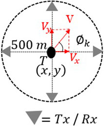
FIGURE 2. Antenna placement.

Moreover, the carrier frequency is f₀ = 10 GHz, the sampling frequency is f_S = 9 MHz, the pulse duration is T_p = 0.56 ms, and the observation time is T_obs = 2.2 ms. The received waveforms are $\mathrm{s}(n{T}_s-{\tau }_{lk})=e^{j2\pi \mathrm{\Delta }{f}_k(n{T}_s-{\tau }_{lk})}$ with frequency increment Δf = 1 MHz between s_k[n] and s_k+1[n] to satisfy the orthogonality assumption and with each waveform energy Es = 1. The signal-to-clutter ratio (SCR) is defined as:

$SCR=\frac{{\sum }_{k=1}^M\Vert {\mathbf{s}}_k{\Vert }^2}{E\left\{{\mathbf{z}}_l^H{\mathbf{z}}_l\right\}}.(48)$

The clutter samples are IID and t-distributed, then $E\left\{{\mathbf{z}}_l^H{\mathbf{z}}_l\right\}=N_s\frac{\nu }{\nu -2}{\sigma }^2$, where $E\left\{|z_l{|}^2\right\}=\frac{\nu }{\nu -2}{\sigma }^2$ is the variance of a complex-t clutter. From the last equation, it is evident that to guarantee a finite positive power, ν > 2.

Following this, we chose the spikier clutter case ν = 2.1. Figures 3 and 4 show the range and Doppler frequency CRLBs of the spikier clutter case for both models I and II, respectively. In addition, we set σ² = 1, and the CRLBs in Figure 4 are shown for spatially correlated clutter.

FIGURE 3

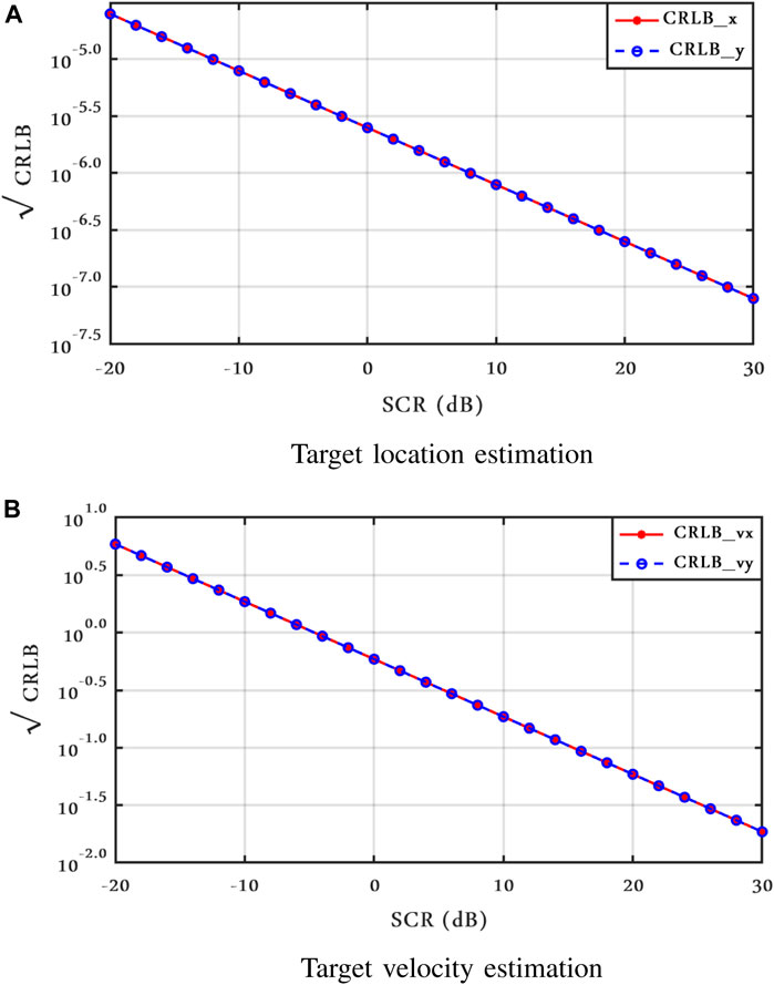
FIGURE 3. CRLB for target location and velocity estimation in Clutter Model I.

FIGURE 4

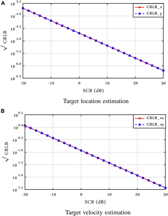
FIGURE 4. CRLB for target location and velocity estimation in Clutter Model II.

Considering (Zhang et al., 2014) the spatially correlated clutter is such that

${\left[\mathbf{\Sigma }\right]}_{p,q}={\sigma }^2{\rho }^{|\left(p-q\right)\mathrm{\Delta }{\alpha }_{p,q}|},(49)$

where ρ is a constant value and we chose ρ = 0.9, and Δα_p,q is the angular distance from the pth receiver to clutter cell and from clutter to the qth receiver.

In the following figures, the joint CRLBs of target location and velocity for different values ν are presented for both clutter cases. We only show CRLB_x and CRLB_vx, since we set the same numerical values for x and y as well as for v_x and v_y; therefore, the CRLBs along the two directions, in this case, are the same.

According to Figure 5, a larger value of ν leads to an increase of the CRLBs in clutter case I. It is worth noting that the clutter power depends on both the scale parameter σ² and the shape parameter ν. In these figures, σ² = 1, then to keep constant the SCR for different values of ν, the energy of the transmitted signals is changed accordingly.

FIGURE 5

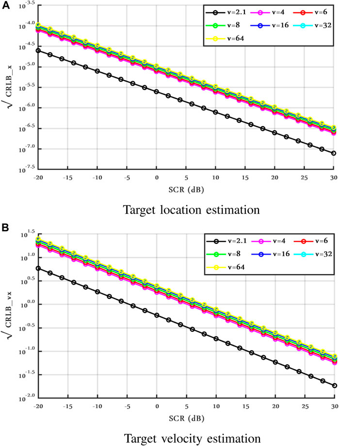
FIGURE 5. CRLBs vs. SCR with different ν, Clutter Model I.

In Figure 6, we plot the CRLBs for the correlated clutter (Model II). In this case, the CRLB tends to increase for lower ν. It is apparent, anyway, that the differences in both models I and II are small with varying values of ν, at least in the tested configuration.

FIGURE 6

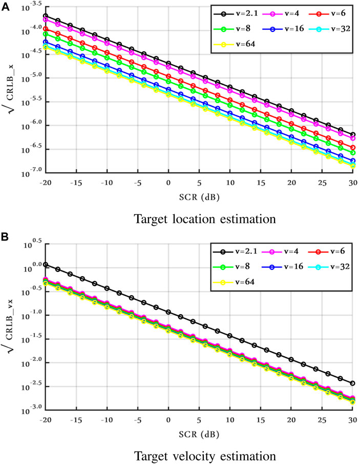
FIGURE 6. CRLBs vs. SCR with different ν, Clutter Model II, ρ = 0.9.

To get a better look at the impact of the parameter ν on the target parameter estimation, under both Model I and Model II, Table 1 provides the CRLBs corresponding to x and v_x at SCR = 0 dB with different values of ν. CRLBs of y and v_y behave quite similarly.

TABLE 1

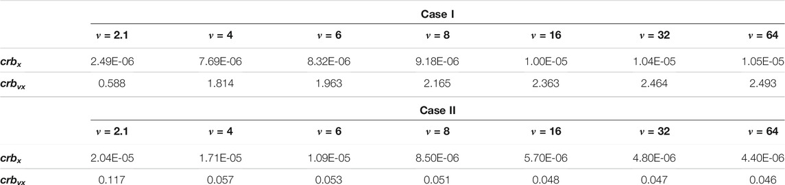
TABLE 1. CRLBs of x and v_x in clutter Model I and Model II with different values of ν, SCR = 0 dB, and ρ = 0.9.

Next, in order to investigate the effect of the correlation coefficient ρ in clutter Model II, Figures 7–9 show the CRLBs as a function of ρ for ν = 2.1 and SCR = 0 dB when the target is still, moving with $vx=10\frac{m}{s}$, $vy=35\frac{m}{s}$, and with $vx=vy=50\frac{m}{s}$, respectively. When the target is still, the CRLBs decrease with increasing values of ρ from −1 to 1, (but ρ has a large impact only when its values are in the interval [0.8; 1]). When the target is moving, the behavior of the CRLBs depends on the value of the target velocity. For some combination of velocity and correlation values, the CRLBs show peaks and notches but the minimum is again reached for ρ = 1. In addition, Figure 10 presents the CRLBs as a function of ρ for ν = 2.1, SCR = 0 dB, and $vx=vy=50\frac{m}{s}$ when the transmitter/receiver antennas are rotated clockwise of 45° with respect to (w.r.t.) the configuration of the previous figures. The CRLBs on the target velocities do not depend strongly on the angular position but the CRLBs on the positions, conversely, do. To better analyze this dependency, keeping fixed the target velocity, (modulus and direction) we rotated counterclockwise the 4 RX/TXs, and in Figures 11–14 we show the CRLBs as a function of the angle between the velocity and the TX/RX on the right (in Figure 2, this angle is equal to −45°), for three values of the correlation coefficient, in the range [−45°: 45°]. Due to the symmetry of the MIMO configuration, these CRLBs are periodic of 90°. These results confirm that for some values of ρ the CRLBs of the target positions strongly depend on the velocity angular direction.

FIGURE 7

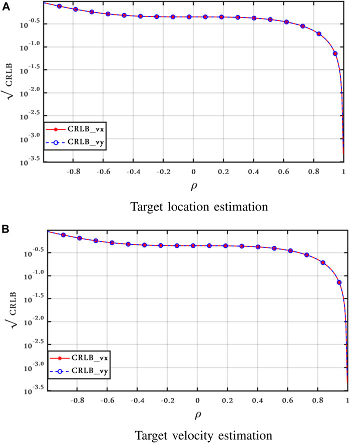
FIGURE 7. CRLBs vs. ρ, Clutter Model II with ν = 2.1, SCR = 0 dB, and v_x = v_y = 0 m/s.

FIGURE 8

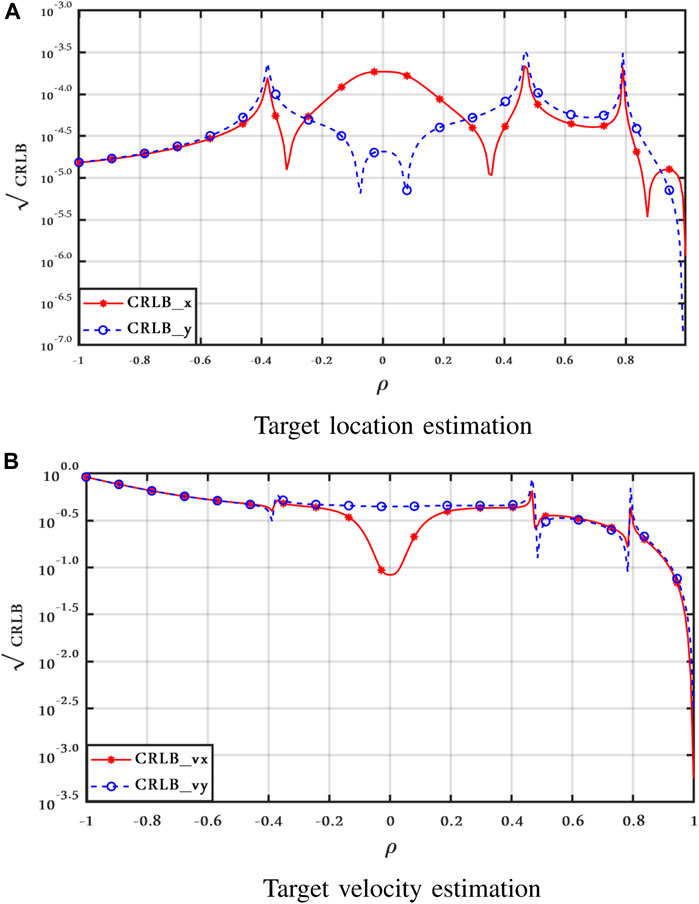
FIGURE 8. CRLBs vs. ρ, Clutter Model II with ν = 2.1, SCR = 0 dB, and v_x = 10, v_y = 35 m/s.

FIGURE 9

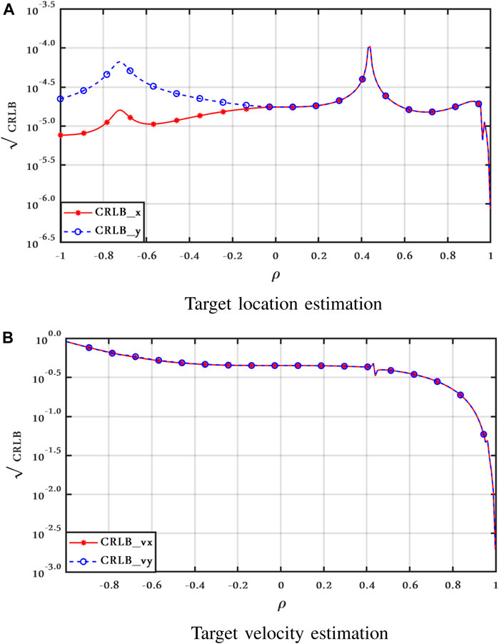
FIGURE 9. CRLBs vs. ρ f, Clutter Model II with ν = 2.1, SCR = 0 dB, and v_x = v_y = 50 m/s.

FIGURE 10

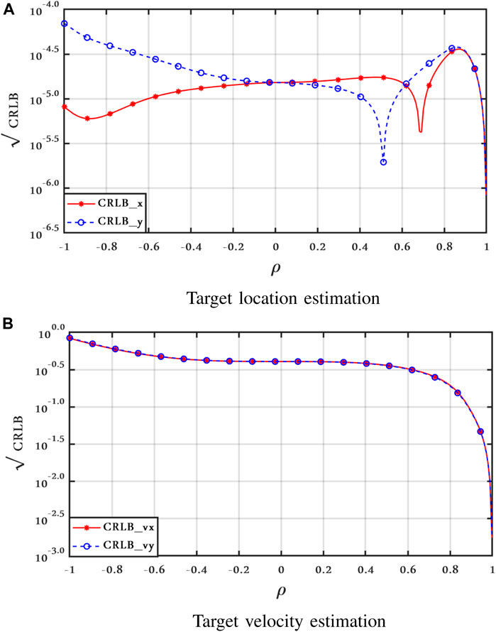
FIGURE 10. CRLBs vs. ρ, Clutter Model II for 45° shifted TX/RX antennas with ν = 2.1, SCR = 0 dB, and v_x = v_y = 50 m/s.

FIGURE 11

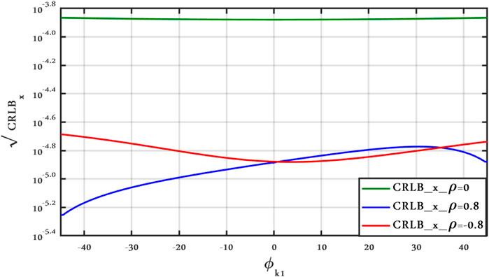
FIGURE 11. CRLB_x vs. ϕ_k1 antenna position, Clutter Model II for different ρ with ν = 2.1, SCR = 0 dB, and v_x = v_y = 50 m/s.

FIGURE 12

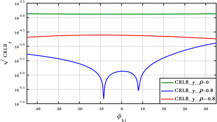
FIGURE 12. CRLB_y vs. ϕ_k1 antenna position, Clutter Model II for different ρ with ν = 2.1, SCR = 0 dB, and v_x = v_y = 50 m/s.

FIGURE 13

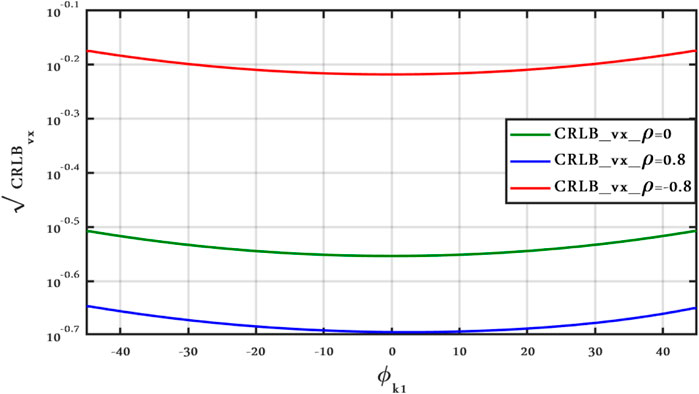
FIGURE 13. CRLB_vx vs. ϕ_k1 antenna position, Clutter Model II for different ρ with ν = 2.1, SCR = 0 dB, and v_x = v_y = 50 m/s.

FIGURE 14

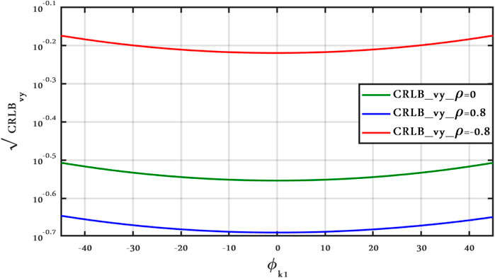
FIGURE 14. CRLB_vy vs. ϕ_k1 antenna position, Clutter Model II for different ρ with ν = 2.1, SCR = 0 dB, and v_x = v_y = 50 m/s.

In Figures 15 and 16, the relation between the bounds and the number of antennas is shown, when the target is located in (0,0). These figures show the effect of increasing the number of sensors in two different scenarios: 1) the radius of the circle is constant, $r=d_l^r=d_k^t=500m$, and the TX/RX antennas are uniformly distributed on the circumference, and 2) the linear distance between each TX/RX antenna pair is fixed to d_m = 49.06 m, and the radius of the circle is variable as a function of the number of antennas M, $r=\frac{d_m}{2\sin (\frac{\pi }{M})}$. As shown in these figures, the performance of the joint target parameter estimation can be remarkably improved by increasing the number of antennas, and this is particularly evident in the second scenario and for the velocity.

FIGURE 15

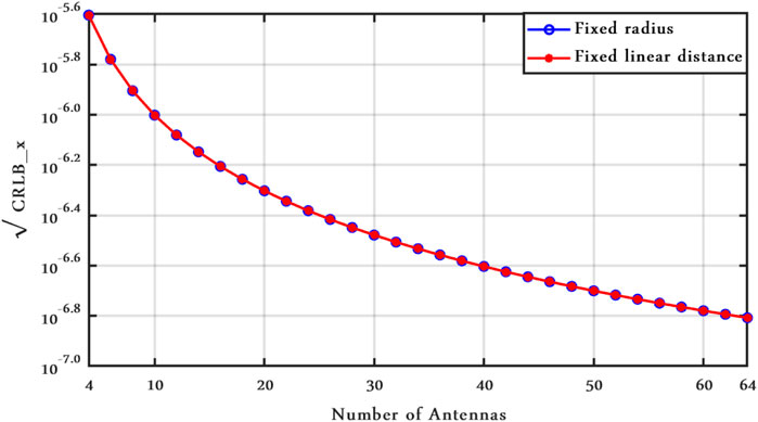
FIGURE 15. CRLB_x vs. number of antenna, Clutter Model I with ν = 2.1, SCR = 0 dB, and v_x = v_y = 50 m/s.

FIGURE 16

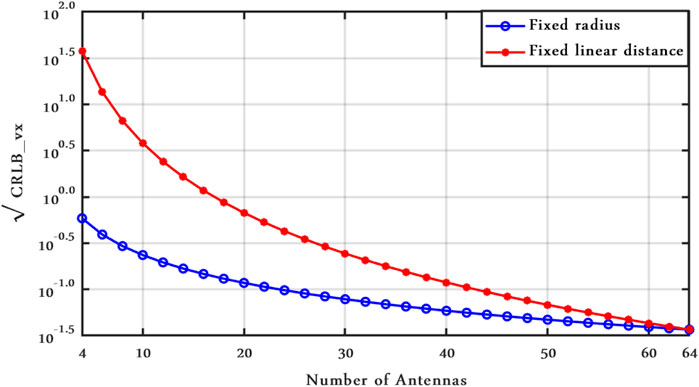
FIGURE 16. CRLB_vx vs. number of antenna, Clutter Model I with ν = 2.1, SCR = 0 dB, and v_x = v_y = 50 m/s.

Additionally, to assess the maximum achievable accuracy of the considered MIMO radar over the area of interest, we define the errors (Maddio et al., 2015; Passafiume et al., 2017; Cidronali et al., 2020) as

$er{r}_{xy}=\sqrt{CRL{B}_x+CRL{B}_y}er{r}_{vxvy}=\sqrt{CRL{B}_{vx}+CRL{B}_{vy}}.(50)$

Figures 17 and 18 illustrate the maximum achievable accuracy (or the error pattern over the area) attained by Eq. 50, in terms of CRLBs in both the clutter models I and II for varying positions with v_x = v_y = 50 m/s, while Figures 19 and 20 show the maximum achievable accuracy for a fixed target. These figures are all calculated for SCR = −15 dB and ν = 2.1.

FIGURE 17

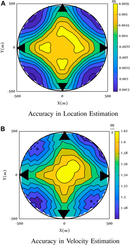
FIGURE 17. Maximum achievable accuracy when the target is moving, Clutter Model I, ν = 2.1 and SCR = −15 dB.

FIGURE 18

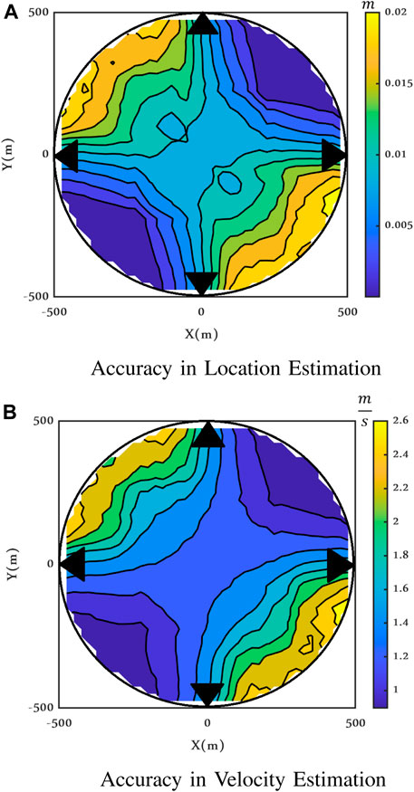
FIGURE 18. Maximum achievable accuracy when the target is moving, Clutter Model II, ρ = 0.9, ν = 2.1, and SCR = −15 dB.

FIGURE 19

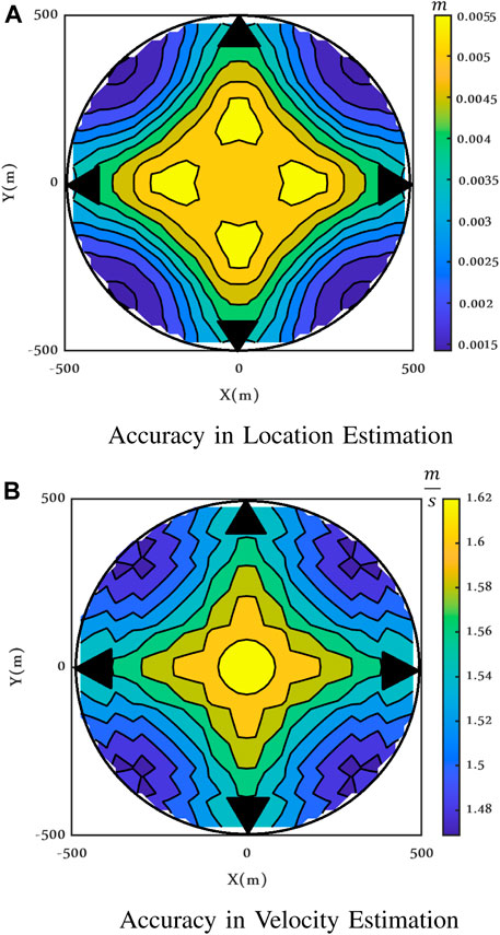
FIGURE 19. Maximum achievable accuracy when the target is still, Clutter Model I, ν = 2.1 and SCR = −15 dB.

FIGURE 20

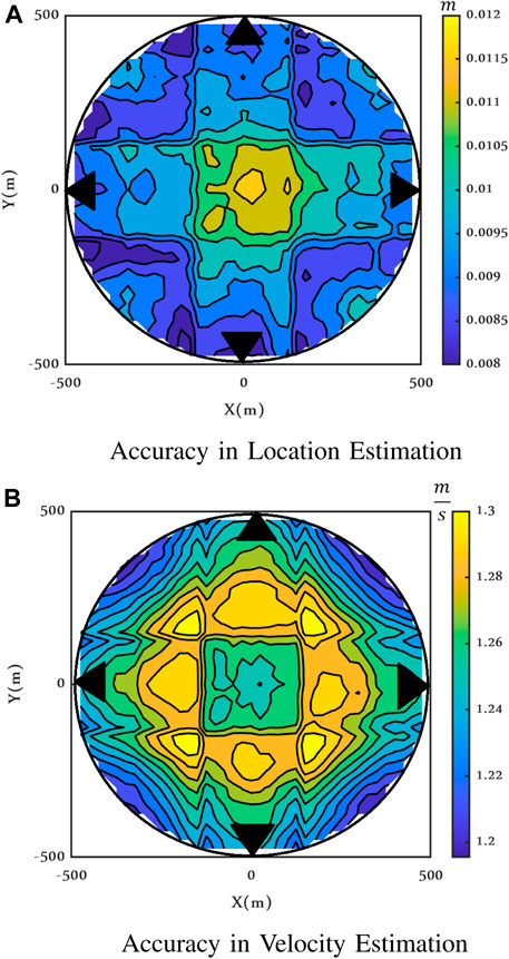
FIGURE 20. Maximum achievable accuracy when the target is still, Clutter Model II, ρ = 0.9, ν = 2.1, and SCR = −15 dB.

Depending on the value of the target velocity along the x and y directions and on the clutter correlation, the shape of the error functioning inside the circle is different, but the range of variations in the considered area is always small, for both range and velocity, for both clutter models I and II.

To check the changes in the CRLBs as a function of the correlation coefficient ρ, in Figure 21, the maximum achievable accuracy is shown for the same scenario described in Figure 18 but for ρ = 0. It is worth observing that ρ = 0 does not mean that the clutter components are independent but only uncorrelated because they are not Gaussian-distributed.

FIGURE 21

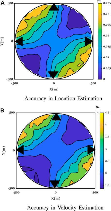
FIGURE 21. Maximum achievable accuracy when the target is moving, Clutter Model II, ρ = 0, ν = 2.1, and SCR = −15 dB.

Finally, to investigate the impact of the position of the transmitters and receivers on the performance of the radar, the error function is shown for a different configuration in Figures 22 and 23, where the receiver antennas are shifted of 45° with respect to the receiver; transmitters and receivers are represented by black and red triangles, respectively. As evident in Figures 22 and 23, configurations with shifted receiver antennas are similar to those of colocated antennas in Figures 17 and 18. The CRLBs are much more affected by the presence of the clutter correlation.

FIGURE 22

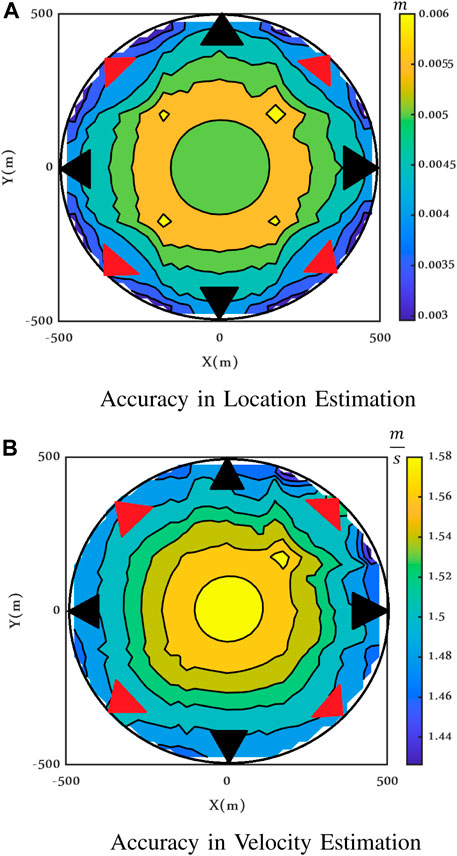
FIGURE 22. Maximum achievable accuracy for shifted receiver antennas when the target is moving, Clutter Model I, ν = 2.1 and SCR = −15 dB.

FIGURE 23

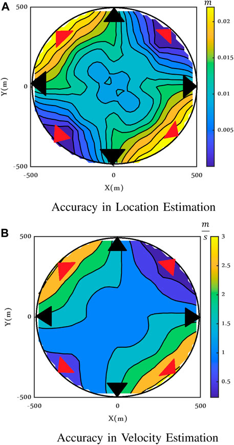
FIGURE 23. Maximum achievable accuracy for shifted receiver antennas when the target is moving, Clutter Model II, ρ = 0, ν = 2.1, and SCR = −15 dB.

6 Conclusion

This article presents the derivation of the CRLBs for the estimation of position and velocity of an isotropic target in a coherent MIMO radar with orthogonally transmitted waveforms in the presence of correlated non-Gaussian clutter, modeled by the complex t-distribution. We derived the CRLBs for two different scenarios: 1) the clutter samples are independent in space and time and 2) the clutter samples are temporally independent but spatially correlated. We then investigated the estimation accuracy as a function of the SCR, the clutter spikiness, and the clutter spatial correlation as well as maximum achievable accuracy in parameter estimation for several radar configurations. The CRLBs show a weak dependency on the spikiness of the clutter but, conversely, a strong dependency on the angular correlation, particularly for the moving target.

Author Disclaimer

The views and conclusions contained are those of the authors and should not be interpreted as necessarily representing the official policies or endorsements, either expressed or implied, of the Air Force Office of Scientific Research or the United States government.

Data Availability Statement

The raw data supporting the conclusion of this article will be made available by the authors, without undue reservation.

Author Contributions

All authors listed have made a substantial, direct, and intellectual contribution to the work and approved it for publication.

Funding

The work of MG and FG has been partially supported by the Italian Ministry of Education and Research (MIUR) in the framework of the CrossLab Project (Departments of Excellence) of the University of Pisa, Laboratory of Industrial Internet of Things (IIoT). This work has been partially funded also by EOARD/AFRL grant FA9550-17-1-0344 on “Exploiting Spatial Diversity in MIMO and Massive MIMO Radar Systems.”

Conflict of Interest

The authors declare that the research was conducted in the absence of any commercial or financial relationships that could be construed as a potential conflict of interest.

Publisher’s Note

All claims expressed in this article are solely those of the authors and do not necessarily represent those of their affiliated organizations, or those of the publisher, the editors, and the reviewers. Any product that may be evaluated in this article, or claim that may be made by its manufacturer, is not guaranteed or endorsed by the publisher.

Supplementary Material

The Supplementary Material for this article can be found online at: https://www.frontiersin.org/articles/10.3389/frsip.2022.822285/full#supplementary-material

References

Brekke, E., Hallingstad, O., and Glattetre, J. (2010). Tracking Small Targets in Heavy-Tailed Clutter Using Amplitude Information. IEEE J. Oceanic Eng. 35 (2), 314–329. doi:10.1109/joe.2010.2044670

CrossRef Full Text | Google Scholar

Cidronali, A., Collodi, G., Lucarelli, M., Maddio, S., Passafiume, M., and Pelosi, G. (2020). Assessment of Anchors Constellation Features in Rssi-Based Indoor Positioning Systems for Smart Environments. Electronics 9 (6), 1026. doi:10.3390/electronics9061026

CrossRef Full Text | Google Scholar

Davis, M. S. (2015). Mimo Radar: Signal Processing, Waveform Design, and Applications to Synthetic Aperture Imaging. Ph.D. dissertation (Atlanta, GA, USA: Georgia Institute of Technology).

Derham, T., Doughty, S., Baker, C., and Woodbridge, K. (2010). Ambiguity Functions for Spatially Coherent and Incoherent Multistatic Radar. IEEE Trans. Aerosp. Electron. Syst. 46 (1), 230–245. doi:10.1109/taes.2010.5417159

CrossRef Full Text | Google Scholar

Farina, A., Gini, F., Greco, M. V., and Verrazzani, L. (1997). High Resolution Sea Clutter Data: Statistical Analysis of Recorded Live Data. IEE Proc. Radar Sonar Navig. 144 (3), 121–130. doi:10.1049/ip-rsn:19971107

CrossRef Full Text | Google Scholar

Fishler, E., Haimovich, A., Blum, R., Chizhik, D., Cimini, L., and Valenzuela, R. (2004). “Mimo Radar: An Idea Whose Time Has Come,” in Proceedings of the 2004 IEEE Radar Conference (IEEE Cat. No. 04CH37509) (Philadelphia, PA, USA: IEEE), 71–78.

Google Scholar

Fishler, E., Haimovich, A., Blum, R. S., Cimini, L. J., Chizhik, D., and Valenzuela, R. A. (2006). Spatial Diversity in Radars-Models and Detection Performance. IEEE Trans. Signal. Process. 54 (3), 823–838. doi:10.1109/tsp.2005.862813

CrossRef Full Text | Google Scholar

Fortunati, S., Farina, A., Gini, F., Graziano, A., Greco, M. S., and Giompapa, S. (2010). Least Squares Estimation and Cramér-Rao Type Lower Bounds for Relative Sensor Registration Process. IEEE Trans. Signal Process. 59 (3), 1075–1087.

Google Scholar

Fortunati, S., Gini, F., Greco, M. S., Zoubir, A. M., and Rangaswamy, M. (2019). Semiparametric Crb and Slepian-Bangs Formulas for Complex Elliptically Symmetric Distributions. IEEE Trans. Signal. Process. 67 (20), 5352–5364. doi:10.1109/tsp.2019.2939084

CrossRef Full Text | Google Scholar

Fortunati, S., Gini, F., Greco, M. S., Zoubir, A. M., and Rangaswamy, M. (2018). Semiparametric Inference and Lower Bounds for Real Elliptically Symmetric Distributions. IEEE Trans. Signal Process. 67 (1), 164–177.

Google Scholar

Gini, F. (1998). A Radar Application of a Modified Cramer-Rao Bound: Parameter Estimation in Non-gaussian Clutter. IEEE Trans. Signal. Process. 46 (7), 1945–1953. doi:10.1109/78.700966

CrossRef Full Text | Google Scholar

Gini, F., and Greco, M. V. (1999). Suboptimum Approach to Adaptive Coherent Radar Detection in Compound-Gaussian Clutter. IEEE Trans. Aerosp. Electron. Syst. 35 (3), 1095–1104. doi:10.1109/7.784077

CrossRef Full Text | Google Scholar

Gini, F., and Reggiannini, R. (2000). On the Use of Cramer-rao-like Bounds in the Presence of Random Nuisance Parameters. IEEE Trans. Commun. 48 (12), 2120–2126. doi:10.1109/26.891222

CrossRef Full Text | Google Scholar

Godrich, H., Haimovich, A. M., and Blum, R. S. (2008). “Cramer Rao Bound on Target Localization Estimation in Mimo Radar Systems,” in 2008 42nd Annual Conference on Information Sciences and Systems (Princeton, NJ, USA: IEEE), 134–139. doi:10.1109/ciss.2008.4558509

CrossRef Full Text | Google Scholar

Godrich, H., Haimovich, A. M., and Blum, R. S. (2008). “Target Localization Accuracy and Multiple Target Localization: Tradeoff in Mimo Radars,” in 2008 42nd Asilomar Conference on Signals, Systems and Computers (Pacific Grove, CA, USA: IEEE), 614–618. doi:10.1109/acssc.2008.5074479

CrossRef Full Text | Google Scholar

Godrich, H., Haimovich, A. M., and Blum, R. S. (2010). Target Localization Accuracy Gain in Mimo Radar-Based Systems. IEEE Trans. Inform. Theor. 56 (6), 2783–2803. doi:10.1109/tit.2010.2046246

CrossRef Full Text | Google Scholar

Goodman, N. R. (1963). Statistical Analysis Based on a Certain Multivariate Complex Gaussian Distribution (An Introduction). Ann. Math. Statist. 34 (1), 152–177. doi:10.1214/aoms/1177704250

CrossRef Full Text | Google Scholar

Haimovich, A. M., Blum, R. S., and Cimini, L. J. (2007). Mimo Radar with Widely Separated Antennas. IEEE Signal. Process. Mag. 25 (1), 116–129.

Google Scholar

Hassanien, A., Vorobyov, S. A., and Gershman, A. B. (2012). Moving Target Parameters Estimation in Noncoherent Mimo Radar Systems. IEEE Trans. Signal. Process. 60 (5), 2354–2361. doi:10.1109/tsp.2012.2187290

CrossRef Full Text | Google Scholar

He, Q., Blum, R. S., Godrich, H., and Haimovich, A. M. (2008). “Cramer-rao Bound for Target Velocity Estimation in Mimo Radar with Widely Separated Antennas,” in 2008 42nd Annual Conference on Information Sciences and Systems (Princeton, NJ, USA: IEEE), 123–127. doi:10.1109/ciss.2008.4558507

CrossRef Full Text | Google Scholar

He, Q., Blum, R. S., Godrich, H., and Haimovich, A. M. (2010). Target Velocity Estimation and Antenna Placement for Mimo Radar with Widely Separated Antennas. IEEE J. Sel. Top. Signal. Process. 4 (1), 79–100. doi:10.1109/jstsp.2009.2038974

CrossRef Full Text | Google Scholar

He, Q., Blum, R. S., and Haimovich, A. M. (2010). Noncoherent Mimo Radar for Location and Velocity Estimation: More Antennas Means Better Performance. IEEE Trans. Signal. Process. 58 (7), 3661–3680. doi:10.1109/tsp.2010.2044613

CrossRef Full Text | Google Scholar

Krishnaiah, P. R., and Lin, J. (1986). Complex Elliptically Symmetric Distributions. Commun. Stat. - Theor. Methods 15 (12), 3693–3718. doi:10.1080/03610928608829341

CrossRef Full Text | Google Scholar

Li, J., and Stoica, P. (2009). Concepts and Applications of a Mimo Radar System with Widely Separated Antennas. Hoboken, NJ, USA: Wiley-IEEE Press.

Google Scholar

Li, J., and Stoica, P. (2008). MIMO Radar Signal Processing. Hoboken, NJ, USA: John Wiley & Sons.

Google Scholar

Li, J., and Stoica, P. (2007). Mimo Radar with Colocated Antennas. IEEE Signal. Process. Mag. 24 (5), 106–114. doi:10.1109/msp.2007.904812

CrossRef Full Text | Google Scholar

Maddio, S., Passafiume, M., Cidronali, A., and Manes, G. (2015). “A Distributed Positioning System Based on Real-Time Rssi Enabling Decimetric Precision in Unmodified Ieee 802.11 Networks,” in 2015 IEEE MTT-S International Microwave Symposium (Phoenix, AZ, USA: IEEE), 1–4. doi:10.1109/mwsym.2015.7166926

CrossRef Full Text | Google Scholar

Min, J., Niu, R., and Blum, R. (2011). Bayesian Target Location and Velocity Estimation for Multiple-Input Multiple-Output Radar [j]. IET Radar, Sensor and Navigation 5 (6), 666–670.

Google Scholar

Novey, M., Adali, T., and Roy, A. (2009). A Complex Generalized Gaussian Distributionâcharacterization, Generation, and Estimation. IEEE Trans. Signal Process. 58 (3), 1427–1433.

Google Scholar

Ollila, E., Tyler, D. E., Koivunen, V., and Poor, H. V. (2012). Complex Elliptically Symmetric Distributions: Survey, New Results and Applications. IEEE Trans. Signal. Process. 60 (11), 5597–5625. doi:10.1109/tsp.2012.2212433

CrossRef Full Text | Google Scholar

Passafiume, M., Maddio, S., and Cidronali, A. (2017). An Improved Approach for RSSI-Based Only Calibration-free Real-Time Indoor Localization on IEEE 802.11 and 802.15.4 Wireless Networks. Sensors 17 (4), 717. doi:10.3390/s17040717

PubMed Abstract | CrossRef Full Text | Google Scholar

Peilin Sun, P., Tang, J., and Shuang Wan, S. (2014). Cramer-rao Bound of Joint Estimation of Target Location and Velocity for Coherent Mimo Radar. J. Syst. Eng. Electron. 25 (4), 566–572. doi:10.1109/jsee.2014.00066

CrossRef Full Text | Google Scholar

Raninen, E., Ollila, E., and Tyler, D. (2021). On the Variability of the Sample Covariance Matrix under Complex Elliptical Distributions. IEEE Signal. Process. Lett. 28, 2092–2096. doi:10.1109/lsp.2021.3117443

CrossRef Full Text | Google Scholar

Sangston, K. J., Gini, F., and Greco, M. S. (2012). Coherent Radar Target Detection in Heavy-Tailed Compound-Gaussian Clutter. IEEE Trans. Aerosp. Electron. Syst. 48 (1), 64–77. doi:10.1109/taes.2012.6129621

CrossRef Full Text | Google Scholar

Sangston, K. J., Gini, F., Greco, M. V., and Farina, A. (1999). Structures for Radar Detection in Compound Gaussian Clutter. IEEE Trans. Aerosp. Electron. Syst. 35 (2), 445–458. doi:10.1109/7.766928

CrossRef Full Text | Google Scholar

Stoica, P., and Nehorai, A. (1990). Music, Maximum Likelihood, and Cramer-Rao Bound: Further Results and Comparisons. IEEE Trans. Acoust. Speech, Signal. Process. 38 (12), 2140–2150. doi:10.1109/29.61541

CrossRef Full Text | Google Scholar

Tajer, A., Jajamovich, G. H., Wang, X., and Moustakides, G. V. (2010). Optimal Joint Target Detection and Parameter Estimation by Mimo Radar. IEEE J. Sel. Top. Signal. Process. 4 (1), 127–145. doi:10.1109/jstsp.2010.2040104

CrossRef Full Text | Google Scholar

Zhang, X., El Korso, M. N., and Pesavento, M. (2014). “Mimo Radar Performance Analysis under K-Distributed Clutter,” in 2014 IEEE International Conference on Acoustics, Speech and Signal Processing (ICASSP) (Florence, Italy: IEEE), 5287–5291. doi:10.1109/icassp.2014.6854612

CrossRef Full Text | Google Scholar

Zhang, X., El Korso, M. N., and Pesavento, M. (2017). Mimo Radar Target Localization and Performance Evaluation under Sirp Clutter. Signal. Process. 130, 217–232. doi:10.1016/j.sigpro.2016.06.031

CrossRef Full Text | Google Scholar