 Simeon Mayala1*
 Ida Herdlevær2,3
 Jonas Bull Haugsøen2,3
 Shamundeeswari Anandan2,3
 Sonia Gavasso2,3
 Morten Brun1
- 1Department of Mathematics, University of Bergen, Bergen, Norway
- 2Department of Clinical Medicine, University of Bergen, Bergen, Norway
- 3Neuro-SysMed, Department of Neurology, Haukeland University Hospital, Bergen, Norway
In this paper, we propose a minimum spanning tree-based method for segmenting brain tumors. The proposed method performs interactive segmentation based on the minimum spanning tree without tuning parameters. The steps involve preprocessing, making a graph, constructing a minimum spanning tree, and a newly implemented way of interactively segmenting the region of interest. In the preprocessing step, a Gaussian filter is applied to 2D images to remove the noise. Then, the pixel neighbor graph is weighted by intensity differences and the corresponding minimum spanning tree is constructed. The image is loaded in an interactive window for segmenting the tumor. The region of interest and the background are selected by clicking to split the minimum spanning tree into two trees. One of these trees represents the region of interest and the other represents the background. Finally, the segmentation given by the two trees is visualized. The proposed method was tested by segmenting two different 2D brain T1-weighted magnetic resonance image data sets. The comparison between our results and the gold standard segmentation confirmed the validity of the minimum spanning tree approach. The proposed method is simple to implement and the results indicate that it is accurate and efficient.
1 Introduction
A brain tumor is a collection of abnormal cells in the brain: they may be malignant (cancerous) or benign (noncancerous) and can be categorized as primary or secondary. Primary brain tumors originate in the brain and are either glial or non-glial. Glial brain tumors are the most common, arising from the supporting cells of the brain. Non-glial tumors may originate from any other tissue in the brain, such as meninges, neurons, blood vessels, and glands. Primary tumors can be malignant (cancerous) or benign. Secondary brain tumors develop in another part of the body and metastasize to the brain. Cancers that commonly metastasize to the brain include lung cancer, breast cancer, kidney cancer, and skin cancer. Secondary brain tumors are always malignant. Brain tumors may be located in any part of the brain. Magnetic resonance imaging (MRI) is important in diagnosing and monitoring brain tumors. Brain tumor segmentation is an essential step in analyzing and interpreting such images (Ciesielski and Udupa, 2011; Banerjee et al., 2016). Segmenting brain tumors using automatic techniques is challenging because of factors that cause complexity during segmentation. These factors include the location in the brain, irregular shapes, different sizes, types of tumors, blurred boundaries, and noise.
The problem of brain tumor segmentation is studied in different research works. Skull- stripping is a fundamental preprocessing step to isolate the brain tissue before brain tumor segmentation (Kalavathi and Prasath, 2016). It removes the non-brain tissues such as skin, fat, muscle, neck, and eyeballs from the image. This step simplifies the complexity of the brain image and increases the speed and accuracy of the segmentation process. Some popular tools developed for skull stripping include: Freesurfer’s strip skull (FSS) (Dale et al., 1999), Brain Surface Extractor (BSE) (Roy and Maji, 2015), Brain Extraction Tool (BET) (Smith, 2000), Hybrid Approach (HWA) (Ségonne et al., 2004), Robust Brain Extraction (ROBEX) (Iglesias et al., 2011) and Hahn and Peitgen’s Watershed Algorithm (WAT) (Hahn and Peitgen, 2000).
Different methods are used for brain tumor segmentation. They are categorized based on their formulation and how they perform the segmentation. These include traditional image segmentation, machine learning, deep learning (Huang et al., 2021), and graph-based methods such as those based on the minimum spanning tree (MST) (Long and Sun 2020; Kang 2021). The limited flexibility of many existing segmentation methods, especially those reviewed below, necessitates careful fine-tuning of parameters. In many works, an MST is used for segmenting images with control parameters such as specifying thresholds, specifying the size of the regions to be segmented and the number of neighbors to be considered. We propose a method that uses the MST without tuning parameters except a smoothing parameter used in the preprocessing step. Moreover, our method segments brain tumors without the necessity of skull stripping. Concerning what is stated in the article Apropos of Signal Processing (Nandi, 2021), we adopt the existing theoretical ideas and algorithms and use them to segment brain tumors.
Before describing the proposed method, we review related literature to show how the MST is applied in image segmentation. Zahn (1971) proposed an MST-based approach for addressing the problem of detecting and separating different inherent clusters. Zahn’s method was aimed at clustering of point clouds and segmenting images. The method obtains segments by dropping inconsistent edges, with weights below the threshold, to break the minimum spanning tree into a collection of trees. This idea is a powerful tool for point clustering and image segmentation. However, depending on the chosen threshold, the high variability regions are likely to be split into multiple regions that should be merged. To address the shortcoming, Urquhart (1982) proposed a non-parametric hierarchic clustering method based on the concept of limited neighborhood sets and Gabriel graph.
Xu and Uberbacher (1997) proposed another method for image segmentation based on the MST. The method constructs a weighted planar graph from a 2D gray-level image. Then, the MST is constructed from the graph so that the connected homogeneous regions correspond to one sub-tree of the spanning tree. The algorithm partitions the tree into a set of subtrees and each subtree consists of the nodes with similar gray levels. To avoid forming many small regions, conditions are introduced. Partitions are controlled by the condition that each partitioned region has at least a specified number of pixels and that two adjacent regions have average gray levels that differ by more than a specified value.
Felzenszwalb and Huttenlocher (2004) proposed a graph-based method for image segmentation. The method defines a predicate for measuring the evidence for a boundary between two regions in the image. Based on the defined predicate, an efficient segmentation algorithm is developed. It considers two quantities to measure the evidence for the boundary. The paper defines two criteria whether there is evidence for a boundary between components or partitions. The two criteria include the internal difference (the largest weight in the MST of the component) and the difference between the two components. A special property of the algorithm is its ability to preserve details in “low variability regions while ignoring details in high variability regions.” The algorithm segments the images efficiently and produces segments that capture the global properties.
Other researchers improved a successful data clustering method based on Prim’s MST representation for performing image segmentation (Saglam and Baykan, 2017). The algorithm scans the complete MST structure of the entire image to obtain and cut the inconsistent edges. Also, they develop a cutting criterion that considers several local and global features. The proposed method competes with other algorithms in terms of execution time. Also, Long and Sun (2020) proposed an algorithm to tackle the challenge of the ill-posedness of image segmentation. The proposed algorithm is based on the MST. They propose a different formula for RGB color space with respect to angular distance color as the weight of judge standard of the segmentation. The judging standard involves the spatial distance and vector relationship between two pixels. The experimental results show that the proposed algorithm is effective.
In summary, our focus is to segment brain tumors without skull stripping from the T1-weighted MRI and compare the result to their ground truth segmentation. We utilize the MST efficiency to extract the brain tumor directly without skull stripping. Also, we test the method by segmenting the brain on simulated MRI for the brain and compare the result to the ground truth. The proposed method is mainly composed of the following steps: (I) making a graph and constructing a minimum spanning tree and (II) interactively segmenting the region of interest.
2 Materials and Methods
2.1 Material
In this paper, we use two different image data sets. The first data set includes 3,064 slices of 2D brain T1-weighed (T1W) contrast-enhanced (CE)-MRI from 233 patients collected at Nanfang Hospital, Guangzhou, China, and General Hospital, Tianjin Medical University, China. The images are classified into three types of brain tumors, labeled as follows: 1) meningioma, 2) glioma, and 3) pituitary tumors (Cheng et al., 2015; Cheng et al., 2016). The images were acquired with a slice thickness of 6 mm and the slice gap is 1 mm. The image dataset is provided in the Matlab format (.mat). Each file stores a struct containing different fields for an image. The fields included in each file are labels for the tumor type, an anonymized patient ID, the image data, tumor borders, and tumor masks. The reader is referred to (Cheng, 2017) for additional images and original images.
The second data sets consist of 20 simulated T1W MR images of normal brains from the BrainWeb website. They are anatomical models consisting of a set of 3D tissue membership volumes, one for each tissue class: background, cerebrospinal fluid (CSF), gray Matter, white matter, fat, muscle, muscle/skin, skull, vessels, around fat, dura mater, bone marrow. Each label at a voxel in the anatomical model represents the tissue that contributes the most to that voxel. They have a 0.5 mm isotropic voxel size and they are stored in the MINC format. For more information refer to Cocosco et al. (1997) and Aubert-Broche et al. (2006).
2.2 Methods
In this section, we establish a segmentation method based on the MST. We define important terms that will be referred to when using the proposed method.
2.2.1 Graph
Let G = (V, E) be connected, undirected and weighted graph with nodes V = {v1, v2, v3, … , vn} and edges E = {e1, e2, e3, … , em} such that ei is a weighted link between two neighboring nodes, and |V| = n, |E| = m. The graph is obtained after mapping an image into a graph, and each node in the graph G represents a pixel in the input image. If the pixel’s intensity value of the image at position (x, y) is represented by Ix,y, then, the corresponding node’s value is
The associated weight wj to the edge ej is a measure of the similarity between two neighboring pixels. The edge’s weight is the absolute value of the difference between the intensity values of the pixels vi and
Note that vi and
2.2.2 Path in a Graph
A path P in graph G is a sequence of edges joining two terminal nodes say P = {vi, … , vk} where vi and vk are the terminal nodes in the path. It is a non-empty subgraph or graph consisting of nodes in the form of
where V* ⊆ V and E* ⊆ E. Since a path is a natural seguence of its vertices then vi, … , vk and vk, … , vi denote the same thing (Diestel, 2000). Since we are considering a connected graph then, there exist at least one path between any two pairs of nodes in the graph.
2.2.3 Tree and Spanning Tree in a Graph G
A tree T is a connected graph without any cycle. A tree with n nodes has n − 1 edges. For any two nodes in the tree T there exist a unique path P linking the two nodes. Since a tree is minimally connected then for every edge e ∈ T, T − e is disconnected. Also, for any two non-adjacent vertices vi, vk ∈ T, T plus the edge connecting vi and vk is cyclic because T is maximally acyclic (Diestel, 2000). The spanning tree of the connected graph G is a tree in G which contains all nodes of G. Note that a graph can have many spanning trees.
2.2.4 Minimum Spanning Tree of a Graph G
A minimum spanning tree of a graph G is a spanning tree whose weight is minimum among all spanning trees of the graph G. It is the shortest spanning tree with the least total weight of all edges among all possible spanning trees of the graph G (Morris et al., 1986). Assuming that wi is the weight associated with the edge ei in E, we can define an MST to be T = (V, E′), E′ ⊆ E such that
2.2.5 Segmentation Criteria
Pixels within the region of interest (ROI) have relatively similar intensity values, so the edges connecting nodes in the ROI have relatively small weights differences. Likewise, pixels in the background have relatively similar intensity values, so the edges connecting nodes in the background have relatively small weights differences. Then, a higher difference is expected at the boundary of the ROI and the background. We use this fact to establish that there is a boundary between the ROI and the background.
Let R1 and R2 be regions each containing several vertices in the MST. Let vi and vj be vertices in the regions R1 and R2, respectively. The boundary between R1 and R2 is defined by the edge with the maximum weight in the path P connecting vi ∈ R1 and vj ∈ R2. Then, the segmentation criterion is
where, Bd (R1, R2) represents the boundary between regions R1 and R2, w (ek) is the weight of edge ek. We implement the segmentation method and produce results by considering three situations. The first situation is when the regions R1 and R2 are loosely connected (the boundary is clear). The second situation is when regions R1 and R2 are connected (the boundary is not clear but it exists). The third situation is when the regions R1 and R2 are strongly connected (there is no boundary).
2.3 Implementation Steps
2.3.1 Construction of Minimum Spanning Tree
The input image is preprocessed by applying a Gaussian filter to reduce or remove artifacts because it is important to reduce the influence of noise in the computed edges’ weights. Edges of the graph are computed together with corresponding weights in which each vertex represents a pixel from the image. The weight of each edge is computed by taking the absolute difference of two neighboring nodes. We construct a sparse graph from which an MST is constructed. We use Scipy package (Virtanen et al., 2020) to compute both the graph and its MST. The Kruskal algorithm is used for computing the MST.
2.3.2 Interactive Part
Vertices Identification
The ROI is identified by visual inspection. Then a node is selected from the ROI and another from the background. To simplify this step, we create a graphical user interface for selecting nodes by clicking. Also, we create a reference image for storing the vertices in their respective positions. We bind the reference image behind the input image so that when a pixel is clicked on the input image the pixel coordinate extracts a node in the reference image. To identify the nodes, click once inside the ROI and then the background. For efficiency, the point selected as background should be close to the ROI. We use a Python standard graphical user interface package, Tkinter for creating the interactive window (Lundh, 1999).
Separating the ROI and the Background
The identified vertices are used for generating a path from the MST. We use the breadth-first search tree to find the path from the MST. We use Scipy package to extract the path in the MST connecting the two vertices (Virtanen et al., 2020). We run a script (only on the path) to search and identify the edge with the maximum weight and remove it from the MST. This step updates the MST by splitting it into subtrees. The updated MST is mapped back to the image to visualize the final segmentation. The steps in the interactive part can be performed repeatedly to separate more regions of interest and the MST will continue updating. The steps are summarized in Figure 1.
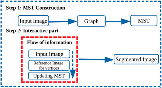
FIGURE 1. The schematic flow diagram shows the steps involved in the segmentation process. Step 1: The image is filtered using a Gaussian filter and then weights are computed for the pixel neighbor graph. Then, the minimum spanning tree (MST) is constructed from the graph. Step 2: The region of interest (ROI) is segmented interactively. The ROI and the background are selected by clicking. Then, the MST is updated to separate the ROI from the background. New labels are assigned and reshaped back to the shape of the input image. The reshaped labels are visualized to show the segmented ROI from the background.
3 Results
3.1 Steps of Segmenting the Region of Interest
We used the MST approach to interactively segment brain tumors from different brain regions (Figure 2). The first data set provided in . mat files was converted into .jpg format. The images were preprocessed using sigma = 0.1, except for a few images that needed a higher value. For the interactive part, the image was converted using Python Imaging Library (PIL) to give it a format compatible with Tkinter (Umesh, 2012). The interactive window was used to select the ROI and background (Figures 2B,C), which resulted in tumor segmentation (Figure 2D).
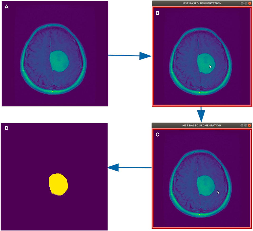
FIGURE 2. Steps for segmenting a brain tumor. (A) Representative axial MRI section of a brain with a tumor giving a higher intensity signal. (B,C) Interactive window showing a cursor selecting a pixel inside and outside the tumor, respectively. (D) Final segmented tumor.
3.2 Segmentation Results: Region of Interest is Well Separated From the Background
Images from the first data set were used to evaluate the MST approach when segmenting ROIs loosely connected to the background (Figure 3). We followed the steps described in (Figure 2) to segment the brain tumors. In the instances/cases where the ROIs are loosely connected to the background, a sigma value of 0.1 is used in the preprocessing step to obtain the segmentation.
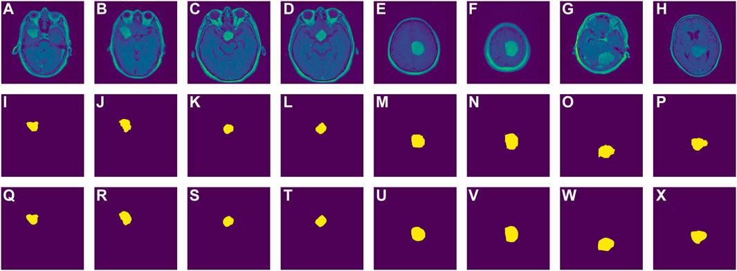
FIGURE 3. Brain tumor segmentation of images from the first data set using minimum spanning tree. (A–H) Representative axial MRI sections of brains with tumors giving a higher intensity signal. (I–P) Segmented images (A–H) using minimum spanning tree. (Q–X) Ground truth images.
Figure 4 presents segmentation results obtained after segmenting MRI brain images without tumors. The images are from T1W simulated brain MRI volume. They are axial T1-weighted MRI images filtered by tuning a sigma = 0.3. To segment the brain from each image we undergo the same steps as described in (Figure 2) but in this case, we select the brain as the ROI and the skull as the background.
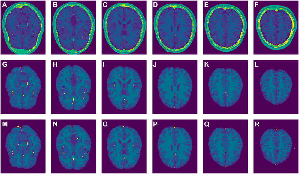
FIGURE 4. Brain segmentation of images from the second data set using the minimum spanning tree. (A-F) Representative axial MRI sections of brains. (G–L) Segmented images (A–F) using the minimum spanning tree. (M–R) Ground truth images: obtained from the labels representing cerebrospinal fluid, gray matter, white matter and vessels.
3.3 Segmentation Results: Region of Interest is Not Well Separated From the Background
The tumor’s location in the brain is one of the obstacles that hinder the segmentation process. Filtering can improve the boundary between the tumor and the neighboring tissues. Figure 5 presents results for the tumor segmented by tuning different values of sigma.
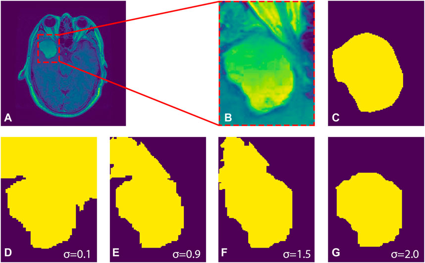
FIGURE 5. Effect of filtering on the segmented region of interest. (A) Representative axial MRI section of a brain with a tumor giving a higher intensity signal. (B) The zoomed-in part of the image from (A). (C) Ground truth image. (D–G) Segmented image when sigma is 0.1, 0.9, 1.5, and 2.0, respectively.
Figure 6 shows how the input image in Figure 5 can be efficiently segmented by using the proposed method without tuning different values of sigma. The image is filtered by using sigma = 0.1 and then the brain tumor is segmented interactively without changing values of sigma.
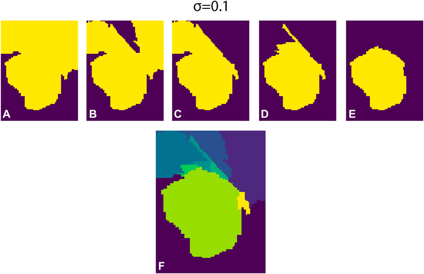
FIGURE 6. Segmenting the tumor interactively without tuning parameters. (A–E) Segmenting the brain tumor interactively when sigma = 0.1. (F) Visualized labels of the segmented tumor and the background.
Another example of segmenting a tumor interactively without tuning different values of sigma is presented in Figure 7.
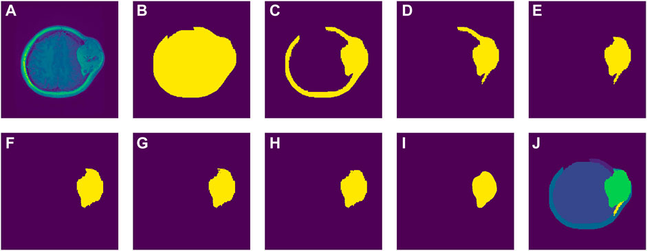
FIGURE 7. Segmenting a brain tumor that is strongly connected to the skull. (A) Representative axial MRI section of a brain with a tumor giving a higher intensity signal. (B–G) Segmenting the brain tumor interactively sigma = 0.9. (H) Segmented image using minimum spanning tree. (I) Ground truth. (J) Visualized labels of the segmented tumor and the background.
3.4 Performance Analysis
We use the Jaccard Index, Dice similarity Coefficient, Sensitivity, and Specificity of the binary label to evaluate the method’s performance. Let L be the set of labels in the MRI 2D slice. We classify them into labels representing the object of interest and the background. We binarize the set of labels into two unique labels such that
Let LT be the binarized labels in a ground truth brain tumor mask and LP be the binarized labels in a predicted brain tumor segmented using the MST approach. We can also use the concept of true positive (TP), false positive (FP), true negative (TN) and false-negative (FN) to check the performance of the method. TP represents the labels that are correctly classified as brain tumor. FP represents the labels that are incorrectly classified as brain tumor. They are not in the tumor region but classified as being in a brain tumor region. TN are labels that are correctly classified as non-tumor material, FN represents the labels that are incorrectly classified as non-tumor materials (they are tumor region labels but classified as being in a non-tumor region). The concept is paraphrased from Hua et al. (2020). The Jaccard Index (JI) is given by
The Dice Similarity Coefficient (Wang et al., 2019) is computed by using
We define |LT (x, y) ∩ LP (x, y)| to be the number of similar labels appearing at similar positions (x, y) in both LT and LP. |LT (x, y)| is the number of labels at (x, y) positions in the ground truth labels and |LP (x, y)| is the number of labels at (x, y) positions in the predicted labels. |LT (x, y) ∪ LP (x, y)| represents the number of labels which are in LP or in LT or in both.
We also compute the sensitivity and specificity which show the percentage of brain tumor and non-brain tumor voxels recognized respectively
We present the quantitative measurement of the segmentation accuracy by comparing the results obtained using the MST-based approach to the ground truth. We compute the Jaccard Indices, Dice Similarity coefficients, Sensitivity, and Specificity. The Jaccard indices and Dice Similarity metrics range from zero to one. A value zero means there is no overlap between the segmented region using the proposed method and the ground truth. The value 1 means there is a perfect overlap between ground truth segmentation and the one obtained using the proposed method.
We randomly sampled 300 slices from the first data set and segmented them using the proposed method and compared to the results in a preprint by Kasar et al. (2021) in Table 2.
Figures 8, 9 present graphs for representative images showing how filtering can affect the final segmentation. We use Jaccard indices, Dice similarity coefficients, sensitivity, and specificity as measures of similarity of the segmented ROI to the ground truth. Looking at the range of sigma in relation to the measure of similarity, it indicates that for images whose ROI is well separated from the background a value of sigma close to zero provides satisfactory results with a single click. For images whose ROI is not well separated from the background it can be challenging to obtain acceptable results because it may require additional interactive steps (see Figures 8, 9).
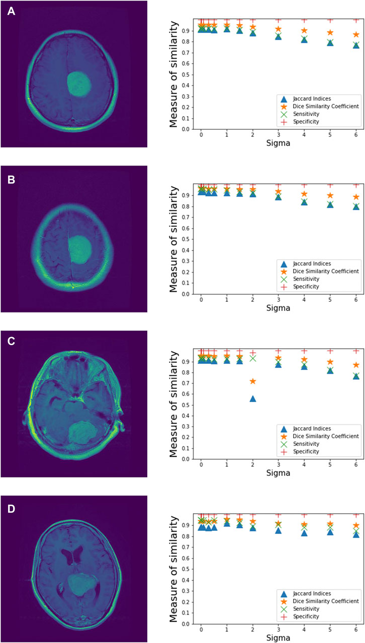
FIGURE 8. Influence of sigma on the performance of the minimum spanning tree-based method. (A–D) Images and the corresponding graphs showing measures of similarity (vertical axis) of the segmented images using the minimum spanning tree method in relation to the tuned sigma (horizontal axis). The sigma values tested include: 0, 0.01, 0.1, 0.3, 0.5, 1.0, 1.5, 2.0, 3.0, 4.0, 5.0, and 6.0.
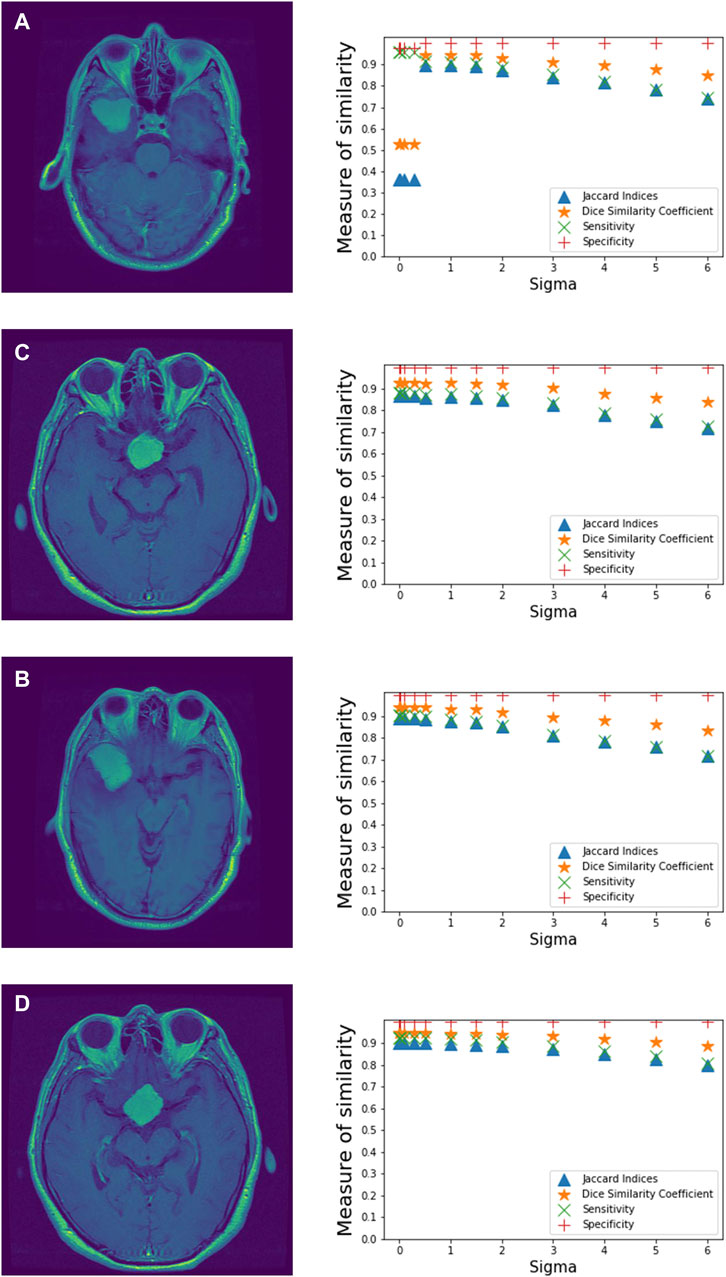
FIGURE 9. Influence of sigma on the performance of the minimum spanning tree-based method. (A–D) Images and the corresponding graphs showing measures of similarity (vertical axis) of the segmented images using the minimum spanning tree method in relation to the tuned sigma (horizontal axis). The sigma values tested include: 0, 0.01, 0.1, 0.3, 0.5, 1.0, 1.5, 2.0, 3.0, 4.0, 5.0, and 6.0.
3.4.1 Time Complexity Analysis
The time complexity for the graph construction is documented by Virtanen et al. (2020) and the time complexity construction of the MST is described (Pettie and Ramachandran, 2002). The implementation was done by writing scripts in the python programming language, and it was run on a PC processor (Core i7-8650UCPU @ 1.90GHz × 8). The input size is defined by the number of pixels in the image, corresponding to vertices in the graph. The largest size of the images segmented is 512 × 512, which gives less than 300,000 vertices. The proposed method can construct a graph and MST of more than 1,000,000 vertices in less than a second, illustrated in Figure 10.
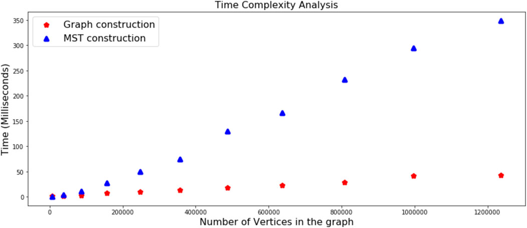
FIGURE 10. Time complexity analysis. The time spent on graph construction is less than the time spent on minimum spanning tree (MST) construction. The computation time increases based on the size of the input image.
4 Discussion
Brain tumor segmentation is a tedious task, especially when the tumor is in brain regions with highly complex tissue structures. Some of the obstacles listed in different literature include the skin, fat, muscle, neck, and eyeballs because they hinder automatic segmentation of the brain tumors. In addition, the quality of the images could compromise the results. Here, we propose an MST-based approach for segmenting the region of interest interactively.
In this paper, we have applied the MST-based approach to segment brain tumors in human patient MRI data set and compared the results to the ground truth. Figure 2 summarizes the steps used for segmenting the brain tumor interactively. Figure 3 demonstrates the strength of the MST approach by comparing our results to the ground truth provided in the data set. All the slices are transverse (axial) planes from different patients showing different tumor locations. Most of the tumors in these slices have clear boundaries and can be segmented by applying a small sigma value in the preprocessing step.
Additionally, we test the approach by segmenting the brain from the non-brain tissue. The brain is segmented by clicking inside the brain and then on the skull. The MST efficiently extracts the brain referred to in Figure 4. We compare the obtained results to the ground truth of the brain materials. We use the known labels of the brain tissues given in the data as the ground truth and the approach gives promising results.
Also, we assess the impact of filtering the image before segmenting the ROI. The results in Figure 5 indicate that the choice of sigma can highly influence the segmented tumor. Therefore, the parameter sigma needs to be tuned carefully, which is disadvantageous because the MST must be reconstructed every time sigma is changed. To reduce the burden of trial and error, we utilize the efficiency of the MST approach to segment the tumor without having to tune parameters repeatedly. Figure 6 shows the results of the segmented tumor obtained interactively without changing the values of sigma. Figure 6F shows how labels were changing. The advantage of the interactive part is that the MST is constructed only once and we keep updating the same MST. The MST approach requires a boundary between the ROI and the background. A single step is enough to segment the tumor for images whose regions of interest are well separated from the background. The method works for images with weak boundaries between the region of interest and the background, but one may need more interactive steps to segment the tumor. If the region of interest is strongly connected to the background, meaning that there is no boundary between them, the method will fail.
Further, we present results for the tumor being at a complicated location in Figure 7. We visualize the results in each step showing how the tumor was being detached from other brain materials and non-brain materials. We apply a sigma of 0.9 in the preprocessing step and then construct the MST. We run the interactive part and isolate the tumor by continuously splitting the MST. The approach segments the tumor efficiently.
In each of the segmented results, we provide a summary for the performance analysis of the MST. We use Jaccard indices, Dice similarity coefficients, sensitivity, and specificity to evaluate the performance of the MST-based approach. The results are summarized in Tables 1, 2. In Table 2 we compare the results obtained by using the MST-based method to the results obtained by Kasar et al. (2021) using the same data set. Also, Figures 8, 9 present results by testing different values of sigma that can give a good performance of the approach. The results indicate that for images whose ROI is well separated from the background, a sigma value close to zero can give good results. For images whose tumors are in complex locations, tuning parameters in the preprocessing step can be challenging.
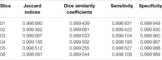
TABLE 1. The performance of the minimum spanning tree approach based on data set number two, presented using Jaccard Indices, Dice Similarity Coefficients, Sensitivity, and Specificity.

TABLE 2. The performance of the minimum spanning tree approach compared to UNET and SEGNET based on data set number one, presented using average in each measure of similarity.
In the analysis, we only used a Gaussian filter. However, other filters can be tested to check if they can give better results, depending on the quality of the image and the complexity of the tumor’s location. The implementation was done by writing scripts in the python programming language. Figure 10 gives the time complexity analysis for graph and MST construction. The link for the code used is available in the data availability section, as well as the links for the data used in this paper. As pointed out in the gland challenge of image processing, the availability of large public datasets is highly desirable Dufaux (2021) especially with their gold standard for testing different algorithms. Most freely available image data sets do not contain ground truth segmentation.
Data Availability Statement
The links for the datasets analyzed for this study can be found in (Cheng, 2017) (first data set) and (Aubert-Broche et al., 2006; Cocosco et al., 1997) (second data set). The code used for producing the result is freely available here https://github.com/simeonmayala/minimum-spanning-tree-segmentation.
Author Contributions
All authors conceptualized the study and made significant contributions to the manuscript. SM conducted the analysis to produce the results and put forward the proposed draft of the manuscript; IH, JH, and SA contributed in writing, editing, creation of figures, and provided knowledge support of the biological concepts. SG and MB supervised the work including writing, reviewing, and editing.
Funding
The project is funded by the University of Bergen, Bergen, Norway.
Conflict of Interest
The authors declare that the research was conducted in the absence of any commercial or financial relationships that could be construed as a potential conflict of interest.
Publisher’s Note
All claims expressed in this article are solely those of the authors and do not necessarily represent those of their affiliated organizations, or those of the publisher, the editors and the reviewers. Any product that may be evaluated in this article, or claim that may be made by its manufacturer, is not guaranteed or endorsed by the publisher.
Acknowledgments
The preprint version of (Kasar et al., 2021) was included for data comparison.
Supplementary Material
The Supplementary Material for this article can be found online at: https://www.frontiersin.org/articles/10.3389/frsip.2022.816186/full#supplementary-material
References
Aubert-Broche, B., Evans, A. C., and Collins, L. (2006). A New Improved Version of the Realistic Digital Brain Phantom. NeuroImage 32, 138–145. doi:10.1016/j.neuroimage.2006.03.052
Banerjee, S., Mitra, S., and Uma Shankar, B. (2016). Single Seed Delineation of Brain Tumor Using Multi-Thresholding. Inf. Sci. 330, 88–103. doi:10.1016/j.ins.2015.10.018
Cheng, J., Huang, W., Cao, S., Yang, R., Yang, W., and Yun, Z. (2015). Enhanced Performance of Brain Tumor Classification via Tumor Region Augmentation and Partition. PloS one 10, e0140381. doi:10.1371/journal.pone.0140381
Cheng, J., Yang, W., Huang, M., Huang, W., Jiang, J., Zhou, Y., et al. (2016). Retrieval of Brain Tumors by Adaptive Spatial Pooling and fisher Vector Representation. PloS one 11, e0157112. doi:10.1371/journal.pone.0157112
Cheriton, D., and Tarjan, R. E. (1976). Finding Minimum Spanning Trees. SIAM J. Comput. 5, 724–742. doi:10.1137/0205051
Ciesielski, K. C., and Udupa, J. K. (2011). A Framework for Comparing Different Image Segmentation Methods and its Use in Studying Equivalences between Level Set and Fuzzy Connectedness Frameworks. Computer Vis. Image Understanding 115, 721–734. doi:10.1016/j.cviu.2011.01.003
Cocosco, C. A., Kollokian, V., Kwan, R. K.-S., Pike, G. B., and Evans, A. C. (1997). “Brainweb: Online Interface to a 3d Mri Simulated Brain Database,” in NeuroImage (Citeseer).
Dale, A. M., Fischl, B., and Sereno, M. I. (1999). Cortical Surface-Based Analysis: I. Segmentation and Surface Reconstruction. Neuroimage 9, 179–194. doi:10.1006/nimg.1998.0395
Felzenszwalb, P. F., and Huttenlocher, D. P. (2004). Efficient Graph-Based Image Segmentation. Int. J. Comput. Vis. 59, 167–181. doi:10.1023/b:visi.0000022288.19776.77
Hahn, H. K., and Peitgen, H.-O. (2000). “The Skull Stripping Problem in Mri Solved by a Single 3d Watershed Transform,” in International Conference on Medical Image Computing and Computer-Assisted Intervention (Springer), 134–143. doi:10.1007/978-3-540-40899-4_14
Hua, R., Huo, Q., Gao, Y., Sui, H., Zhang, B., Sun, Y., et al. (2020). Segmenting Brain Tumor Using Cascaded V-Nets in Multimodal Mr Images. Front. Comput. Neurosci. 14, 9. doi:10.3389/fncom.2020.00009
Huang, H., Yang, G., Zhang, W., Xu, X., Yang, W., Jiang, W., et al. (2021). A Deep Multi-Task Learning Framework for Brain Tumor Segmentation. Front. Oncol. 11. doi:10.3389/fonc.2021.690244
Iglesias, J. E., Liu, C.-Y., Thompson, P. M., and Tu, Z. (2011). Robust Brain Extraction across Datasets and Comparison with Publicly Available Methods. IEEE Trans. Med. Imaging 30, 1617–1634. doi:10.1109/tmi.2011.2138152
Kalavathi, P., and Prasath, V. S. (2016). Methods on Skull Stripping of Mri Head Scan Images—A Review. J. digital Imaging 29, 365–379. doi:10.1007/s10278-015-9847-8
Kang, B. (2021). “Exploring Graph-Based Neural Networks for Automatic Brain Tumor Segmentation,” in From Data to Models and Back: 9th International Symposium, DataMod 2020, Virtual Event, October 20, 2020 (Springer Nature), 18. Revised Selected Papers.12611
Kasar, P. E., Jadhav, S. M., and Kansal, V. (2021). Mri Modality-Based Brain Tumor Segmentation Using Deep Neural Networks. doi:10.21203/rs.3.rs-496162/v1
Long, X., and Sun, J. (2020). Image Segmentation Based on the Minimum Spanning Tree with a Novel Weight. Optik 221, 165308. doi:10.1016/j.ijleo.2020.165308
Lundh, F. (1999). An Introduction to Tkinter. Available at:www.pythonware.com/library/tkinter/introduction/index.htm
Morris, O., Lee, M. d. J., and Constantinides, A. (1986). Graph Theory for Image Analysis: an Approach Based on the Shortest Spanning Tree. IEE Proc. F (Communications, Radar Signal Processing) (Iet) 133, 146–152. doi:10.1049/ip-f-1.1986.0025
Nandi, A. K. (2021). Apropos of Signal Processing. Front. Signal Process. doi:10.3389/frsip.2021.686341
Pettie, S., and Ramachandran, V. (2002). An Optimal Minimum Spanning Tree Algorithm. J. ACM (Jacm) 49, 16–34. doi:10.1145/505241.505243
Roy, S., and Maji, P. (2015). “A Simple Skull Stripping Algorithm for Brain Mri,” in 2015 Eighth International Conference on Advances in Pattern Recognition (ICAPR), 1–6. doi:10.1109/ICAPR.2015.7050671
Saglam, A., and Baykan, N. A. (2017). Sequential Image Segmentation Based on Minimum Spanning Tree Representation. Pattern Recognition Lett. 87, 155–162. doi:10.1016/j.patrec.2016.06.001
Ségonne, F., Dale, A. M., Busa, E., Glessner, M., Salat, D., Hahn, H. K., et al. (2004). A Hybrid Approach to the Skull Stripping Problem in Mri. Neuroimage 22, 1060–1075. doi:10.1016/j.neuroimage.2004.03.032
Smith, S. M. (2000). Bet: Brain Extraction Tool. FMRIB TR00SMS2b, Oxford Centre for Functional Magnetic Resonance Imaging of the Brain). Headington, UK: Department of Clinical Neurology, Oxford University, John Radcliffe Hospital.
Urquhart, R. (1982). Graph Theoretical Clustering Based on Limited Neighbourhood Sets. Pattern recognition 15, 173–187. doi:10.1016/0031-3203(82)90069-3
Virtanen, P., Gommers, R., Oliphant, T. E., Haberland, M., Reddy, T., Cournapeau, D., et al. (2020). SciPy 1.0: Fundamental Algorithms for Scientific Computing in Python. Nat. Methods 17, 261–272. doi:10.1038/s41592-019-0686-2
Wang, L., Wang, S., Chen, R., Qu, X., Chen, Y., Huang, S., et al. (2019). Nested Dilation Networks for Brain Tumor Segmentation Based on Magnetic Resonance Imaging. Front. Neurosci. 13, 285. doi:10.3389/fnins.2019.00285
Xu, Y., and Uberbacher, E. C. (1997). 2d Image Segmentation Using Minimum Spanning Trees. Image Vis. Comput. 15, 47–57. doi:10.1016/s0262-8856(96)01105-5
Keywords: brain tumor, brain tumor segmentation, minimum spanning tree, segmentation, image processing
Citation: Mayala S, Herdlevær I, Haugsøen JB, Anandan S, Gavasso S and Brun M (2022) Brain Tumor Segmentation Based on Minimum Spanning Tree. Front. Sig. Proc. 2:816186. doi: 10.3389/frsip.2022.816186
Received: 16 November 2021; Accepted: 31 January 2022;
Published: 11 March 2022.
Edited by:
Tao Lei, Shaanxi University of Science and Technology, ChinaReviewed by:
Zhenghao Shi, Xi’an University of Technology, ChinaBaha Şen, Yıldırım Beyazıt University, Turkey
Copyright © 2022 Mayala, Herdlevær, Haugsøen, Anandan, Gavasso and Brun. This is an open-access article distributed under the terms of the Creative Commons Attribution License (CC BY). The use, distribution or reproduction in other forums is permitted, provided the original author(s) and the copyright owner(s) are credited and that the original publication in this journal is cited, in accordance with accepted academic practice. No use, distribution or reproduction is permitted which does not comply with these terms.
*Correspondence: Simeon Mayala, c2ltZW9uLm1heWFsYUB1aWIubm8=