Speech Localization at Low Bitrates in Wireless Acoustics Sensor Networks

The use of speech source localization (SSL) and its applications offer great possibilities for the design of speaker local positioning systems with wireless acoustic sensor networks (WASNs). Recent works have shown that data-driven front-ends can outperform traditional algorithms for SSL when trained to work in specific domains, depending on factors like reverberation and noise levels. However, such localization models consider localization directly from raw sensor observations, without consideration for transmission losses in WASNs. In contrast, when sensors reside in separate real-life devices, we need to quantize, encode and transmit sensor data, decreasing the performance of localization, especially when the transmission bitrate is low. In this work, we investigate the effect of low bitrate transmission on a Direction of Arrival (DoA) estimator. We analyze a deep neural network (DNN) based framework performance as a function of the audio encoding bitrate for compressed signals by employing recent communication codecs including PyAWNeS, Opus, EVS, and Lyra. Experimental results show that training the DNN on input encoded with the PyAWNeS codec at 16.4 kB/s can improve the accuracy significantly, and up to 50% of accuracy degradation at a low bitrate for almost all codecs can be recovered. Our results further show that for the best accuracy of the trained model when one of the two channels can be encoded with a bitrate higher than 32 kB/s, it is optimal to have the raw data for the second channel. However, for a lower bitrate, it is preferable to similarly encode the two channels. More importantly, for practical applications, a more generalized model trained with a randomly selected codec for each channel, shows a large accuracy gain when at least one of the two channels is encoded with PyAWNeS.

1 Introduction

There are over 50 billion mobile devices connected to the cloud as of 2020 (Yang and Li, 2016), out of which more than 50% are estimated to be the Internet of Things (IoT) and wireless acoustic sensor network (WASN) devices (The Cisco Visual Networking Index, 2020). We can consequently expect that services based on WASN technology will be increasingly rolled out, not only for low latency and high communication bandwidth, but also to gain access to multiple sensors for cooperative localization strategies. In fact, such WASN ecosystems will enhance various context-aware and location-based applications for which real-time localization is becoming increasingly beneficial especially in the development of smart devices and voice interfaces. However, WASN-based systems have to use communication protocols to transmit data between nodes, where codecs inevitably introduce noise in the received signals and reduce the accuracy of subsequent localization modules. While both speech and audio codecs (e.g., (Bäckström, 2017)) and localization methods (e.g., Cobos et al. (2017)) are well-studied, their combined effect has not received much attention. Therefore, there is a need for localization methods specifically designed for encoded signals.

Many methods have been previously developed to solve target localization problems in WASNs by focusing on estimating the source’s coordinates. The established methods could be classified depending on the used measurement models: 1) Time Difference of Arrival (TDoA); 2) distance measurement; 3) received signal strength; 4) direction of arrival (DoA) also known as bearing, measurements; and 5) signal energy and their combinations. Each measurement has its own merits, and this paper focuses on DoA. The proposed method estimates the azimuth angle of a target source referring to a pair of sensors. Unfortunately, due to the limited energy and bandwidth of the fused signals, the traditional DoA-based localization methods usually fail to achieve satisfactory accuracy. Alternatively to conventional localization methods, much faster neural network (NN)-based methods have also shown their potential application in DOA estimation in recent literature, where specific extracted features are used as the input for a multilayer neural network to learn the nonlinear mapping from such features to the DoA estimation (Xiao et al., 2015; Pertilä and Parviainen, 2019). The high accuracy of learning based methods is due to the constrained training datasets, targeting specific use cases. Such systems’ performance significantly drops when used in conditions that do not match the training domain. This mismatch problem has been widely studied in the context of robustness to background noise and/or reverberation (Xiao et al., 2015; Chakrabarty and Habets, 2017; Huang et al., 2018; Liu, 2020), array imperfections (Liu et al., 2018), multiple sources scenario (Takeda and Komatani, 2016; Chen et al., 2018). However, as far as we know, prior works have not addressed distortions due to codecs.

The proposed localization scheme is motivated by the speech codec we recently published (Bäckström et al., 2021), where we estimated the TDoA from a multi-channel, coded mixture. This method of front-end processing opens up avenues for processing audio not just from microphones from the same sensor array but from microphones from distinct devices. In parallel, the popularity of voice-enabled devices opens up an interesting area of research. However, we also need to take into account that different devices from different manufacturers may not support the same encoding standards. To leverage a specific two-channel scenario, there are two options, both with their particular trade-offs: 1) One of the recording devices can also be a fusion center (FC), responsible for receiving and decoding the second signal then processing with localization, as in Figure 1A. 2) Alternatively, the two devices can both just record the signal and send the encoded version to the FC for localization, as in Figure 1B. In both scenarios, the device can compress the signals before transmission to minimize the amount of transmitted data. However, distributed sensing with quantization and coding is a complex multi-objective optimization problem (Shehadeh et al., 2018). The computational load, power consumption, bandwidth, signal accuracy, and localization accuracy should all be simultaneously optimized while we also have to take into account the individual limits of each device. With this motivation, in contrast to prior studies and, in addition to environmental and sensor noise, in this work, we focus on the effect of quantization noise on localization accuracy. To build our localization model, we pool training data from several sources, and simulate varying bitrate and codecs conditions (Figure 2). Since noise robustness has received a lot of attention in the literature, we focus primarily on the less explored area of robustness with respect to codecs.

FIGURE 1

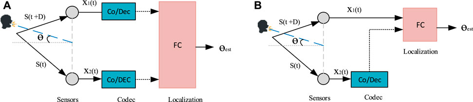
FIGURE 1. Generic system models: (A) Two encoded-channel model: The two devices just records the signal and sends the encoded signal to the FC. (B): Single encoded-channel model: One of the recording device itself is the FC.

FIGURE 2

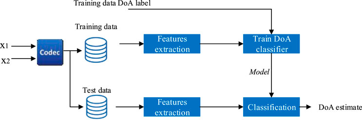
FIGURE 2. System diagram of the proposed learning-based approach for DoA estimation.

Prior work in this area has focused on examining the effect of mixed bandwidths on automatic speech recognition (Mac et al., 2019) as well as evaluating the performance of different audio codecs on emotion recognition (Garcia et al., 2015; Siegert et al., 2016). Evaluation of the audio quality of codecs is naturally also a classic task, e.g. Rämö and Toukomaa (2015).

In this paper, we consider a speaker target positioning as a DoA classification task. Our contribution is to study how our recently proposed simple DNN architecture (Zarazaga et al., 2020) performance varies with the different bitrate encoding of recent communication codecs including PyAWNeS (Bäckström et al., 2021), OPUS (Valin et al., 2012), the Enhanced Voice Services (EVS) (Bruhn et al., 2012), and Lyra (Kleijn et al., 2021). We analyze the performance of both considered scenarios as a function of the audio input bitrate. We demonstrate that by training with low bitrates we can recover some of the localization performance loss. Motivated by the two-device context for DoA estimation, we also study the performance of our estimator if the two considered input channels to the network are not encoded with the same bitrate. Surprisingly, even though the model is trained with data encoded at a low bitrate, it works almost as well as the model trained with uncompressed data. Most interestingly, we get large accuracy gains for a randomly chosen codec at low bitrates by using the PyAWNeS codec for low bitrate training, suggesting that it preserves spatial information even in low bitrate conditions.

2 Problem Statement of Low Bitrate DOA Estimation

2.1 Data Model

Our particular focus in this paper is a typical home scenario, where a user has multiple, potentially wearable, audio devices near him. We consider the localization task in a two-dimensional area with a number of low-cost and randomly distributed sensors. The sensors transmit their signals to the fusion center, which estimates the targets’ locations. This network configuration is required since typical DoA estimators require at least two channels. Specifically, we consider a wireless acoustic sensor network (WASN) of two local, independent sensors working together with a fusion center (FC).

The received signal in the m^th device can be modeled in the discrete-time Fourier transform (DTFT) domain as

$X_m\left(w\right)={\beta }_{m}S\left(w\right)\exp \left(-jw{\tau }_m\right)+ϵ\left(w\right),m=\left\{\mathrm{1,2}\right\},(1)$

where S(ω) is the spectrum of the target speaker, attenuated with a positive amplitude decay factor β_m ∈ I R+, and delayed by a transmission time of flight (ToF) τ_m ∈ I R+ relative to the speaker position. Moreover, ϵ(w) stands for noise and reverberation measurements and $j=\sqrt{(-1)}$ is the imaginary unit. The time delay of arrival (TDoA) parameter (τ₁ − τ₂), referring to the two channels X₁ and X₂, represents the source’s spatial location information.

In real-life WASNs applications, the individual sensor signals have to be quantized and coded with a finite bitrate. The decoded outputs of each sensor can, accordingly, be assumed to be non-linear transformations of the original, which likely degrade the signal quality. Consequently, quantization can distort and bias the information needed for localization, especially at low bitrates.

3 System Description

3.1 Overview

Our localization estimator is similar to the system described in Zarazaga et al. (2021), previously used to model the distribution of various spatial cues using a two-channel DNN-based architecture as shown in Figure 3. The model parameters are estimated by using the probability at each time-frequency point that a target speaker comes from a given DoA. First, the STFT is performed on the left and right channels to obtain the time-frequency representation of the input signals, here denoted as X₁, and X₂ respectively, where t = 1, …, T is the frame index and b = 1, …, B is the frequency bin index. The resulting spectrum is a (T × B) complex-valued matrix, where T represents the number of time frames contained in the audio sequence and B is the number of frequency bins.

FIGURE 3

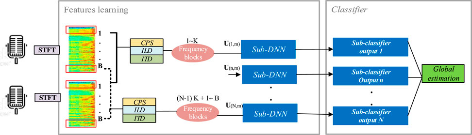
FIGURE 3. Proposed workflow.

FIGURE 4

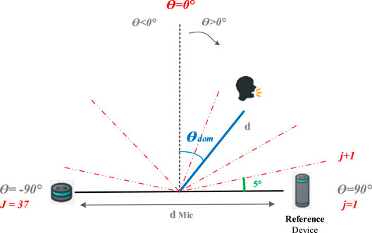
FIGURE 4. The space is divided into J parts. The elements of the ground-truth range in [1..J] Adapted from Zarazaga et al. (2021).

3.2 Input Feature Set

The input feature set has critical significance for a DNN-based estimator. Clearly, the feature set should include the required DoA information. However, with quantized signals, we expect that information in some frequency bands could be lost at low bitrates, which can distort feature extraction and bias the model. Therefore, we have decided to slide our input features into uniformly distributed frequency blocks from which we can detect the DoA information in each frequency band. The input features are estimated at each time-frequency unit and grouped into N uniformly distributed frequency blocks, each of them containing $K=\lceil \frac{B}{N}\rceil$ frequency bins. In our two-device model, we have chosen to use the inter-channel level difference (ILD), inter-channel phase difference (IPD), and the phase transform (PHAT) cross-power spectrum (CPS) across all frequency bins in the STFT domain as inputs to the neural network in a given time frame. This choice is motivated by the fact that the combination of CPS, ITD and ILD can make the estimation of sound source direction more accurate. Thus, we use a feature vector combining ITD, ILD and CPS derived from the observed input spectrum in each frequency block, consecutively defined as

$ILD\left(t,b\right)=20{\log }_{10}\left(\frac{|X_2\left(t,b\right)|}{|X_1\left(t,b\right)|}\right),\in {\mathbb{R}}^{TXB},(2)$

$CPS\left(t,b\right)=\frac{X_1\left(t,b\right)X_2^{*}\left(t,b\right)}{|X_1\left(t,b\right)X_2^{*}\left(t,b\right)|},\in {\mathbb{R}}^{TXB},(3)$

and

$ITD\left(t,b\right)=\underset{t}{\mathrm{argmax}}\left(CPS\left(t,b\right)\right),\in {\mathbb{R}}^{TXB},(4)$

where |.| takes the absolute value of their arguments, and argmax computes the time lag of the maximum peak. Concatenating CPS, ILD and ITD features, a vector is obtained at each time-frequency unit $U(t,b)={[CP{S}^T(t,b),IL{D}^T(t,b),IT{D}^T(t,b)]}^T\in {\mathbb{R}}^{Tx3B}$. All extracted vectors of features are split into N uniformly distributed frequency blocks (only along the frequency bins), each of them containing $K=\lceil \frac{B}{N}\rceil$ frequency bins, where each block involves only the information from K frequency bins as follows:

$U_{\left(t,n\right)}={\left[U^T\left(t,\left(n-1\right)K+1\right),\dots ,U^T\left(t,nK\right)\right]}^T\in {\mathbb{R}}^{3K},(5)$

where n is the index of the n^th frequency block fed into the n^th DNN. The STFT of the raw data at a sampling frequency of 16 kHz is computed in frames of 2048 samples (128 ms) with a 50% overlap. A sliding frequency window with 64 samples and a 50% overlap is then used to extract 31 CPS vectors in each time frame, which are then cropped to a number of samples equivalent to a maximum microphone distance of around 2.5  m. Therefore, the CPS vector within a lag range of [ − 128, + 128] samples has a size of 256. Then, adding then ILD for 64 time-frequency units and one ITD value results in an input feature vector U_(t,n) with length Q = 321 for each DNN.

3.3 Target Outputs

We define the DoA estimation as a classification task on a predefined grid of angles, corresponding to the likelihood of an active source at each angle. For that, we use a uniform azimuth grid which stands for the azimuth directions θ_j from −90° to +90° with the desired grid resolution of 5° (Figure 4). Thus, the resulting grid contains $n_{DoA}={\sum }_{j=0}^{J}j$ points. The target of each DNN is a binary vector of size n_DoA × 1 , where each index corresponds to one discrete DoA. Only the element of the output DoA vector that is the closest to the ground-truth DoA value is set to 1.

3.4 Model Architecture

The neural network architecture is illustrated in Figure 5. It consists of one input layer representing the low-level extracted features followed by two hidden layers of sparse autoencoders (AEs) (Bengio et al., 2013), and the fourth layer uses a softmax classifier to estimate a set of probabilities that the current input is oriented toward potential DoAs. The first input layer represent the extracted low-level features. Therefore, the number of input neurons equals the dimension of the feature vector, Q = 321 neurons, and one bias unit. The second part uses this low level feature input layer to extract high-level features. Following (Yu and Deng, 2011), we use two hidden sparse AEs which are composed of V = 256 neurons and one bias unit employing a sigmoid activation function. The estimated high level-features will serve as input for the fourth layer to estimate the DoAs, using a softmax layer containing 37 neurons corresponding to the n_DoA considered angles. Thus, our DNN outputs 37 nodes, which represent the azimuth directions θ_j from −90° to +90° with steps of 5°, representing the likelihood of the presence of a sound source P = {p_j} in the j^th orientation index. The target of the DNN is a binary vector of size n_DoA × 1, where each index corresponds to one discrete DoA. For each active source, the element of the target vector that is the closest to the true DoA is set to 1. When several sources are present in the scene, more than one neuron can be activated (set to 1). All other target outputs are inactive (set to 0).

FIGURE 5

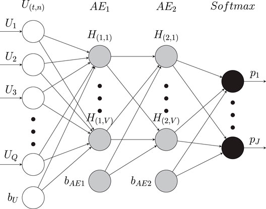
FIGURE 5. Architecture of the used DNN_n: U_n,m is the input vector of features and a bias vector b_U. AE₁ and AE₂ are two auto encoders and the bias vectors $b_{A{E}_1}$ and $b_{A{E}_2}$. The softmax classifier gives the probability p_j = j|U_t,m.

3.5 From Sub-classifier to Global DoA Classifier

In the proposed strategy, each well-trained DNN is fed with the input features from each time-frequency unit, and then the posterior probability of the sound source in each angle is obtained. After that, the average posterior probability of each direction in all frames is calculated, and the azimuth corresponding to the maximum posterior probability is taken as the localization result.

4 Experimental Settings for DOA Estimation

For our DoA estimation system evaluation, we first present the generated dataset made with the simulated spatial room impulse responses (SRIRs) that we used for training and testing. Then, we describe the DNN training procedure and settings for the following experiments.

4.1 Datasets

To train the networks, as well as for some test datasets, we synthesized SRIRs using Pyroomacoustics (Scheibler et al., 2017). The room size is 8×6×3  m³ with a reverberation time of about RT₆₀ = 0.3 s, with inter-sensor distance d_mic = [1, 2] m, and source-to-microphone distances d = [1, 2, 3] m. We synthesized all possible SRIRs for the room, corresponding to all DoAs. Anechoic utterances from the LibriSpeech dataset (Panayotov et al., 2015) were randomly extracted for both training and test sets. For the training dataset, for each configuration, we generate several stereo mixtures sampled at 16 kHz corresponding to all possible DoAs from −90° to +90° with steps of 5°. Each SRIR was convolved with a different 15 s speech signal randomly extracted from a subset of the LibriSpeech dataset.

4.2 Training Procedure

Similar to Yu and Deng (2011) and Dean et al. (2012), the process of training of each DNN is divided into pre-training and fine-tuning stages. In the pre-training phase, the AEs and softmax classifier are trained individually by using each output layer as an input for the next layer, fixing the weights of the previous layers at each stage. The greedy layer-wise training of Bengio et al. (2007) and Liu and Nocedal (1989) and the limited memory BFGS (L-BFGS) optimization algorithm are used to minimize the cost function. The unsupervised training of the two AEs outputs high-level features used to train the softmax classifier, which activates the j^th neuron, giving the highest probability that the current set U_(t,n) is oriented to the j^th direction. A cross-entropy loss function is therefore used to optimize the softmax classifier. The fine-tuning stage is the stacking and the training of the overall DNN. Hence, the AEs and the softmax classifier are stacked together. Then the overall DNN is trained employing L-BFGS optimization to minimize the difference between the DNN’s output and the label of the training dataset. The learning parameters for different training stages of the DNN are shown in Table 1.

TABLE 1

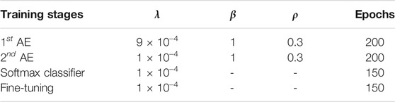
TABLE 1. List of training parameters for the different training stages of the DNNs, where λ is the weight decay, β is the sparsity penalty term and ρ is the sparsity parameter.

4.3 Codecs

To simulate a variety of audio codecs before transmission to the FC for localization, we encode and decode each waveform with a selected codec. Since we are interested in speech data, our investigations are focused on selected speech audio codecs. Namely, we use the 3GPP Enhanced Voice Services (EVS) codec (Bruhn et al., 2012), Opus (Valin et al., 2012), our own PyAWNeS-codec (Bäckström et al., 2021), and the neural codec Lyra (Kleijn et al., 2021). In particular,

•EVS has two operational modes: 1) the primary mode with 11 fixed bit rates ranging from 7.2 kB/s to 128 kB/s and one Variable BitRate (VBR) 5.9 kB/s. 2) the EVS AMR-WB Inter-Operable mode with 9 bitrates ranging from 6.6 kB/s to 23.85 kB/s. EVS supports four input and output sampling rates [8, 16, 32, 48] kHz. A delay compensation mode is integrated into the EVS codec, allowing the compensation of the integrated delay of about 32 ms within the encoded output signal.

•Opus is an open source codec developed by the Xiph.Org Foundation (Valin et al., 2012). It is based on a hybrid approach combining the speech-oriented SILK and the low-latency CELT. SILK is based on Linear Predictive Coding (LPC) and it is used for encoding information below 8 kHz. However CELT uses the modified discrete cosine transform (MDCT) in combination with the Code-excited Linear Prediction (CELP) frequency domain, and it is used to encode information above 8 kHz. The Opus supports bitrate ranging from 6 kB/s to 256 kB/s. Several versions of VBR and CBR operation are also available. The Opus codec supports the sampling rates 8, 12, 16, 24 and 48 kHz, with automatic resampling where needed. The Opus codec internally decided at which bandwidth the codec operated at the target bitrate.

•The Python acoustic wireless network of sensors (PyAWNeS) codec is a speech and audio codec especially designed for distributed scenarios, where multiple independent devices sense and transmit the signal simultaneously (Bäckström et al., 2021). In contrast to prior codecs, it is designed to provide competitive quality in a single channel mode, but such that quality is improved with every added sensor. The codec is based on the TCX mode of the EVS codec (Bruhn et al., 2012), but uses dithered quantization to ensure that quantization errors in independent channels have unique information. Another novelty of the codec is that, although it has a reasonably conventional structure, it is implemented on a machine learning platform such that all parameters can be encoded end-to-end.

•Lyra is a generative low-bitrate speech codec, a neural audio codec adopting WaveGRU architecture targeting speech at 3 kB/s.

To evaluate quality, ten native bitrate modes were selected [8, 13.2, 16.4, 24.4, 32, 48, 64, 92, 128, 160] kB/s at a sampling frequency of 16 kHz. An informal analysis of variable and constant bitrate modes did not show any significant difference in DoA quality.

5 Experimental Evaluation

To determine the impact of coding on a DoA estimate, we evaluate the effect of quantization at a selection of bitrates and codecs on the performances of the proposed DNN framework.

5.1 Evaluation Metrics

To characterize DoA accuracy, we determine the mean absolute error (MAE), the root-mean-square error (RMSE), and the measurement success rate (MSR). The MAE and the RMSE between an estimated DOA $(\widehat{{\theta }_k})$ of the k^th ground-truth DoA value (θ_k) for the r^th test utterance are computed respectively as

$MA{E}_{\theta }=\frac{1}{RK}\sum _{r=1}^R\sum _{k=1}^K|{\theta }_k-{\widehat{{\theta }_k}}^{\left(r\right)}|,(6)$

and

$RMS{E}_{\theta }=\sqrt{\frac{1}{R}\sum _{r=1}^R\left(\frac{1}{K}\sum _{k=1}^K|{\theta }_k-{\widehat{{\theta }_k}}^{\left(r\right)}{|}^2\right)},(7)$

where R is the number of utterances in the test set, and K denotes the number of simulated DoAs for each utterance (K = 37).

The accuracy of our DoA estimator is measured as a percentage (%) by the MSR indicating a correctly estimated DoA within a certain angular error tolerance.

$MS{R}_{{\theta }_i}=100\frac{m_k}{R},(8)$

where m_k denotes the number of successful tests of the k^th DoA angle. Due to the chosen DNN-based classifier’s output grid resolution, we consider a tolerance of up to 5°. This implies that DoA accuracy also reports the classification accuracy. Thus m_k is effective if and only if $|{\theta }_k-{\widehat{{\theta }_k}}^{(r)}|<$5°.

5.2 Model Performance as a Function of the Encoding Bitrate

We first investigate the performance of DNN in the simplest situation where two signals are similarly encoded with the same bitrate. For this experiment, we train our model without a codec using as input audio mixtures generated from a synthesized SRIR dataset, as explained in Section 4.1, resulting in a total of 74 SRIRs. Each SRIR was convolved with a different 1 s speech signal randomly extracted from a subset of the LibriSpeech dataset including 28, 539 audio files. Eight audio stereo recordings 15  s in duration were generated for each SRIR, resulting in 5 h of uncompressed data speech for the training set. For our test set, we generate both uncompressed data audio, and their encoded version. Hence, we generate four test set resulting from using PyAWNeS, OPUS, EVS, and Lyra codecs, including uncompressed and encoded versions of the audio. Ten bitrates [8, 13.2, 16.4, 24.4, 32, 48, 64, 92, 128, 160] kB/s are considered for the codecs used, except for EVS, which is limited to 128 kB/s, and Lyra, which only operates at 3 kB/s. The generated data resulted in 54 h of speech for each test set.

We first evaluated the DoA estimation performance of the trained DNN to return the DoA of uncompressed (high bitrate) data. Figure 6E represent the DoA accuracy through a probability matrix by matching the ground-truth potential DOAs to their predicted values. It represents the probability for the target DoA. It is computed by averaging the frequency dimension and the number of consecutive frames within the same test set J. As expected, the position of the target speaker varies from −90° to +90°. The different colours show the occupation probabilities for the target. We observe that the proposed DoA classifier shows a high similarity between the ground-truth DoA and the predicted labels. Accuracy is highest at relatively small azimuth angles (−45° < DoAs < 45°); however, slightly smaller accuracy is shown for higher azimuth orientation. Nevertheless, the DoA mismatch corresponds approximately to the 1 range. This is due to the mapping function between the input features vector and output angles, which is expected as an arcsin whose gradient $f^{\prime }(\sin \widehat{\theta })=\frac{1}{\cos \widehat{\theta }}$ approaches infinite when θ is large, resulting in a very sharp function that is quite hard for the DNN to fit. So the mapping function f will deviate from arcsin at a large azimuth and result in considerable bias estimations over 75°.

FIGURE 6

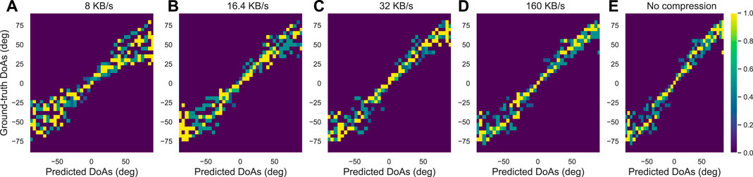
FIGURE 6. The localization accuracy of the DNNs: Similarity between Ground-truth DoAs (deg) and Predicted DoAs (deg) ranging from −90° to +90° when tested over: (A–D) PyAWNeS test set at various bitrates [8, 16.4, 32, 160] kB/s and (E) over test set without compression (No compression).

To study the effect of bitrate on DoA estimation, we use the encoded data from the PyAWNeS test set to plot the probability matrix for bitrates [8, 16.4, 32, 160] kB/s, figuring respectively in Figures 6A–D. Considering the generic system of Figure 1A, the test set is constructed where similar bitrates are chosen for both channels. We can notice a remarkable deviation of the estimated DoAs from the bisector proving a considerable degradation when the number of available bits for encoding the data is decreasing, especially at high DoAs.

To visualize the impact of the codec’s type and the used bitrate on DoA estimation performance, we analyze the absolute angular error over all potential DoAs and we take the model performance over test data without compression as our baseline accuracy. Figure 7 illustrates the performance of the DoA estimator with a boxplot of absolute angular error, as a function of the bitrate when the input channels are encoded using PyAWNeS, EVS, Opus, and Lyra. We observe that the DoA estimator is relatively robust at high bitrates and its accuracy degrades drastically only when going below 16.4 kB/s, where the angular error increases in comparison to the baseline estimator with uncompressed data. This is expected as the performance with low bitrate encoding introduces distortion in the speech characteristics and inevitably removes useful speech information. However, at higher bitrates, the degradation reduces to 40% relatively, and the distribution of angular error appears to be mostly independent of the bitrate when this latter exceeds 48 kB/s demonstrating that most of the speech characteristics required for spatial localization are preserved in this case. The histogram of the baseline and those of PyAWNeS, EVS and Opus, show approximately the same error distribution as the model trained and tested in high bitrate, matched conditions. The quartile and median values only slightly decrease for bitrates above 48 kB/s and stay concentrated within 1° of angular error. This demonstrates that the estimator is robust and consistent above 16.4 kB/s.

FIGURE 7

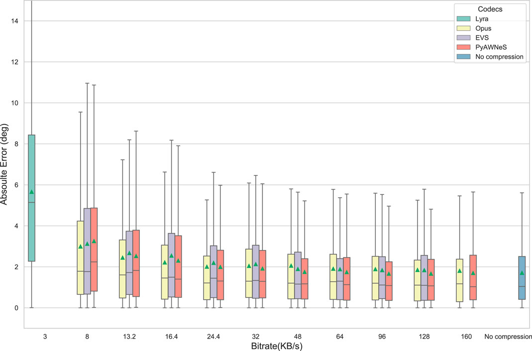
FIGURE 7. Absolute Error versus increasing bitrate when employing different codecs performed by the model trained without compression (w/o codec) on a test set including similarly encoded signals. The green triangle in each boxplot shows the MAE (deg).

To better visualize the effect of the used codec’s type on the DoA estimator, Figure 8 illustrates the degradation in relative root mean square error (RMSE) with the different bitrate audio inputs for our trained model by taking the angular error performed with uncompressed data as our baseline. As our results show, the relative RMSE increases sharply when the bitrate decreases. We can notice that the relative RMSE for the PyAWNeS codec is the best across all bitrates. However, both EVS and Opus result in higher relative RMSE. For 3 kB/s, Lyra results in high degradation, showing a relative RMSE exceeding 40°.

FIGURE 8

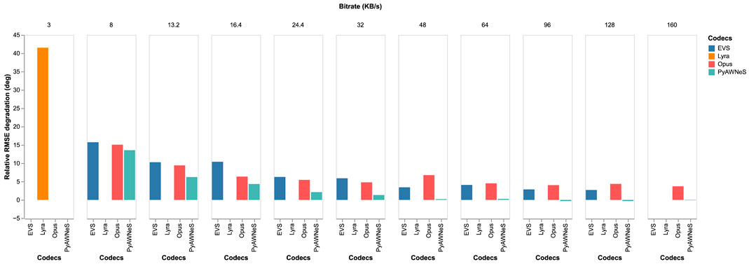
FIGURE 8. Relative RMSE (deg) versus an increasing bitrate (KB/s) performed by the model trained without compression (w/o codec) on a test set including similarly encoded signals.

To better understand this achievement, we also visualize the spectrum of an audio uncompressed example with various bitrates per channel, its corresponding frequency-slided CPS input feature, and the resulting TDoA between the two encoded channels for PyAWNeS codec in Figure 9. As can be seen, the frequency-slided CPS still involves the TDoA information between the two encoded channels over approximately all sub-bands [0, 31] for a bitrate up to 32 kB/s, which will make the performance of our DNN as efficient as for the uncompressed data. However, the CPS input feature loses its TDoA information for a lower bitrate. Hence, the localization information loss, especially at higher frequencies, is clear in both 16.4 kB/s and 8 kB/s encoding. Only lower frequencies over the first 7 sub-bands show the high peaks centered around the localization information. Similarly to the PyAWNeS spectrogram, we show this degradation in Figure 10 with the similar input and the same segment when using Opus. For a 32 kB/s, we notice many sidelobs in the frequency-slided CPS, resulting in a localization information loss over sub-bands. Moreover, as can be seen, that depending on the requested bitrate, the bandwidth can vary from narrowband (NB) to fullband (FB). In fact for the lowest bitrate of 8 kB/s, Opus encoding has no information above 4 kHz (NB), resulting in the highest peak centered around 0 (sample). There are also some aliasing artifacts apparent in the low frequencies, which causes the localization information inaccuracy. Similar to Opus, Figure 11 shows that even for high bitrates starting from 128 kB/s, introduced distortion in the EVS-coded spectrum results int high sidelobs in the input frequency-slided CPS feature even if we enabled EVS-SWB to encode up to 16 kHz. For 3 kHz, Lyra shows Figure 12 introduced distortion in the coded spectrum resulting in high sidelobs in the input frequency-slided CPS feature, which causes a localization information loss over almost all sub-bands.

FIGURE 9

FIGURE 9. 1^st row: Spectrograms for one uncompressed test utterance channel and its PyAWNeS-encoded versions at various bitrates [8, 16.4, 32, 160] kB/s. 2^nd row: Frequency-slided CPS input feature computed between two segments of the encoded channels. 3^rd row: argument of the maximum of CPS in each frequency band corresponding to the delay (samples) between the two channels.

FIGURE 10

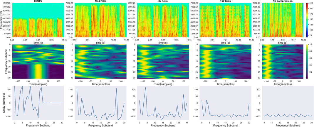
FIGURE 10. 1^st row: Spectrograms for one uncompressed test utterance channel and its Opus-encoded versions at various bitrates [160, 32, 16.4, 8] kB/s. 2^nd row: Frequency-slided CPS input feature computed between two segments of the encoded channels. 3^rd row: argument of the maximum of CPS in each frequency band corresponding to the delay (samples) between the two channels.

FIGURE 11

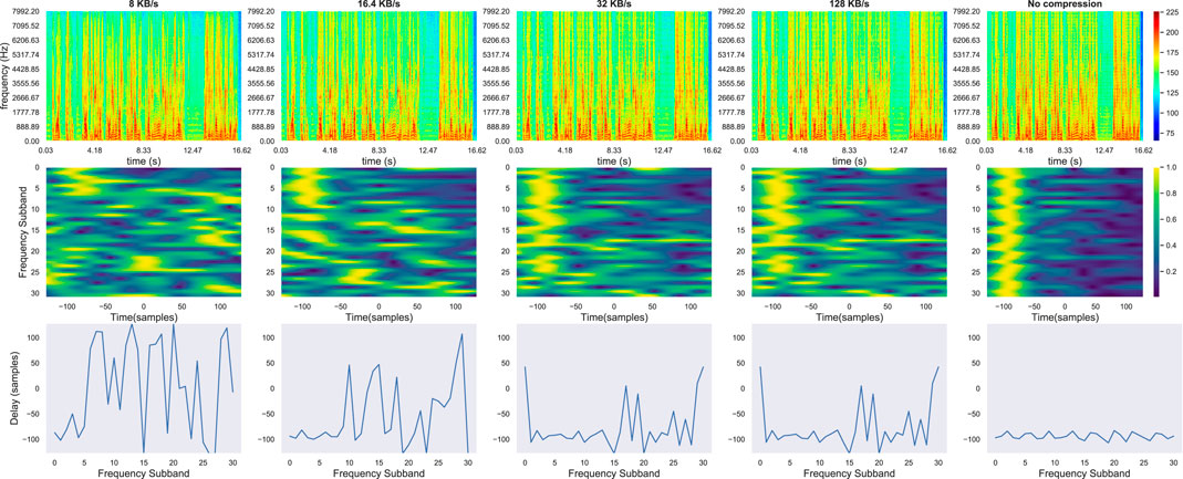
FIGURE 11. 1^st row: Spectrograms for one uncompressed test utterance channel and its EVS-encoded versions at various bitrates [8, 16.4, 32, 128] kB/s. 2^nd row: Frequency-slided CPS input feature computed between two segments of the encoded channels. 3^rd row: argument of the maximum of CPS in each frequency band corresponding to the delay (samples) between the two channels.

FIGURE 12

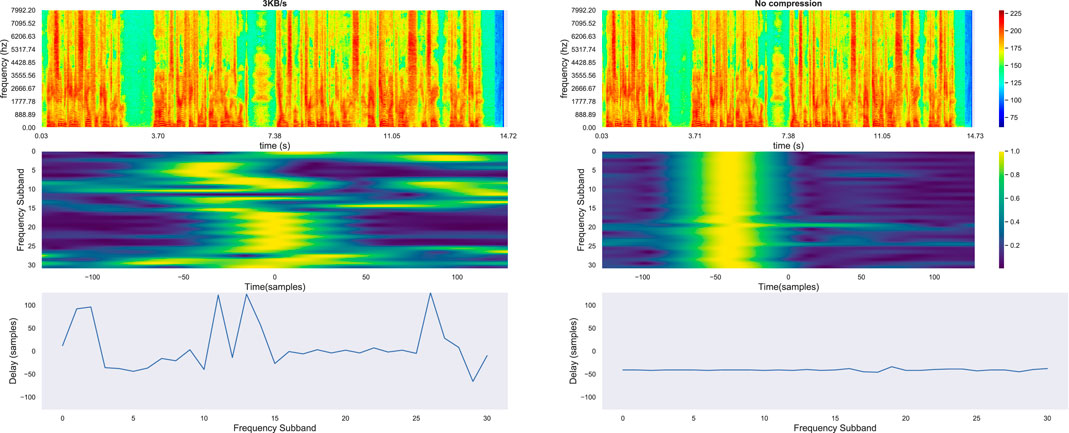
FIGURE 12. 1^st row: Spectrograms for one uncompressed test utterance channel and its Lyra-encoded versions at very low bitrate 3 kB/s. 2^nd row: Frequency-slided CPS input feature computed between two segments of the encoded channels. 3^rd row: argument of the maximum of CPS in each frequency band corresponding to the delay (samples) between the two channels.

5.3 Performance With Low Bitrate Training

In our second experiment, we wanted to explore if the degradation can be compensated by matching the training data with the test data. For this purpose, we did two different sets of experiments: First, we train individual two encoded channel models for low bitrate encoding at 8 and 16.4 kB/s. Then we analyzed to see if we can compensate for the degradation. Based on the first experiment, we employ the PyAWNeS codec to generate the train set as it outperforms Opus and EVS at a low bitrate.

Second, we trained a model with mixed bitrates. For each training example, we picked an encoding bitrate from the set [16.4, 32, 128] kB/s. For a fair comparison, the same number of training examples is used for training the mixed bitrate model and the low bitrate model.

Table 2 shows the results when the model is trained with a low bitrate PyAWNeS codec. For a better comparision we also report our results from Section 5.2, evaluating the model trained without a codec on different test sets under various codecs’ conditions: PyAWNeS, Opus, and EVS at [8, 16.4] kB/s, and Lyra at 3 kB/s. For the baseline model trained without codec, performance worsens as the bitrate decreases since lower bitrates imply more lossy encoding. As expected, the training with a matched bitrate makes the performance under seen (PyAWNeS) and unseen codecs (EVS and Opus) close to not using any codec, even at low bitrates. For EVS 8 kB/s, training with the codec at 16.4 kB/s improves MSR by almost 35%. However, this improvement is only up to 9.5% when training with a codec at 8 kB/s. In fact, it is shown that the degradation with the 8 kB/s is attributed to the loss of delay information in encoding that cannot be recovered by matching the test data with the 8 kB/s-trained model, which cannot see critical information for high frequencies during training and hence cannot recover the errors. Moreover, performance is much worse with the unmatched bitrate condition using the Lyra codec for which degradation could not be recovered. It is interesting to note, however, that the model trained with the 16.4 kB/s codec can perform better than the baseline matched trained model with the smallest RMSE 1.57° and highest accuracy of 99%.

TABLE 2

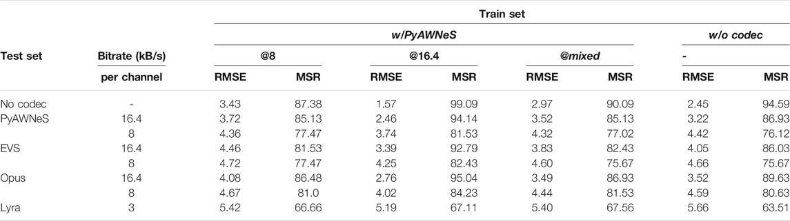
TABLE 2. Performance in terms of RMSE (◦) and MSR% in seen and unseen codecs conditions using the model serving as baseline trained without codec (w/o codec) and models trained with PyAWNeS at 16.4, 8 kB/s and mixed bitrate repectively named as (w/PyAWNeS@16.4), (w/PyAWNeS@8), (w/PyAWNeS@mixed).

The mixed bitrate model can not recover the degradation for all the different bitrate encodings we studied. For 16.4 kB/s, it is not as good as the matched training and is lower than the baseline.

5.4 Distributing Varying Bitrate Among the Two Channels

Previous experiments mainly focused on the condition of an equal bitrate for the two channels, so for the third part of this study, we wanted to find out if our two encoded-channel model trained without a codec can work well on the condition of a different bitrate based on the fact that the generic system model in Figure 1B is a specific case of Figure 1A, where the uncompressed channel could be simulated as a high bitrate encoded channel.

For this experiment, to simulate a test set for Figure 1B, we fix the input to one of the channels to be the uncompressed audio and vary the bitrate of the second channel.

In Table 3, we display RMSE and MSR performed by the baseline model without a codec (w/o codec) and the model trained with PyAWNeS at 16.4 kB/s (w/PyAWNeS@16.4) for different used codecs at different bitrates. It is interesting to note that for the model trained with 16.4 kB/s, the performance is better than the baseline matched trained model and can recover up to 100% of degradation in the case of the PyAWNeS and Opus 16.4 kB/s test sets.

TABLE 3

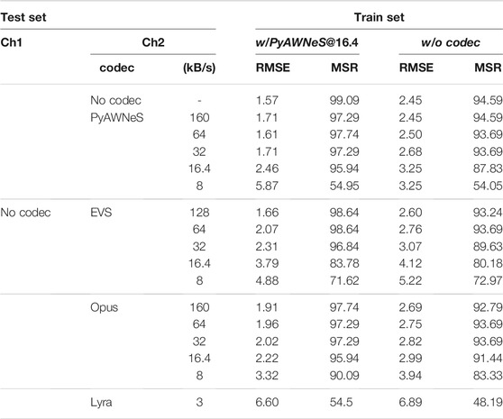
TABLE 3. Performance in terms of RMSE (◦) and MSR% in seen and unseen codecs conditions using the model serving as baseline trained without compression (w/o codec) and models trained with PyAWNeS at 16.4 (w/PyAWNeS@16.4).

We mention that even an internal delay introduced by codecs is already compensated for, and the EVS-encoded signals are still shifted by 21(samples), experimentally measured using a cross-correlation-based method. As we are considering both an uncompressed and coded mixture for this experiment, we manage to compensate for this delay in the test set so that the input ITD feature could be correctly computed for the model. This internal delay is independent of the bitrate and that is why its effect is not considered when both channels are encoded. On the other hand, some scale is noticed when decreasing the bitrate for all codecs. This will not affect the estimation when we similarly encode both channels, but it modifies the ILD input feature then biases the DoA estimation when these latter are encoded differently. In the experiment, we find that as expected, location information on the low bitrate 8 kB/s is often missed, which causes a large decrease.

To compare the two generic systems, we display the relative RMSE degradation performed by w/PyAWNeS@16.4 in Figures 13–16 presenting, respectively, the impact of PyAWNeS, Opus, EVS, and Lyra codecs at different bitrates when applied to one of the two channels and when the two channels are encoded. The angular error performed by the model with uncompressed audio for both channels is taken as our baseline. These results show that having one channel encoded with the highest bit rate is beneficial over encoding the two channels similarly. This demonstrates that the trained model performs better when there is at least one channel with no degradation rather than both channels having some degradation, even when the bitrate is as low as 32 kB/s. In fact, performance is better when the bitrate of one channel is greater than 32 kB/s as long as we retain a high bitrate on the other channel. However, when the bitrate for one channel gets as low as 16.4 kB/s, its is preferable to have two encoded channels, especially for both EVS and PyAWNeS. A similar achievement is also noticed at 3 kB/s when using Lyra.

FIGURE 13

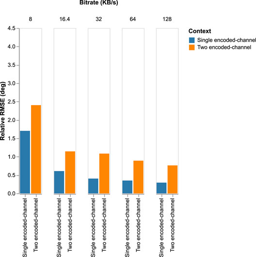
FIGURE 13. Relative RMSE degradation for a varying bitrate performed for the two models: 1) Single encoded-channel model where one of the channels is without compression and the second is encoded with Opus. 2) The two encoded-channel model where the two inputs are encoded similarly with Opus at a varying bitrate.

FIGURE 14

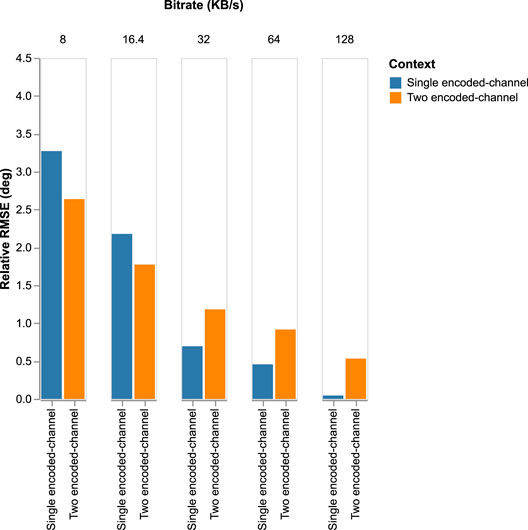
FIGURE 14. Relative RMSE degradation for a varying bitrate performed for the two models: 1) Single encoded-channel model where one of the channels is without compression and the second is encoded with EVS and the internal delay has been compensated. 2) The two encoded-channel model where the two inputs are encoded similarly with EVS at a varying bitrate.

FIGURE 15

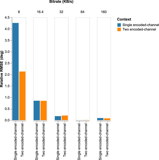
FIGURE 15. Relative RMSE degradation for a varying bitrate performed for the two models: 1) Single encoded-channel model where one of the channels is without compression and the second is encoded with PyAWNeS. 2) The two encoded-channel model where the two inputs are encoded similarly with PyAWNeS at a varying bitrate.

FIGURE 16

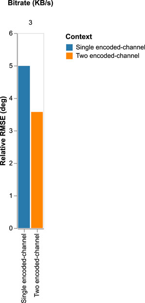
FIGURE 16. Relative RMSE degradation for a varying bitrate performed for the two models: 1) Single encoded-channel model where one of the channels is without compression and the second is encoded with Lyra. 2) The two encoded-channel model where the two inputs are encoded similarly with Lyra at a varying bitrate.

5.5 Varying Codecs for the Two Channels With an Equal Bitrate

As it was proven that a trained (w/PyAWNeS@16.4) model could overcome degradation at a low bitrate, then it could be beneficial for challenging the condition where we have a variance in codecs among the two channels with a similar fixed bitrate of 16.4 kB/s. For this experiment, we generate different test sets in which we select different codecs for the two channels. To investigate the variance of the codecs’ impact, we consider matching the condition where the two channels are encoded with PyAWNeS as our baseline. Our results are shown in Table 4. The model is not as good as the baseline matched training. The degradation can be attributed to the loss of information in encoding in the second channel when using EVS or Opus. This degradation is more pronounced when the two channels are different from the training set, with more than 25% misclassified estimation. It’s interesting to note that even if we employ PyAWNeS for one of the two channels, the model is still more efficient when the two channels are encoded similarly. We see a 38% degradation in RMSE when the audio inputs are similarly encoded with EVS at 16.4 kB/s (Table 2) versus 46 % and 100% when one of the channels is encoded with PyAWNeS, and Opus respectively (Table 4). This can be explained by the mismatch in the training and test data. This degradation can be recovered if the training sample presented to the model (w/Random@16.4) are encoded with a randomly selected codec at 16.4 kB/s. A more accurate estimation could be noticed when at least one of the two channels are encoded with PyAWNeS.

TABLE 4

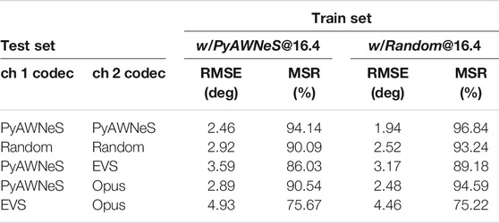
TABLE 4. Performance of models: trained with PyAWNeS at 16.4 kB/s (w/PyAWNeS@16.4), and trained on randomly selected codec (w/Random@16.4) on varying codecs input at the same bitrate (16.4 kB/s).

6 Conclusion and Outlook

The current study investigated the effect of speech compression on a DNN-based DoA classifier model. We analyzed the degradation of a target DoA estimation as a function of bitrates available for the input audio. The experiments included different types of codecs. It was intuitively expected that at lower bit rates the distortion is higher, leading to the removal of some information about speaker location, and to a lower DoA accuracy. In contrast, codecs with higher bit rates introduce less distortion and therefore could be expected to provide higher DoA accuracy. As the spectral information has a high impact on the performance of our DoA classifier, it was demonstrated that PyAWNeS is more suitable than EVS and Opus to train the model at a low bitrate as it preserves location information better. We also showed that training the DoA classifier with PyAWNeS at 16.4 kB/s can outperform the raw data-based model and recover degradation for the two similarly encoded channels. We further demonstrated that for almost all codecs, when limited bandwidth is available, a two encoded-channel input over a single channel input scenario is preferable. However, for the best performance, it is optimal to encode one channel with the highest bitrate, given raw data for the second channel. This achievement opens up another experiment where different devices may not support the same codec. For that, a trained model on a randomly selected codec for both channels at 16.4 kB/s likely approves previous results by highlighting higher accuracy gain when at least one of the two channels are encoded with PyAWNeS. This can be especially useful with a multi-channel scenario so that the model can leverage the optimal devices’ selection for the localization task. Our results thus demonstrate that while coding does degrade DoA performance, with a suitable choice of codec and training of the DoA-estimator, the reduction in accuracy remains reasonable. DoA estimation is thus viable also for encoded signals.

Data Availability Statement

Reproducible results are available on https://gitlab.com/speech-interaction-technology-aalto-university/results-speech-localization.

Author Contributions

MM: Conceptualization, investigation, methodology, development, results and writing—original draft. PZ: Conceptualization, methodology, and development. TB: Methodology, resources, writing—review and editing. ZL: Supervision. All authors contributed to the article and approved the submitted version.

Conflict of Interest

The authors declare that the research was conducted in the absence of any commercial or financial relationships that could be construed as a potential conflict of interest.

Publisher’s Note

All claims expressed in this article are solely those of the authors and do not necessarily represent those of their affiliated organizations, or those of the publisher, the editors and the reviewers. Any product that may be evaluated in this article, or claim that may be made by its manufacturer, is not guaranteed or endorsed by the publisher.

References

Bäckström, T., Mariem, B. M., Zarazaga, P. P., Ranjit, M., Das, S., and Lachiri, Z. (2021). “PyAWNeS-Codec: Speech and Audio Codec for Ad-Hoc Acoustic Wireless Sensor Networks,” in 2021 29th European Signal Processing Conference (EUSIPCO), Dublin, Ireland, August 2021. doi:10.23919/eusipco54536.2021.9616344

CrossRef Full Text | Google Scholar

Bäckström, T. (2017). Speech Coding with Code-Excited Linear Prediction. Part of: Signals and Communication Technology. Springer.

Google Scholar

Bengio, Y., Lamblin, P., Popovici, D., and Larochelle, H. (2007). Greedy Layerwise Training of Deep Networks. Adv. Neural Inf. Process. Syst. 19, 153.

Google Scholar

Bengio, Y., Courville, A., and Vincent, P. (2013). Representation Learning: A Review and New Perspectives. IEEE Trans. Pattern Anal. Mach. Intell. 35, 1798–1828. doi:10.1109/tpami.2013.50

PubMed Abstract | CrossRef Full Text | Google Scholar

Bruhn, S., Eksler, V., Fuchs, G., and Gibbs, J. (2012). “Codec for Enhanced Voice Services (Evs)-The New 3gpp Codec for Communication,” in Workshop at the 140th AES Convention 2016, Paris, June 4–7.

Google Scholar

Chakrabarty, S., and Habets, E. A. P. (2017). “Broadband Doa Estimation Using Convolutional Neural Networks Trained with Noise Signals,” in IEEE Workshop on Applications of Signal Processing to Audio and Acoustics (WASPAA), New Paltz, NY, October 2017, 136–140. doi:10.1109/waspaa.2017.8170010

CrossRef Full Text | Google Scholar

Chen, X., Wang, D., Y, J. X., and Wu, Y. (2018). A Direct Position-Determination Approach for Multiple Sources Based on Neural Network Computation. Sensors 18, 1925. doi:10.3390/s18061925

PubMed Abstract | CrossRef Full Text | Google Scholar

Cobos, M., Antonacci, F., Alexandridis, A., Mouchtaris, A., and Lee, B. (2017). A Survey of Sound Source Localization Methods in Wireless Acoustic Sensor Networks. Wireless Commun. Mobile Comput. 2017, 1–24. doi:10.1155/2017/3956282

CrossRef Full Text | Google Scholar

Dean, J., Corrado, G., Monga, R., Chen, K., Mao, M. D. M., Le, Q. V., et al. (2012). Large Scale Distributed Deep Networks. Adv. Neural Inf. Process. Syst. 1, 1223–1231.

Google Scholar

Garcia, N., Vasquez-Correa, J., Arias-Londono, J., Várgas-Bonilla, J ., and Orozco -Arroyave, J . (2015). “Automatic Emotion Recognition in Compressed Speech Using Acoustic and Non -linearfeatures,” in 20th Symposium on Signal Processing, Images and Computer Vision ( STSIVA), Bogotá, September 2015. doi:10.1109/stsiva.2015.7330399

CrossRef Full Text | Google Scholar

Huang, H. J., Yang, J., Huang, H., Song, Y. W., and Gui, G. (2018). Deep Learning for Super-resolution Channel Estimation and Doa Estimation Based Massive Mimo System. IEEE Trans. Veh. Technol. 3, 8549–8560. doi:10.1109/tvt.2018.2851783

CrossRef Full Text | Google Scholar

Kleijn, W. B., Storus, A., Chinen, M., Denton, T., Lim, F. S. C., Luebs, A., et al. (2021). Generative Speech Coding with Predictive Variance Regularization. arXiv. arXiv:2102.09660.

Google Scholar

Liu, D. C., and Nocedal, J. (1989). On the Limited Memory Bfgs Method for Large Scale Optimization. Math. Program. 45, 503–528. doi:10.1007/bf01589116

CrossRef Full Text | Google Scholar

Liu, Z. M., Zhang, C. W., and Philip, S. Y. (2018). Direction-of-arrival Estimation Based on Deep Neural Networks with Robustness to Array Imperfections. IEEE Trans. Antennas Propag. 66, 7315–7327. doi:10.1109/tap.2018.2874430

CrossRef Full Text | Google Scholar

Liu, W. (2020). Super Resolution Doa Estimation Based on Deep Neural Network. Sci. Rep. 10, 19859. doi:10.1038/s41598-020-76608-y

PubMed Abstract | CrossRef Full Text | Google Scholar

Mac, K.-N. C., Xiaodong, C., Zhang, W., and Picheny, M. (2019). Large-scale Mixed-Bandwidth Deep Neural Network Acoustic Modeling for Automatic Speech Recognition. arXiv. arXiv preprint arXiv:1907.04887.

Google Scholar

Panayotov, V., Chen, G., Povey, D., and Khudanpur, S. (2015). “Librispeech: an ASR Corpus Based on Public Domain Audio Books,” in 2015 IEEE International Conference on Acoustics, Speech and Signal Processing (ICASSP), South Brisbane, Queensland, April, 2015, 5206–5210. doi:10.1109/icassp.2015.7178964

CrossRef Full Text | Google Scholar

Pertilä, P., and Parviainen, M. (2019). “Time Difference of Arrival Estimation of Speech Signals Using Deep Neural Networks with Integrated Time-Frequency Masking,” in ICASSP 2019 - 2019 IEEE International Conference on Acoustics, Speech and Signal Processing (ICASSP), Brighton, May 2019, 436–440. doi:10.1109/icassp.2019.8682574

CrossRef Full Text | Google Scholar

Rämö, A., and Toukomaa, H. (2015). “Subjective Quality Evaluation of the 3gpp Evs Codec,” in 2015 IEEE International Conference on Acoustics, Speech and Signal Processing (ICASSP), South Brisbane, Queensland, April 2015 (IEEE), 5157–5161. doi:10.1109/icassp.2015.7178954

CrossRef Full Text | Google Scholar

Scheibler, R., Bezzam, E., and Dokmanic, I. (2017). “Pyroomacoustics: A python Package for Audio Room Simulations and Array Processing Algorithms,” in Proceedings 2018 IEEE International Conference on Acoustics, Speech and Signal Processing (ICASSP), Calgary, AB, Canada, April, 2018. doi:10.1109/ICASSP.2018.8461310

CrossRef Full Text | Google Scholar

Shehadeh, H. A., Idris, M. Y. I., Ahmedy, I., Ramli, R., and Noor, N. M. (2018). The Multi-Objective Optimization Algorithm Based on Sperm Fertilization Procedure (Mosfp) Method for Solving Wireless Sensor Networks Optimization Problems in Smart Grid Applications. Energies 11. doi:10.3390/en11010097

CrossRef Full Text | Google Scholar

Siegert, I., Lotz, A. F., Maruschke, M., Jokisch, O., and Wendemuth, A. (2016). “Emotion Intelligibility within Codec-Compressed and Reduced Bandwidth Speech,” in Speech Communication; 12. ITG Symposium, Paderborn, Germany, October, 2016 (VDE), 1–5.

Google Scholar

Takeda, R., and Komatani, K. (2016). “Multiple Sound Source Localization Based on Deep Neural Networks Using Independent Location Model,” in 2016 IEEE Spoken Language Technology Workshop (SLT), San Juan, December 2016, 603–609.

Google Scholar

The Cisco Visual Networking Index (2020). Global mobile Data Traffic Forecast Update, 2017-2022. Hershey, PA, USA: IGI Global.

Google Scholar

Valin, J. M., Vos, K., and Terriberry, T. (2012). Definition of the Opus Audio Codec. IETF, 1–326.

Google Scholar

Xiao, X., Zhao, S., Zhong, X., Jones, D. L., Chng, E. S., and Li, H. (2015). “A Learning-Based Approach to Direction of Arrival Estimation in Noisy and Reverberant Environments,” in IEEE International Conference on Acoustics, Speech and Signal Processing (ICASSP), South Brisbane, April 2015, 2814–2818. doi:10.1109/icassp.2015.7178484

CrossRef Full Text | Google Scholar

Yang, C., and Li, J. (2016). Interference Mitigation and Energy Management in 5g Heterogeneous Cellular Networks. Hershey, PA, USA: IGI Global.

Google Scholar

Yu, D., and Deng, L. (2011). Deep Learning and its Applications to Signal and Information Processing [Exploratory DSP. IEEE Signal. Process. Mag. 28, 145–154. doi:10.1109/msp.2010.939038

CrossRef Full Text | Google Scholar

Zarazaga, P. P., Bäckström, T., and Sigg, S. (2020). Acoustic Fingerprints for Access Management in Ad-Hoc Sensor Networks. IEEE Access 8, 166083–166094. doi:10.1109/access.2020.3022618

CrossRef Full Text | Google Scholar

Zarazaga, P. P., Mansali, M. B., Bäckström, T., and Lachiri, Z. (2021). “Cancellation of Local Competing Speaker with Near-Field Localizationfor Distributed Ad-Hoc Sensor Network,” in Interspeech 2021, Brno, September 2021, 676–680. doi:10.21437/interspeech.2021-1329

CrossRef Full Text | Google Scholar