EKF- and UKF-Based Estimators for Radar System

In radar, the measurements (like the range and radial velocity) are determined from the time delay and Doppler shift. Since the time delay and Doppler shift are estimated from the phase of the received echo, the concerned estimation problem is nonlinear. Consequently, the conventional estimator based on the fast Fourier transform (FFT) is prone to yield high estimation errors. Recently, nonlinear estimators based on kernel least mean square (KLMS) are introduced and found to outperform the conventional estimator. However, estimators based on KLMS are susceptible to incorrect choice of various system parameters. Thus, to mitigate the limitation of existing estimators, in this paper, two efficient low-complexity nonlinear estimators, namely, the extended Kalman filter (EKF) and the unscented Kalman filter (UKF), are proposed. The EKF is advantageous due to its implementation simplicity; however, it suffers from the poor representation of the nonlinear functions by the first-order linearization, whereas UKF outperforms the EKF and offers better stability due to exact consideration of the system nonlinearity. Simulation results reveal improved accuracy achieved by the proposed EKF- and UKF-based estimators.

1 Introduction

Radar systems are generally used in applications like target identification and tracking, air traffic control, and remote sensing (Richards, 2005). In radar systems, a signal burst is transmitted by the transmitter, and the receiver receives a scattered form of this signal in return. This scattering is quantified with time delay and Doppler shift in the received signal, which gives measures on the range and radial velocity of the target. The range and radial velocity of the target are used as measurements in radar applications (Richards et al., 2010). Thus, an appropriate estimation of time delay and Doppler shift is required for accurate tracking of the target trajectory. Some of the major developments in estimating these parameters are introduced in the literature by Abatzoglou and Gheen (1998), Li and Wu (1998), and Yang et al. (2011). Abatzoglou and Gheen (1998) introduced an approximate maximum likelihood estimator based on the fast Fourier transform (FFT) for estimating the desired time delay and Doppler shift. In the study by Li and Wu (1998), a nonconvex least square cost function was defined in terms of the desired parameters. Thereafter, the estimation problem reduces to the minimization of the cost function. In a later development, Yang et al. (2011) introduced a multiple signal classification technique commonly known as MUSIC and estimated the desired time delay and Doppler shift by solving the problem of spectral estimation.

The existing approaches introduced in the literature by Abatzoglou and Gheen (1998), Li and Wu (1998), and Yang et al. (2011) suffer from poor estimation accuracy, especially in low signal-to-noise ratio (SNR) conditions (often the case with practical radar systems). In the literature, this phenomenon has been termed as the SNR thresholding effect (Abatzoglou and Gheen; Rife and Boorstyn, 1974; Kay, 1993; Kay, 1998). The desired parameters to be estimated are contained in the phase of received echo. Consequently, the parameter estimation problem in a radar system is nonlinear (Richards, 2005; Richards et al., 2010). Therefore, as a recent solution for efficient estimation of time delay and Doppler shift, a kernel least mean square (KLMS)–based nonlinear estimator has been introduced by Singh et al. (2017) and Singh et al. (2019). The KLMS-based estimator uses representer theorem (Liu et al., 2011) to recursively estimate the nonlinearity (between the unknown parameters and returning signal) in a reproducing kernel Hilbert’s space (RKHS) (Liu et al., 2011, 2008). The estimated parameters are adaptively updated using the least mean square algorithm (Liu et al., 2011) in RKHS. However, a major drawback in the KLMS-based algorithm is that they require precise knowledge of various system parameters, like the kernel width, step size, and dictionary thresholds. Suitable values of these parameters are obtained by running their values in a fixed range. Moreover, these parameter values are model specific (Liu et al., 2008; Mitra and Bhatia, 2014;Mitra and Bhatia, 2017); hence, a priori fixed set of parameter values are not appropriate for targets with varying system dynamics (e.g., varying range and radial velocity) which is most common in practical problems. Consequently, the KLMS-based estimators offer poor estimation accuracy. Another drawback is that, being a stochastic gradient-based algorithm, the KLMS-based estimators require a large number of iterations to converge to a minimum error (between the desired and estimated parameters) solution (Liu et al., 2011).

This paper introduces two novel nonlinear estimation techniques to counter drawbacks of estimators in the literature and improve the estimation of time delay and Doppler shift. The proposed estimation techniques are based on two popular nonlinear estimators: the extended Kalman filter (EKF) (Bar-Shalom et al., 2004) and the unscented Kalman filter (UKF) (Julier et al., 2000; Julier and Uhlmann, 1997; Julier and Uhlman, 2004). To the best of the authors’ knowledge, the EKF and UKF have been tested for target tracking using radar-based measurements (Cortina et al., 1991; Farina et al., 2002; Kulikov and Kulikova, 2015). The other version of Kalman filter, modified convolution kernel function (MCKF) (Gu et al., 2019), has been used for parameter estimation of returning signal (model as linear frequency modulated (LFM) signal) in the specific application of synthetic aperture radar. However, the EKF and UKF have not been explored for estimating the time delay and Doppler shift for target tracking. The EKF implements a basic Kalman filter (Bar-Shalom et al., 2004) and offers a simple implementation. However, it approximates the nonlinear system as a linear model obtained by the first-order linearization. Subsequently, it suffers from poor accuracy and stability, especially in a complex environment such as low SNR and heavy-tailed clutter. Poor accuracy in estimating the target’s states causes ambiguity in target identification. Unlike EKF, UKF considers the system models in their original nonlinear form, which is beneficial in accurate estimation of a target’s parameters in a complex environment. Accuracy of the proposed estimation techniques based on EKF and UKF is compared with the existing KLMS-based estimator (called KLMS-Modified NC) and conventional estimator based on FFT. Simulation results reveal a lower normalized mean square error (NMSE) and variance for the proposed estimators.

The main purpose for which radars are commonly used is detection and tracking. Usually, in a radar system, the tracking is followed by the detection and estimation of parameters such as range, radial velocity, and angle. The estimated range, radial velocity, and angle are used as measurements for the tracker. In the proposed work, we are estimating the target range (time delay) and radial velocity (Doppler shift) at the signal level before detection. Therefore, the estimated parameters can be supplied directly to the tracker for tracking; in the literature, this technique is notably known as track before detection (TBD) (Buzzi et al., 2008; Kwon et al., 2019). Consequently, as TBD finds application in stressful environments (heavily perturbed by clutter) like marine, vehicles in traffic, and ground with complex terrains, with the assumption of known angle information, our proposed estimation approach provides improved measurements for tracker in such applications.

The rest of the paper is organized as follows: Section 2 describes the signal model for received radar return for the transmitted LFM signal. The proposed EKF- and UKF-based estimators are described in Section 3. Simulation results along with analytical expressions for CRLB on the variance in estimating time delay and Doppler shift are discussed in Section 4. Finally, Section 5 concludes the contribution of this work.

Notations. Scalar variables (constants) are denoted by lower (upper) case letters. Vectors (matrices) are denoted by boldface lower (upper) case letters. Superscripts ${(\cdot )}^T$, ${(\cdot )}^H$, and ${(\cdot )}^{\text{*}}$ denote matrix transpose, matrix complex conjugate transpose, and scalar complex conjugate operation, respectively. $\mathbb{E}[\cdot ]$ denotes statistical expectation. $\mathrm{ℂ}$ and $\mathrm{ℝ}$ denote a set of complex and real numbers, respectively. $\mathrm{\Re }(\cdot )$ and $\mathrm{\Im }(\cdot )$ denote the real and imaginary part of the complex number, respectively.

2 Signal Model Formulation

In this section, we derive the radar return signal model, which describes the relationship between the radar return and the desired unknown parameters, namely, the time delay and the Doppler shift. We choose the most commonly used radar system called the monostatic LFM radar (Levanon and Mozeson, 2004; Richards et al., 2010) with an assumption that the platform holding a radar system is static. Block diagram of the considered monostatic radar is presented in Figure 1. As shown in Figure 1, the radar transmitter generates a burst of LFM pulses at a baseband frequency (a sample baseband LFM signal is shown in Figure 2), where LFM pulses are separated by a fixed duration called pulse repetition interval (PRI). For transmission, the pulse burst is modulated with high-frequency carrier signal, resulting in a broadband LFM signal (a sample broadband LFM signal is presented in Figure 3). The on-board receiver captures a scattered form of transmitted signal returning from the target. Subsequently, the received signal is degenerated to a scattered form of the originally transmitted signal. Scattering is introduced due to two factors: i) time delay due to to-and-from propagation of signal between the antenna and the target and ii) Doppler shift introduced due to target’s radial velocity. A sample scattered signal is shown in Figure 4¹.

FIGURE 1

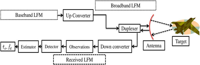
FIGURE 1. Block diagram of the radar system model, depicting the transmission of signal and processing of scattered signal to estimate the target’s unknown parameters: time delay and Doppler shift.

FIGURE 2

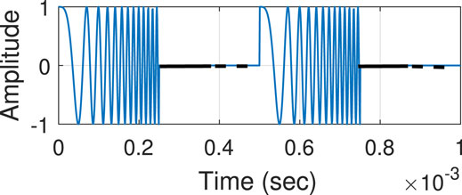
FIGURE 2. Baseband LFM at low frequency.

FIGURE 3

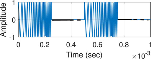
FIGURE 3. Broadband LFM at carrier frequency.

FIGURE 4

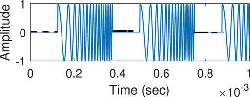
FIGURE 4. Received LFM signal (time-delayed and Doppler-shifted version of baseband LFM).

The LFM baseband signal is denoted by $s_{\text{LFM}}\left(t\right)$, i.e.,

$s_{\text{ LFM}}\left(t\right)=\{\begin{array}{cc}a\exp \left(j\pi \gamma t^2\right)\text{;}& 0\le t\le T_o\\ 0\text{;}& T_o<t\le T_{\text{PRI}},\end{array}$

where a is the amplitude, γ is the frequency sweep rate, $T_o$ is the pulse duration, and $T_{\text{PRI}}$ is the PRI. Note that the frequency of $s_{\text{ LFM}}\left(t\right)$ is time-varying with instantaneous frequency being $fi\left(t\right)$²$=\mathrm{\gamma }t$.

The $m^{th}$ pulse in the burst of M LFM pulses can be represented as the time-shifted form of $s_{\text{ LFM}}\left(t\right)$, i.e.,

$s_m\left(t\right)=s_{\text{LFM}}\left(t-m{T}_{\text{PRI}}\right)\mathrm{for}0\le t\le T_o,(1)$

where $m\in \left[\mathrm{0,1},\dots ,M-1\right]$, with M being the total number of pulses in the pulse burst.

As discussed earlier, $s_m\left(t\right)$ is modulated with high-frequency carrier signal. The modulated signal can be represented as

$s\left(t\right)=\left\{s_m\left(t\right)\right\}\exp \left(j2\pi f_{c}t\right)\text{,}(2)$

where $f_c$ is the frequency of the carrier signal.

The returning signal $r_m\left(t\right)$ is a time-delayed variant of $s\left(t\right)$. If ${\tau }_m$ is the time delay in the $m^{th}$ pulse, then

${\tau }_m={\tau }_o-\frac{2}{c}\left\{vm{T}_{\text{PRI}}\right\},(3)$

where ${\tau }_o$ is the time delay in the first pulse, v is the target radial velocity, and c is the velocity of light. Without loss of generality, for the time on target, i.e., for M pulses, v is assumed to be constant; thereby, constant Doppler shift is assumed. The time difference $\frac{2}{c}\left\{vm{T}_{\text{PRI}}\right\}$ is the time shift in the return signal due to the change in position of the target over $m{T}_{\text{PRI}}$. Subsequently, $r_m\left(t\right)$ is

$r_m\left(t\right)=\left\{s_m\left(t-{\tau }_m\right)\right\}\text{exp}\left(j2\pi f_c\left(t-{\tau }_m\right)\right)+w_m\left(t\right),(4)$

where $w_m\left(t\right)$ is the additive thermal noise process.

The returning signal, $r_m\left(t\right)$, in the baseband can be written as

$r_m\left(t\right)=\left\{s_m\left(t-{\tau }_m\right)\right\}\text{exp}\left(-j2\pi f_c{\tau }_m\right)+w_m\left(t\right).(5)$

Substituting $s_m\left(t\right)$ from Eq. 1, we get

$r_m\left(t\right)=s_{\text{LFM}}\left(t-m{T}_{\text{PRI}}-{\tau }_m\right)\text{exp}\left(-j2\pi f_c{\tau }_m\right)+w_m\left(t\right).(6)$

The matched filter output is given by

$r_m\left(t\right)={\displaystyle {\int }_{{\tau }_m}^{{\tau }_m+T_o}{s}_{\text{LFM}}\left(t-m{T}_{\text{PRI}}-{\tau }_m\right)s_{\text{LFM}}^{\text{*}}\left(t-m{T}_{\text{PRI}}-\tau \right)\times \text{exp}\left(-j2\pi f_c{\tau }_m\right)dt+w_m\left(t\right)}.(7)$

Next, taking the Fourier transform yields

$\begin{array}{c}{R}_m\left(f\right)=\text{exp}\left(-j2\pi f_c{\tau }_m\right){\displaystyle \int {\displaystyle {\int }_{{\tau }_m}^{{\tau }_m+T_o}{s}_{\text{LFM}}\left(t-m{T}_{\text{PRI}}-{\tau }_m\right)s_{\text{LFM}}^{\text{*}}\left(t-m{T}_{\text{PRI}}-\tau \right)\text{exp}\left(-j2\pi f\tau \right)dtd\tau }}\\ +w_m\left(f\right).\\ =\text{exp}\left(-j2\pi f_c{\tau }_m\right){\displaystyle \int {\displaystyle {\int }_{{\tau }_m}^{{\tau }_m+T_o}{s}_{\text{LFM}}\left(t-m{T}_{\text{PRI}}-{\tau }_m\right)s_{\text{LFM}}^{\text{*}}\left(t-m{T}_{\text{PRI}}-\tau \right)}}\\ \times \text{exp}\left(-j2\pi f\left(m{T}_{\text{PRI}}+\tau -t\right)\right)\text{exp}\left(-j2\pi f\left(t-m{T}_{\text{PRI}}\right)\right)dtd\tau +w_m\left(f\right).\\ =\text{exp}\left(-j2\pi f_c{\tau }_m\right){\displaystyle {\int }_{{\tau }_m}^{{\tau }_m+T_o}{s}_{\text{LFM}}\left(t-m{T}_{\text{PRI}}-{\tau }_m\right)\text{exp}(-j2\pi f\left(t-m{T}_{\text{PRI}}-{\tau }_m\right)dt\text{exp}\left(-j2\pi f{\tau }_m\right)}\\ \times {\displaystyle \int s_{\text{LFM}}^{\text{*}}\left(t-m{T}_{\text{PRI}}-\tau \right)\text{exp}\left(-j2\pi f\left(m{T}_{\text{PRI}}+\tau -t\right)\right)\times d\tau +w_m\left(f\right)}.\end{array}$

Thus, $R_m\left(f\right)$ can be written as

$R_m\left(f\right)={\left|S_{\text{ LFM}}\left(f\right)\right|}^2\text{exp}\left(-j2\pi f_c{\tau }_m\right)\text{exp}\left(-j2\pi f{\tau }_m\right)+w_m\left(f\right).$

Here, $S_{\text{ LFM}}\left(f\right)$ is the Fourier transform of $s_{\text{ LFM}}\left(t\right)$.

Sampling in the frequency domain at $l=[\mathrm{0,1},\dots ,L-1]$ with an interval of $\text{Δ}f$ and dividing by $|S_{\text{ LFM}}\left(l\text{Δ}f\right){|}^2$ yield

$r\left(m,l\right)=\text{exp}\left(-j2\pi f_c{\tau }_m\right)\text{exp}\left(-j2\pi l\text{Δ}f{\tau }_m\right)+w\left(m,l\right),(8)$

where $w\left(m,l\right)$ is the discrete sample of the thermal noise process.

Substituting ${\tau }_m$ from Eq. 3, we get

$r\left(m,l\right)=\text{exp}\left(j2\pi m{f}_d{T}_{\text{PRI}}\right)\text{exp}\left(-j2\pi l\text{Δ}f{\tau }_o\right)\text{exp}\left(j2\pi f_{d}ml\left(\frac{T_{\text{PRI}}\text{Δ}f}{f_c}\right)\right)+w\left(m,l\right),(9)$

where $f_d=2v{f}_c/c$ is the unknown Doppler shift due to the target’s radial velocity.

From Eq. 9, it is explicit that the returning signal, $r\left(m,l\right)$, is exponentially nonlinearly related to the desired time delay, ${\tau }_o$, and Doppler shift, $f_d$. The adaptive estimators to estimate ${\tau }_o$ and $f_d$ based on KLMS-Modified NC exploiting nonlinearity were proposed by Singh et al. (2017) and Singh et al. (2019). However, the performance of the KLMS-Modified NC-based estimator is susceptible to inappropriate values of various system parameters. Moreover, being an adaptive algorithm, KLMS-Modified NC requires a large number of iterations to reach the theoretical optimum solution, leading to a large running time. In this paper, to mitigate the shortcomings of the existing state-of-the-art algorithms, we introduce two advanced estimation techniques based on EKF and UKF for estimating ${\tau }_o$ and $f_d$ from the returning signal $r\left(m,l\right)$.

3 Estimation of Time Delay and Doppler Shift

In this section, the proposed EKF- and UKF-based estimators for ${\tau }_o$ and $f_d$ are described in detail. In noisy environments (as the considered radar system), Bayesian framework-based estimators are applied for several decades (refer to Bar-Shalom et al., 2004; Anderson and Moore, 2012; and Brown and Hwang, 1992 for a detailed discussion). The Bayesian framework is based on the state-space formulation (discussed in Section 3.1) (Bar-Shalom et al., 2004) of the system model, and it is implemented in two steps: prediction and update. Two popular simplifications of the Bayesian framework are Gaussian filtering (Bar-Shalom et al., 2004) and particle filtering (Arulampalam et al., 2002). The Gaussian filters are preferred over particle filters due to sufficiently high estimation accuracy at an appreciably low computational cost. The proposed EKF and UKF for ${\tau }_o$ and $f_d$ estimation are two popular Gaussian filters. We, first, formulate the state-space model for the LFM radar system and briefly discuss the Bayesian framework. After that, we elaborate the proposed EKF- and UKF-based estimation of ${\tau }_o$ and $f_d$.

3.1 State-Space Model for Radar Systems

The state-space model consists of state and measurement models, where the state model characterizes the state dynamics while the measurement model represents the mathematical relation between the state and measurement. Note that the state is defined with the unknown desired parameters (${\tau }_o$ and $f_d$ in this case), while the measurement consists of the observed quantities (the returning signal $r\left(m,l\right)$). Subsequently, the state and the measurement variables are formulated as $\mathbf{x}={\left[{\tau }_o{f}_d\right]}^T$ and $\mathbf{y}={\left[\mathrm{\Re }\left(r\left(m,l\right)\right)\mathrm{\Im }\left(r\left(m,l\right)\right)\right]}^T$, respectively. In Eq. 9, the state-space model is formulated with a constant increase in the time delay over the sampling interval due to the constant radial velocity assumption. Any error due to this assumption is considered as the process noise. Similarly, the constant radial velocity assumption gives constant Doppler shift over time and the practical variation is again considered as the process noise. Subsequently, the state model is formulated as

${\mathbf{x}}_{k+1}=f\left(x_k\right)+{\mathrm{\eta }}_k={\mathbf{x}}_k+\Delta \mathrm{x}+{\mathrm{\eta }}_k,(10)$

where $k\in \left\{\mathrm{1,2},\cdots ,K\right\}$, $K=ML$ is the total number of discretized samples of returning signal, and $\text{Δ}\mathbf{x}=\left[\frac{T_o}{K},0\right]$ is a constant shift in $\mathbf{x}$ between successive samples of returning signal. ${\eta }_k$ is additive process noise, compensating for modeling errors.

Following Eq. 9, the measurement model $\left({\mathbf{y}}_{k+1}\right)$ is formulated as

${\mathrm{y}}_{k+1}=h\left({\mathbf{x}}_{k+1}\right)+{\mathrm{v}}_{k+1}=\left[\begin{array}{c}\mathrm{\Re }\left(\text{exp}\left(j2\pi m{\mathbf{x}}_{k+1}\left(2\right)T_{\text{PRI}}\right)\text{exp}\left(-j2\pi l\text{Δ}f{\mathbf{x}}_{k+1}\left(1\right)\right)\text{exp}\left(j2\pi {\mathbf{x}}_{k+1}\left(2\right)ml\left(\frac{T_{\text{ PRI}}\text{Δ}f}{f_c}\right)\right)\right)\\ \mathrm{\Im }\left(\text{exp}\left(j2\pi m{\mathbf{x}}_{k+1}\left(2\right)T_{\text{PRI}}\right)\text{exp}\left(-j2\pi l\text{Δ}f{\mathbf{x}}_{k+1}\left(1\right)\right)\text{exp}\left(j2\pi {\mathbf{x}}_{k+1}\left(2\right)ml\left(\frac{T_{\text{PRI}}\text{Δ}f}{f_c}\right)\right)\right)\end{array}\right]+{\mathrm{v}}_{k+1},(11)$

where ${\mathbf{v}}_k$ represents measurement noise. It should be mentioned that the measurement noise compensates for the error in capturing and/or processing of returning signals. In the Gaussian filtering, ${\mathbf{\eta }}_k$ and ${\mathbf{v}}_k$ are assumed to be zero-mean Gaussian with covariances ${\mathbf{Q}}_k$ and ${\mathbf{R}}_k$, respectively. Also, we adopt the standard modeling strategy from the filtering literature and consider the noises (process and measurement) to have additive effects.

3.2 Bayesian Framework for Filtering

The Bayesian filtering is performed in two steps.

3.2.1 Prediction

This step constructs the probability distribution function (pdf) of states one step forward in time (in reference to the available measurements) using the Chapman–Kolmogorov equation (Bar-Shalom et al., 2004; Anderson and Moore, 2012), i.e.,

$P\left({\mathbf{x}}_k|{\mathbf{y}}_{1:k-1}\right)={\displaystyle \int P\left({\mathbf{x}}_k|{\mathbf{x}}_{k-1}\right)P\left({\mathbf{x}}_{k-1}|{\mathbf{y}}_{1:k-1}\right)d{\mathbf{x}}_{k-1}},(12)$

where $P(\cdot )$ represents the pdf. $P\left({\mathbf{x}}_k|{\mathbf{y}}_{1:k-1}\right)$ is commonly known as prior pdf.

3.2.2 Update

This step reconstructs the pdf $P\left({\mathbf{x}}_k|{\mathbf{y}}_{1:k-1}\right)$ on the receipt of a new measurement ${\mathbf{y}}_k$ using the Bayes rule (Bar-Shalom et al., 2004; Anderson and Moore, 2012), i.e.,

$P\left({\mathbf{x}}_k|{\mathbf{y}}_{1:k}\right)=P\left({\mathbf{x}}_k|{\mathbf{y}}_{1:k-1},{\mathbf{y}}_k\right)=\frac{1}{c_k}P\left({\mathbf{y}}_k|{\mathbf{x}}_k\right)P\left({\mathbf{x}}_k|{\mathbf{y}}_{1:k-1}\right),(13)$

where $P\left({\mathbf{y}}_k|{\mathbf{x}}_k\right)$ is the measurement likelihood which is obtained from Eq. 11 and $c_k$ is a normalization constant, i.e.,

$c_k=P\left({\mathbf{y}}_k|{\mathbf{y}}_{1:k-1}\right)={\displaystyle \int P\left({\mathbf{y}}_k|{\mathbf{x}}_k\right)P\left({\mathbf{x}}_k|{\mathbf{y}}_{1:k-1}\right)d{\mathbf{x}}_k}.(14)$

The objective of Bayesian filtering is to construct $P\left({\mathbf{x}}_k|{\mathbf{y}}_{1:k}\right)$, which is popularly known as posterior pdf.

Hereafter, we denote $P\left({\mathbf{x}}_k|{\mathbf{y}}_{1:k-1}\right)\sim P\left({\mathbf{x}}_{k|k-1}\right)$ and $P\left({\mathbf{x}}_k|{\mathbf{y}}_{1:k}\right)\sim P\left({\mathbf{x}}_{k|k}\right)$, which are standard notations used in estimation and filtering literature (Brown et al., 1992; Bar-Shalom et al., 2004; Anderson and Moore, 2012).

3.3 EKF-Based Estimation of ${\tau }_o$ and $f_d$

From the state-space model of the considered radar systems (Eqs. 10, 11), the estimation of ${\tau }_o$ and $f_d$ from returning signal, $r\left(m,l\right)$, is simplified as an estimation problem of ${\mathbf{x}}_k$ from known measurement ${\mathbf{y}}_k$. The EKF is an analytical simplification of the above-discussed Bayesian framework. It assumes the conditional pdfs in the Bayesian framework (Eqs. 12–14) as Gaussian, i.e.,

$P\left({\mathbf{x}}_{k|k-1}\right)\sim \mathcal{N}\left({\mathbf{x}}_{k|k-1};{\widehat{\mathbf{x}}}_{k|k-1},{\mathbf{P}}_{k|k-1}\right),(15)$

$P\left({\mathbf{x}}_{k|k}\right)\sim \mathcal{N}\left({\mathbf{x}}_{k|k};{\widehat{\mathbf{x}}}_{k|k},{\mathbf{P}}_{k|k}\right),(16)$

where $\mathcal{N}$ denotes real Gaussian distribution, ${\widehat{\mathbf{x}}}_{k|k-1}$ and ${\mathbf{P}}_{k|k-1}$ are mean and covariance of ${\mathbf{x}}_{k|k-1}$, and ${\widehat{\mathbf{x}}}_{k|k}$ and ${\mathbf{P}}_{k|k}$ are mean and covariance of ${\mathbf{x}}_{k|k}$. Subsequently, the problem is further simplified to determine ${\widehat{\mathbf{x}}}_{k|k-1}$ and ${\mathbf{P}}_{k|k-1}$ in prediction step and ${\widehat{\mathbf{x}}}_{k|k}$ and ${\mathbf{P}}_{k|k}$ in update step. The computational aspect of the two steps is discussed herewith.

3.3.1 Prediction

In this step, the prior pdf parameters, i.e., ${\widehat{\mathbf{x}}}_{k|k-1}$ and ${\mathbf{P}}_{k|k-1}$, are obtained by using the Jacobian $\left({\mathbf{F}}_k\right)$ of $f\left({\mathbf{x}}_k\right)$ (Bar-Shalom et al., 2004; Anderson and Moore, 2012), given as

${\text{F}}_k=\frac{\partial f\left(\mathbf{x}\right)}{\partial \mathbf{x}}|\mathbf{x}={\widehat{\mathbf{x}}}_{k-1|k-1}=\left[\begin{array}{cc}1& 0\\ 0& 1\end{array}\right].$

Refer to the work of Bar-Shalom et al. (2004), Anderson and Moore (2012), and Brown and Hwang (1992) for a detailed discussion on the computational aspects of ${\mathbf{X}}_{k|k-1}$ and ${\mathbf{P}}_{k|k-1}$.

3.3.2 Update

In the update step, firstly, the predicted measurement $\left({\widehat{\mathbf{y}}}_{k|k-1}\right)$ and the error covariance $\left({\mathbf{P}}_{k|k-1}^{yy}\right)$ are obtained. The computation of these parameters is based on Jacobian $\left({\mathbf{H}}_k\right)$ of $h(\cdot )$ (Brown and Hwang, 1992; Bar-Shalom et al., 2004; Anderson and Moore, 2012), given as

$\begin{array}{c}{\mathbf{H}}_k=\frac{\partial h\left(\mathbf{x}\right)}{\partial \mathbf{x}}|\mathbf{x}={\widehat{\mathbf{x}}}_{k|k-1}=\left[\begin{array}{c}\frac{\partial \cos \left({\mathbf{\theta }}_1\right)}{\partial {\mathbf{x}}_k\left(1\right)}\frac{\partial \cos \left({\mathbf{\theta }}_1\right)}{\partial {\mathbf{x}}_k\left(2\right)}\\ \frac{\partial \sin \left({\mathbf{\theta }}_1\right)}{\partial {\mathbf{x}}_k\left(1\right)}\frac{\partial \sin \left({\mathbf{\theta }}_1\right)}{\partial {\mathbf{x}}_k\left(2\right)}\end{array}\right]=\left[\begin{array}{c}-\text{sin}\left({\mathbf{\theta }}_1\right)\frac{\partial {\mathbf{\theta }}_1}{\partial {\mathbf{x}}_k\left(1\right)}-\text{sin}\left({\mathbf{\theta }}_1\right)\frac{\partial {\mathbf{\theta }}_1}{\partial {\mathbf{x}}_k\left(2\right)}\\ \text{cos}\left({\mathbf{\theta }}_1\right)\frac{\partial {\mathbf{\theta }}_1}{\partial {\mathbf{x}}_k\left(1\right)}\text{cos}\left({\mathbf{\theta }}_1\right)\frac{\partial {\mathbf{\theta }}_1}{\partial {\mathbf{x}}_k\left(2\right)}\end{array}\right]\\ =\left[\begin{array}{c}-\text{sin}\left({\mathbf{\theta }}_1\right)\left(-2\pi l\text{Δ}f\right)-\text{sin}\left({\mathbf{\theta }}_1\right)\left(2\pi m{T}_{\text{PRI}}+2\pi ml\left(\frac{\left(T_{\text{PRI}}\text{Δ}f\right)}{f_c}\right)\right)\\ \text{cos}\left({\mathbf{\theta }}_1\right)\left(-2\pi l\text{Δ}f\right)\text{cos}\left({\mathbf{\theta }}_1\right)\left(2\pi m{T}_{\text{PRI}}+2\pi ml\left(\frac{\left(T_{\text{PRI}}\text{Δ}f\right)}{f_c}\right)\right)\end{array}\right],\end{array}(17)$

where

${\mathbf{\theta }}_1=-2\pi l\text{Δ}f{\widehat{\mathbf{x}}}_{k|k-1}\left(1\right)+2\pi m{\widehat{\mathbf{x}}}_{k|k-1}\left(2\right)T_{\text{PRI}}+2\pi ml{\widehat{\mathbf{x}}}_{k|k-1}\left(2\right)\left(\frac{\left(T_{\text{ PRI}}\text{Δ}f\right)}{f_c}\right).$

Finally, on the receipt of a new measurement ${\mathbf{y}}_k$, the posterior estimate and covariance, ${\widehat{\mathbf{x}}}_{k|k}$ and ${\mathbf{P}}_{k|k}$, are obtained using Kalman gain $\left({\text{K}}_k\right)$. Refer to the work of Brown and Hwang (1992), Bar-Shalom et al. (2004), and Anderson and Moore (2012) for a detailed discussion on the computation of these parameters.

The posterior estimate ${\widehat{\mathbf{x}}}_{k|k}={\left[{\widehat{\tau }}_{o_k}{\widehat{f}}_{d_k}\right]}^T$ provides the desired estimate of time delay and Doppler shift. The steps involved in EKF-based estimation of time delay and Doppler shift are summarized in Algorithm 1.

Algorithm 1Estimation of time delay and Doppler shift using EKF

1: Input: $f:{\mathbf{x}}_{k-1}\to {\mathbf{x}}_k$, $h:{\mathbf{x}}_k\to {\mathbf{y}}_k$, ${\text{Q}}_k$, and ${\text{R}}_k$

2: Output: ${\widehat{\mathbf{x}}}_{k|k}$

3: Initialization: ${\widehat{\mathbf{x}}}_{0|0}$, ${\mathbf{P}}_{0|0}$

4: while$k\le K$ do

5:  Compute Jacobian of $f\left(\mathbf{x}\right)$: ${\text{F}}_k=\frac{\partial f\left(\mathbf{x}\right)}{\partial \mathbf{x}}|\mathbf{x}={\widehat{\mathbf{x}}}_{k-1|k-1}$

6:  Compute the prediction parameters

  $\begin{array}{l}{\widehat{\mathbf{x}}}_{k|k-1}=f\left({\widehat{\mathbf{x}}}_{k-1|k-1}\right)\\ {\mathbf{P}}_{k|k-1}={\text{F}}_k{\mathbf{P}}_{k-1|k-1}{\text{F}}_k^T+{\text{Q}}_k\end{array}$

7:  Compute the Jacobian of $h\left(\mathbf{x}\right)$ as ${\text{H}}_k=\frac{\partial h\left(\mathbf{x}\right)}{\partial \mathbf{x}}|\mathbf{x}={\widehat{\mathbf{x}}}_{k|k-1}$

8:  Compute the update parameters

  $\begin{array}{l}{\widehat{\mathrm{y}}}_{k|k-1}=h\left({\widehat{\mathrm{x}}}_{k|k-1}\right)\\ {\mathrm{P}}_{k|k-1}^{yy}={\mathrm{H}}_k{\mathrm{P}}_{k-1|k-1}{\mathrm{H}}_k^T+{\mathrm{R}}_k\\ {\mathrm{K}}_k={\mathrm{P}}_{k|k-1}{\mathrm{H}}_k^T{\left({\mathrm{P}}_{k|k-1}^{yy}\right)}^{\left(-1\right)}\\ {\widehat{\mathrm{x}}}_{k|k}={\widehat{\mathrm{x}}}_{k|k-1}+{\mathrm{K}}_k\left({\mathbf{y}}_k-{\widehat{\mathbf{y}}}_{k|k-1}\right)\\ {\widehat{\mathbf{P}}}_{k|k}={\widehat{\mathbf{P}}}_{k|k-1}-{\text{K}}_k{\mathbf{P}}_{k|k-1}^{yy}{\text{K}}_k^T\end{array}$

9:  Return ${\widehat{\mathbf{x}}}_{k|k}$

10: end while

${\widehat{\mathbf{x}}}_{k|k-1}$, ${\mathbf{P}}_{k|k-1}$, ${\widehat{\mathbf{y}}}_{k|k-1}$, ${\mathbf{P}}_{k|k-1}^{yy}$, ${\text{K}}_k$, ${\widehat{\mathbf{x}}}_{k|k}$, and ${\widehat{\mathbf{P}}}_{k|k}$ are obtained as in the work of Brown and Hwang (1992), Bar-Shalom et al. (2004), and Anderson and Moore (2012).

3.4 UKF-Based Estimation of ${\tau }_o$ and $f_d$

The UKF (Julier et al., 2000; Julier and Uhlmann, 1997, 2004) uses a derivative-free implementation for estimating ${\mathbf{x}}_k$ from known measurement ${\mathbf{y}}_k$, unlike the EKF. The desired estimate and covariance in the prediction and update steps are obtained from the first and second moments. Assuming the conditional pdfs as Gaussian, the moment computation involves an integral of the form “${\displaystyle {\int }_{-\infty }^{\infty }\mathit{nonlinear function}\times \mathit{Gaussian pdf}}$” (Arasaratnam and Haykin, 2009; Singh et al., 2018). The integrals of this form are generally intractable (Arasaratnam and Haykin, 2009; Singh et al., 2018); therefore, an analytical solution does not exist. With the help of sigma points $\left(\mathit{\xi }\right)$ and associated weights $\left(W\right)$, the UKF numerically approximates the intractable integrals using unscented transformation (Julier et al., 2000; Julier and Uhlmann, 1997). The computation of $\mathit{\xi }$ and W is based on the instantaneous value of $\widehat{\mathbf{x}}$ and $\mathbf{P}$. Refer to the work of Julier and Uhlmann (1997) and Julier and Uhlmann (2004) for a detailed discussion on their computational aspects.

The computational aspects of prediction and update steps for the UKF are as follows.

3.4.1 Prediction

The predicted estimate and covariance, ${\widehat{\mathbf{x}}}_{k|k-1}$ and ${\mathbf{P}}_{k|k-1}$, are obtained by propagating $\mathit{\xi }$ and W through the process model and computing the sample mean and covariance. Refer to Julier et al. (2000), Julier and Uhlmann (1997), Julier and Uhlmann (2004) for a detailed discussion.

3.4.2 Update

The computation of updated estimate and covariance, ${\widehat{\mathbf{x}}}_{k|k}$ and ${\mathbf{P}}_{k|k}$, is based on the statistical information of the predicted measurement as follows (Julier et al., 2000; Julier and Uhlmann, 1997;Julier and Uhlmann, 2004):

• Measurement estimate $\left({\widehat{\mathbf{y}}}_{k|k-1}\right)$ is obtained by propagating $\mathit{\xi }$ and W through the measurement model and computing the sample mean.

• Measurement error covariance $\left({\mathbf{P}}_{k|k-1}^{yy}\right)$ is obtained by propagating $\mathit{\xi }$ and W and computing the sample covariance.

• The cross-covariance $\left({\mathbf{P}}_{k|k-1}^{\mathbf{x}y}\right)$ is computed in a similar way as ${\mathbf{P}}_{k|k-1}^{yy}$ is computed in the previous step.

Finally, the desired parameters, ${\widehat{\mathbf{x}}}_{k|k}$ and ${\mathbf{P}}_{k|k}$, are obtained by correcting the predicted estimate and covariance on the receipt of new measurement ${\mathbf{y}}_k$. The correction is based on ${\text{K}}_k$, and the steps to evaluate ${\widehat{\mathbf{x}}}_{k|k}$ and ${\mathbf{P}}_{k|k}$ are given in the literature by Julier and Uhlmann (1997) and Julier and Uhlmann (2004).

The estimate ${\widehat{\mathbf{x}}}_{k|k}={\left[{\widehat{\tau }}_{o_k}{\widehat{f}}_{d_k}\right]}^T$ provides the desired estimate of time delay and Doppler shift. The estimation algorithm based on UKF is summarized in Algorithm 2.

3.4.3 Comparison Between EKF and UKF

EKF is an early development using filtering under the Bayesian framework. As discussed in Section 3.3, its implementation involves derivative-based computation, which causes several limitations, like smoothness requirement for system models and poor stability. Though it outperforms the KLMS-Modified NC-based estimator and other estimators used in radar systems, it has certain limitations. For instance, the derivative requires a smooth system model; however, it is not guaranteed in the radar systems. Moreover, the propagation of estimate and covariance through locally approximated system models leaves scope for further improvement. Despite all the limitations, it attracts practitioners due to its fast computation and implementation simplicity, especially in applications where a small shift in estimation accuracy does not affect the decisiveness about the presence of target (Athans et al., 1968; Rao, 2005; Song and Speyer, 1985).

UKF offers a derivative-free implementation, which is based on numerical approximation. Due to derivative-free implementation, it shows better stability in comparison to the EKF. Along with derivative-free implementation, it offers higher-order approximation of moments and thus outperforms the EKF in terms of estimation accuracy, especially in complex environments (Jiang et al., 2007; Zhan and Wan, 2007; Chang et al., 2013).

Algorithm 2Estimation of time delay and Doppler shift using UKF

1: Input: $f:{\mathbf{x}}_{k-1}\to {\mathbf{x}}_k$, $h:{\mathbf{x}}_k\to {\mathbf{y}}_k$, ${\text{Q}}_k$, and ${\text{R}}_k$

2: Output: ${\widehat{\mathbf{x}}}_{k|k}$

3: Initialization: ${\widehat{\mathbf{x}}}_{0|0}$, ${\mathrm{P}}_{0|0}$

4: while$k\le K$do

5:  Compute the prediction parameters

  $\begin{array}{l}{\xi }_{j,k-1|k-1}^f=f\left({\xi }_{j,k-1|k-1}\right)\\ {\widehat{\mathbf{x}}}_{k|k-1}={\displaystyle {\sum }_{j=0}^{N_s-1}{W}_j{\xi }_{j,k-1|k-1}^f}\end{array}$

    ${\mathbf{P}}_{k|k-1}={\displaystyle \sum _{j=0}^{N_s-1}{W}_j\left({\xi }_{j,k-1|k-1}^f-{\widehat{\mathbf{x}}}_{k|k-1}\right){\left({\xi }_{j,k-1|k-1}^f-{\widehat{\mathbf{x}}}_{k|k-1}\right)}^T+{\text{Q}}_k}$

6:  Compute the update parameters

  $\begin{array}{l}{\xi }_{j,k|k-1}^h=h\left({\xi }_{j,k|k-1}\right)\\ {\widehat{\mathbf{y}}}_{k|k-1}={\displaystyle {\sum }_{j=0}^{N_s-1}{W}_j{\xi }_{j,k|k-1}^h}\end{array}$

    $\begin{array}{l}{\mathbf{P}}_{k|k-1}^{yy}={\displaystyle \sum _{j=0}^{N_s-1}{W}_j\left({\text{ξ}}_{j,k|k-1}^h-{\widehat{\mathbf{y}}}_{k|k-1}\right){\left({\text{ξ}}_{j,k|k-1}^h-{\widehat{\mathbf{y}}}_{k|k-1}\right)}^T+{\text{R}}_k}\\ {\mathbf{P}}_{k|k-1}^{\mathbf{x}y}={\displaystyle \sum _{j=0}^{N_s-1}{W}_j\left({\text{ξ}}_{j,k|k-1}-{\widehat{\mathbf{x}}}_{k|k-1}\right){\left({\text{ξ}}_{j,k|k-1}^h-{\widehat{\mathbf{y}}}_{k|k-1}\right)}^T}\end{array}$

  $\begin{array}{l}{\text{K}}_k={\mathbf{P}}_{k|k-1}^{\mathbf{x}y}{\left({\mathbf{P}}_{k|k-1}^{yy}\right)}^{-1}\\ {\widehat{\mathbf{x}}}_{k|k}={\widehat{\mathbf{x}}}_{k|k-1}+{\text{K}}_k\left({\mathbf{y}}_k-{\widehat{\mathbf{y}}}_{k|k-1}\right)\\ {\mathbf{P}}_{k|k}={\mathbf{P}}_{k|k-1}-{\text{K}}_k{\mathbf{P}}_{k|k-1}^{yy}{\text{K}}_k^T\end{array}$

7: Return ${\widehat{\mathbf{x}}}_{k|k}$

8:  end while

${\text{ξ\hspace{0.17em}}}_{j,k-1|k-1}^f$, ${\widehat{\mathbf{x}}}_{k|k-1}$, ${\mathbf{P}}_{k|k-1}$, ${\xi }_{j,k|k-1}^h$,${\widehat{\mathbf{y}}}_{k|k-1}$, ${\text{K}}_k$, ${\widehat{\mathbf{x}}}_{k|k}$, and ${\mathbf{P}}_{k|k}$ are obtained as in the work of Julier et al. (2000), Julier and Uhlmann (1997), and Julier and Uhlmann (2004).

4 Simulation Results

In this section, the performance of the proposed EKF- and UKF-based estimation techniques is validated with Matlab simulation, and a comparative analysis with the existing nonlinear estimator based on KLMS-Modified NC and estimator based on FFT is discussed. We consider two monostatic LFM radar systems having different parameter values. The parameter values are shown in Table 1, where Scenario I (Abatzoglou and Gheen, 1998) and Scenario II (Zhang et al., 2017) refer to the two radar systems. As shown in Table 1, Scenario I represents a practical LFM radar system whose parameter values are different from the other practical LFM radar system referred to as Scenario II. The parameter values for both Scenario I and Scenario II are from the work of Abatzoglou and Gheen (1998) and Zhang et al. (2017), respectively. The practicality of the two considered scenarios is validated by the fact that, for the X-band radar, the center frequency is in the GHz range. The initial values for ${\mathbf{x}}_{k|k-1}$ and ${\mathbf{P}}_{k|k-1}$, used in simulations for EKF and UKF, are mentioned in Table 2. In simulations, for both EKF and UKF and for Scenario I, ${\mathbf{Q}}_k=\left[\begin{array}{cc}{10}^{-19.8}& 0\\ 0& 0.001\end{array}\right]$, and for Scenario II, ${\mathbf{Q}}_k=\left[\begin{array}{cc}{10}^{-16.7}& 0\\ 0& 2.5\times {10}^{-6}\end{array}\right]$.

TABLE 1

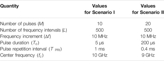
TABLE 1. LFM radar values of Scenario I (Abatzoglou and Gheen, 1998) and Scenario II (Zhang et al., 2017) were used for simulation.

TABLE 2

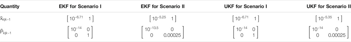
TABLE 2. Initial value of quantities used in simulations for Algorithm 1 and Algorithm 2.

For both Scenario I and Scenario II and for both estimators based on EKF and UKF, ${\mathbf{R}}_k={\sigma }_v^2\mathbf{I}$ (where ${\sigma }_v^2$ is obtained according to specified SNR). The SNR is defined as the relative strength of the signal with respect to noise; for this work, SNR = $\frac{h{\left({\mathbf{x}}_{k+1}\right)}^{T}h\left({\mathbf{x}}_{k+1}\right)}{n{\sigma }_v^2}$. The estimation of time delay and Doppler shift is obtained for 20 dB SNR; however, the comparative analysis is provided for various SNR ranging from $-30$ dB to 20 dB in decibels. In simulations, for UKF and for both Scenario I and Scenario II,$\kappa =0.5$ and 5 sigma points are considered according to $2n+1$ (where n is the dimension, which is 2 here). The estimators based on EKF and UKF in Algorithm 1 and Algorithm 2, respectively, are run for 5000 iterations, i.e., $K=5000$. The 100 Monte–Carlo (MC) trails are implemented to get statistically smooth NMSE and variance curves of EKF and UKF.

4.1 Estimation of Time Delay and Doppler Shift

The EKF- and UKF-based estimators were implemented with simulated data obtained using (Eq. 10, 11) over 5000 sampling intervals. The true data of states (obtained from Eq. 10) are used as reference values for comparison. The NMSE is given by

$NMS{E}_k\left(i\right)=\frac{1}{M_c}{\displaystyle \sum _{m_c=1}^{M_c}\frac{{\left({\mathbf{x}}_k^{m_c}\left(i\right)-{\widehat{\mathbf{x}}}_k^{m_c}\left(i\right)\right)}^2}{{\left({\mathbf{x}}_k^{m_c}\left(i\right)\right)}^2}},(18)$

where i is the index corresponding to time delay or Doppler shift. The NMSEs obtained from different estimators are shown in Figures 5, 6 for Scenario I and in Figures 7, 8 for Scenario II. The figures show a reduced NMSE as well as a faster convergence for the proposed EKF- and UKF-based estimators compared to the KLMS-Modified NC. Specifically, as shown in Figure 5, the EKF- and UKF-based estimators attain the final NMSE at around ${3000}^{th}$ iteration, and KLMS-Modified NC converges at around ${4500}^{th}$ iteration. Additionally, the final NMSE attained by EKF and UKF is significantly lower than the KLMS-Modified NC. Hence, though the estimators based on EKF, UKF, and KLMS-Modified NC take time to converge, the EKF- and UKF-based estimators converge fast and attain much lower final MSE as compared to the estimator based on KLMS-Modified NC. The reduced NMSE concludes an improved accuracy in estimation of time delay and Doppler shift with the proposed estimation techniques. The figures also conclude a relatively better accuracy for the UKF compared to the EKF. Also, as shown in Table 3, the relative computational complexity of EKF and UKF is similar and lower than KLMS-Modified NC and FFT as $n^3\ll ML$. However, in simulation, it is observed that the run time of UKF is 1.7 times higher as compared to the EKF. The 70 percent increase in run time accounts for the processing of $2n+1$ (for our case 5) sigma points. Therefore, because of the processing of multiple sigma points (which is not the case with the EKF), the run time of UKF is 1.7 times of EKF, where the 70 percent increase is because of the processing of 5 sigma points.

FIGURE 5

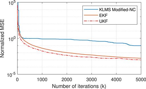
FIGURE 5. NMSE plots of time delay estimation using estimators based on KLMS-Modified NC, UKF, and EKF for Scenario I.

FIGURE 6

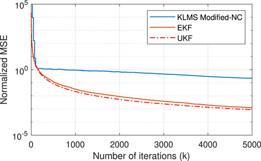
FIGURE 6. NMSE plots of Doppler shift estimation using estimators based on KLMS-Modified NC, UKF, and EKF for Scenario I.

FIGURE 7

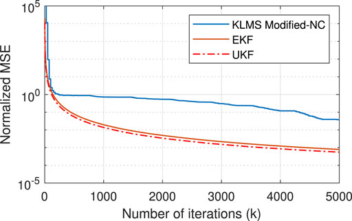
FIGURE 7. NMSE plots of time delay estimation using estimators based on KLMS-Modified NC, UKF, and EKF for Scenario II.

FIGURE 8

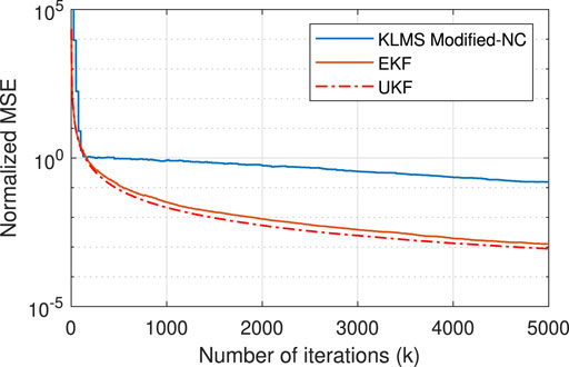
FIGURE 8. NMSE plots of Doppler shift estimation using estimators based on KLMS-Modified NC, UKF, and EKF for Scenario II.

TABLE 3

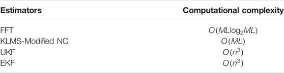
TABLE 3. Computational complexity of estimators based on FFT, KLMS-Modified NC, UKF, and EKF.

4.2 Performance Analysis With Varying SNR

The accuracy of the proposed estimation techniques for various SNRs is evaluated in terms of error variance. The error variance at the $k^{th}$ instant is given as

${\text{Ω}}_k^2\left(i\right)=\frac{1}{M_c}{\displaystyle \sum _{m_c=1}^{M_c}{\left({\mathbf{x}}_k^{m_c}\left(i\right)-{\widehat{\mathbf{x}}}_k^{m_c}\left(i\right)\right)}^2}.(19)$

The error variance in the estimation of time delay and Doppler shift is evaluated at various SNRs ranging from $-30$ dB to 20 dB. The variances are compared with the achievable analytical CRLBs for each of the time delay and Doppler shift. The CRLB analysis provides an efficient tool for performance analysis of the EKF- and UKF-based unbiased estimators (Cortina et al., 1991; Farina et al., 2002; Masarik and Subotic, 2016), as well as for their comparison with the existing estimators used for time delay and Doppler shift estimation. Masarik and Subotic (2016) derived the approximate expressions for the CRLB on the variance of unbiased estimates of the parameters of a narrow-band radar model in the presence of additive white Gaussian noise as well as interference with known structure. The derived CRLB expression is, however, suitable for the non-Bayesian estimation approach and cannot be applied to the Bayesian estimator as considered in this work. Therefore, in this work to derive the CRLB over the Bayesian estimate of ${\tau }_o$ and $f_d$, the following recursive expression of Fisher information matrix $\left({\mathbf{J}}_k\right)$ is used

${\mathbf{J}}_k\left(i,j\right)=-\mathbb{E}\left[\frac{{\partial }^2\left(\text{ln}\mathcal{P}\left({\mathbf{y}}_k,{\mathbf{x}}_k\right)\right)}{\partial {\mathbf{x}}_k\left(i\right)\partial {\mathbf{x}}_k\left(j\right)}\right];i,j=\mathrm{1,2}.(20)$

Here, ${\mathbf{x}}_k\left(i\right)$ is the $i^{th}$ element of ${\mathbf{x}}_k$, ${\mathbf{J}}_k\left(i,j\right)$ is the element at $i^{th}$ row and $j^{th}$ column of ${\mathbf{J}}_k$, and $\mathcal{P}(\cdot )$ is the joint probability density function.

From the work of Tichavsky et al. (1998), ${\text{J}}_{k+1}$ can be computed recursively as

${\mathrm{J}}_{k+1}={\mathrm{D}}_k^{22}-{\mathrm{D}}_k^{21}{\left({\mathrm{J}}_k+{\mathrm{D}}_k^{11}\right)}^{-1}{\mathrm{D}}_k^{12},(21)$

where

$\begin{array}{l}{\mathrm{D}}_k^{11}={\mathrm{F}}_k^T{\mathrm{Q}}_k^{-1}{\mathrm{F}}_k,\\ {\mathrm{D}}_k^{12}=-{\mathrm{F}}_k^T{\mathrm{Q}}_k^{-1}={\left[{\mathrm{D}}_k^{21}\right]}^T,\\ {\mathrm{D}}_k^{22}={\mathrm{Q}}_k^{-1}+{\mathrm{H}}^T{\mathrm{R}}_{k+1}^{-1}\mathrm{H}.\end{array}(22)$

The analytical expression of CRLB for time delay and Doppler shift is given by

$CRLB\left({\tau }_{ok}\right)={\mathrm{J}}_{k+1}^{-1}\left(\mathrm{1,1}\right),(23)$

$CRLB\left(f_{dk}\right)={\mathrm{J}}_{k+1}^{-1}\left(\mathrm{2,2}\right).(24)$

The variances obtained from the EKF, UKF, KLMS-Modified NC, and FFT are shown in Figures 9–12. As shown in the figures, the variances obtained with the EKF and UKF are closer to the achievable CRLB in comparison to the KLMS-Modified NC and FFT. Moreover, the figures validate a marginally better accuracy for the UKF compared to the EKF.

FIGURE 9

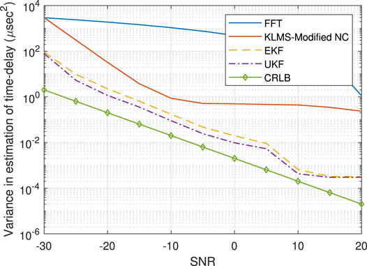
FIGURE 9. Variance in the estimation of time delay using estimation techniques based on UKF, EKF, KLMS-Modified NC, and FFT for Scenario I.

FIGURE 10

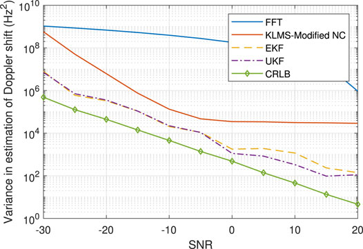
FIGURE 10. Variance in the estimation of Doppler shift using estimation techniques based on UKF, EKF, KLMS-Modified NC, and FFT for Scenario I.

FIGURE 11

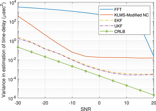
FIGURE 11. Variance in the estimation of time delay using estimation techniques based on UKF, EKF, KLMS-Modified NC, and FFT for Scenario II.

FIGURE 12

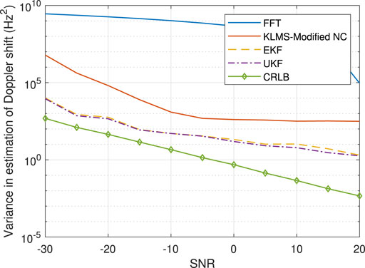
FIGURE 12. Variance in the estimation of Doppler shift using estimation techniques based on UKF, EKF, KLMS-Modified NC, and FFT for Scenario II.

5 Conclusion

Increasing applications of target tracking in space technology, defense systems, and ocean exploration requires radar systems with a highly accurate estimator. The target tracking is based on the estimation of the target’s unknown parameters (time delay and Doppler shift) from the returning signal. The recently introduced nonlinear estimator based on KLMS-Modified NC can significantly improve the accuracy compared to conventional linear estimators. However, its practical utility is limited by the longer convergence time and parameter modeling errors. Hence, to circumvent these shortcomings, in this paper, two new nonlinear estimation techniques, based on EKF and UKF, are proposed. Significantly, EKF estimates the target’s unknown parameters by linearly approximating the system nonlinearity. This significant approximation may lead EKF to suffer from poor estimation accuracy (particularly in complex environments). The UKF, unlike EKF, instead of linearly approximating the system nonlinearity, considers the true nonlinear model for estimation. Consequently, UKF shows better stability in comparison to EKF and is found to yield estimates with slightly better/similar accuracy. Further, to access the comparative performance of the proposed estimation techniques with the existing nonlinear estimator and linear estimator, CRLBs are used as a benchmark. Lastly, simulations performed over realistic LFM radar systems reveal that the proposed nonlinear estimation techniques based on EKF and UKF outperform the recently introduced nonlinear estimator based on KLMS-Modified NC and linear estimation technique based on FFT. Also, the variance yields in the estimation of the time delay and Doppler shift by the proposed estimators are found closer to the corresponding CRLBs.

In the proposed work, the nonlinear version of the Kalman filter (EKF and UKF) suitable for Gaussian perturbation is explored. However, in practice, the presence of clutter, usually model by non-Gaussianity, is ubiquitous. Therefore, in future, to handle the effects of clutter, the nonlinear version of the Kalman filter capable of dealing with non-Gaussianity can be explored. Also, for accurate tracking, the tracker requires range, radial velocity, and angle information. In light of this, the possible challenge of the proposed approach would be how to estimate the angle information at the signal level itself. We left the estimation of angle using the proposed technique as a future work.

Data Availability Statement

The original contributions presented in the study are included in the article/Supplementary Material; further inquiries can be directed to the corresponding author.

Author Contributions

US: writing and simulations. AS: writing, provided feedback for simulations and provided reviews on the manuscript. VB: proposing the main Idea and provided reviews on the manuscript. AM: providing reviews on the manuscript.

Funding

This work is an outcome of the research and development work undertaken project under the Visvesvaraya PhD Scheme of the Ministry of Electronics and Information Technology, Government of India, being implemented by Digital India Corporation. The research of Abhinoy Kumar Singh is funded by the Department of Science and Technology, Government of India, under the scheme of Inspire Faculty Award. While pursuing a Postdoc at the Interdisciplinary Centre for Security, Reliability and Trust (SnT), University of Luxembourg, the work has been submitted as a part of a PhD work.

Conflict of Interest

The authors declare that the research was conducted in the absence of any commercial or financial relationships that could be construed as a potential conflict of interest.

Publisher’s Note

All claims expressed in this article are solely those of the authors and do not necessarily represent those of their affiliated organizations, or those of the publisher, the editors and the reviewers. Any product that may be evaluated in this article, or claim that may be made by its manufacturer, is not guaranteed or endorsed by the publisher.

Footnotes

¹In this work, the target is assumed to be a perfect reflector; hence, the effect of amplitude attenuation is not considered in the scattered signal.

²The subscript i in fi(t) denotes that f(t) is the instantaneous frequency. Here, i is only used for nominating fi(t) as an instantaneous frequency.

References

Abatzoglou, T. J., and Gheen, G. O. (1998). Range, Radial Velocity, and Acceleration MLE Using Radar LFM Pulse Train. IEEE Trans. Aerosp. Electron. Syst. 34, 1070–1083. doi:10.1109/7.722676

CrossRef Full Text | Google Scholar

Anderson, B. D., and Moore, J. B. (2012). Optimal Filtering (Courier Corporation). New York: Dover Publications.

Arasaratnam, I., and Haykin, S. (2009). Cubature Kalman Filters. IEEE Trans. Automat. Contr. 54, 1254–1269. doi:10.1109/tac.2009.2019800

CrossRef Full Text | Google Scholar

Arulampalam, M. S., Maskell, S., Gordon, N., and Clapp, T. (2002). A Tutorial on Particle Filters for Online Nonlinear/non-Gaussian Bayesian Tracking. IEEE Trans. Signal. Process. 50, 174–188. doi:10.1109/78.978374

CrossRef Full Text | Google Scholar

Athans, M., Wishner, R., and Bertolini, A. (1968). Suboptimal State Estimation for Continuous-Time Nonlinear Systems from Discrete Noisy Measurements. IEEE Trans. Automat. Contr. 13, 504–514. doi:10.1109/tac.1968.1098986

CrossRef Full Text | Google Scholar

Bar-Shalom, Y., Li, X. R., and Kirubarajan, T. (2004). Estimation with Applications to Tracking and Navigation: Theory Algorithms and Software. John Wiley & Sons.

Brown, R. G., and Hwang, P. Y. (1992). Introduction to Random Signals and Applied Kalman Filtering, Vol.3. New York: Wiley.

Buzzi, S., Lops, M., Venturino, L., and Ferri, M. (2008). Track-before-detect Procedures in a Multi-Target Environment. IEEE Trans. Aerosp. Electron. Syst. 44, 1135–1150. doi:10.1109/taes.2008.4655369

CrossRef Full Text | Google Scholar

Chang, L., Hu, B., Li, A., and Qin, F. (2013). Transformed Unscented Kalman Filter. IEEE Trans. Automat. Contr. 58, 252–257. doi:10.1109/tac.2012.2204830

CrossRef Full Text | Google Scholar

Cortina, E., Otero, D., and D'Attellis, C. E. (1991). Maneuvering Target Tracking Using Extended Kalman Filter. IEEE Trans. Aerosp. Electron. Syst. 27, 155–158. doi:10.1109/7.68158

CrossRef Full Text | Google Scholar

Farina, A., Ristic, B., and Benvenuti, D. (2002). Tracking a Ballistic Target: Comparison of Several Nonlinear Filters. IEEE Trans. Aerosp. Electron. Syst. 38, 854–867. doi:10.1109/taes.2002.1039404

CrossRef Full Text | Google Scholar

Gu, T., Liao, G., Li, Y., Quan, Y., Guo, Y., and Huang, Y. (2019). An Impoved Parameter Estimation of Lfm Signal Based on MCKF. IEEE Int. Geosci. Remote Sensing Sympo, 596–599. doi:10.1109/igarss.2019.8898485

CrossRef Full Text | Google Scholar

Jian Li, J., and Renbiao Wu, R. (1998). An Efficient Algorithm for Time Delay Estimation. IEEE Trans. Signal. Process. 46, 2231–2235. doi:10.1109/78.705444

CrossRef Full Text | Google Scholar

Jiang, Z., Song, Q., He, Y., and Han, J. (2007). “A Novel Adaptive Unscented Kalman Filter for Nonlinear Estimation.”in 46th Conf. Decision Control IEEE, New Orleans, LA, December 12–14, 2007, 4293–4298. doi:10.1109/cdc.2007.4434954

CrossRef Full Text | Google Scholar

Julier, S. J., and Uhlmann, J. K. (1997). New Extension of the Kalman Filter to Nonlinear systemsSignal Processing, Sensor Fusion, and Target Recognition VI. Int. Soc. Opt. Photon.) 3068, 182–194. doi:10.1117/12.280797

CrossRef Full Text | Google Scholar

Julier, S. J., and Uhlmann, J. K. (2004). Unscented Filtering and Nonlinear Estimation. Proc. IEEE 92, 401–422. doi:10.1109/jproc.2003.823141

CrossRef Full Text | Google Scholar

Julier, S., Uhlmann, J., and Durrant-Whyte, H. F. (2000). A New Method for the Nonlinear Transformation of Means and Covariances in Filters and Estimators. IEEE Trans. Automat. Contr. 45, 477–482. doi:10.1109/9.847726

CrossRef Full Text | Google Scholar

Kay, S. M. (1993). Fundamentals of Statistical Signal Processing: Estimation Theory. Upper Saddle River, NJ: Prentice Hall PTR.

Koteswara Rao, S. (2005). Modified Gain Extended Kalman Filter with Application to Bearings-Only Passive Manoeuvring Target Tracking. IEE Proc. Radar Sonar Navig. 152, 239–244. doi:10.1049/ip-rsn:20045074

CrossRef Full Text | Google Scholar

Kulikov, G. Y., and Kulikova, M. V. (2015). The Accurate Continuous-Discrete Extended Kalman Filter for Radar Tracking. IEEE Trans. Signal. Process. 64 (4), 948–958. doi:10.1109/TSP.2015.2493985

Google Scholar

Kwon, J., Kwak, N., Yang, E., and Kim, K. (2019). “Particle Filter Based Track-Before-Detect Method in the Range-Doppler Domain, in ” 2019 IEEE Radar Conference (RadarConf) (IEEE), Boston, Massachusetts, April 22–26, 2019, 1–5. doi:10.1109/radar.2019.8835620

CrossRef Full Text | Google Scholar

Levanon, N., and Mozeson, E. (2004). Radar Signals. John Wiley & Sons.

Liu, W., Pokharel, P. P., and Principe, J. C., (2008). The Kernel Least-Mean-Square Algorithm. IEEE Trans. Signal. Process. 56, 543–554. doi:10.1109/tsp.2007.907881

CrossRef Full Text | Google Scholar

Liu, W., Principe, J. C., and Haykin, S. (2011). Kernel Adaptive Filtering: A Comprehensive Introduction, vol.57. John Wiley & Sons.

Masarik, M. P., and Subotic, N. S. (2016). “Cramer-Rao Lower Bounds for Radar Parameter Estimation in Noise Plus Structured Interference.” in IEEE Radar Conference, Philadelphia, PA, May 2–6, 2016 1–4. IEEE.

PubMed Abstract | Google Scholar

Mitra, R., and Bhatia, V. (2017). Finite Dictionary Techniques for MSER Equalization in RKHS. SIViP 11, 849–856. doi:10.1007/s11760-016-1031-1

CrossRef Full Text | Google Scholar

Mitra, R., and Bhatia, V. (2014). The Diffusion-KLMS Algorithm. in Int. Conf. Inf. Technology (IEEE), Bhubaneswar, Odisha, India, December 22–24, 2014, 256–259. doi:10.1109/icit.2014.33

CrossRef Full Text | Google Scholar

Richards, M. A. (2005). Fundamentals of Radar Signal Processing. New York: Tata McGraw-Hill Education.

Richards, M. A., Scheer, J., Holm, W. A., and Melvin, W. L. (2010). Principles Of Modern Radar (Citeseer). New Jersey: SciTech Publishing.

Rife, D., and Boorstyn, R. (1974). Single Tone Parameter Estimation from Discrete-Time Observations. IEEE Trans. Inform. Theor. 20, 591–598. doi:10.1109/tit.1974.1055282

CrossRef Full Text | Google Scholar

Singh, A. K., Radhakrishnan, R., Bhaumik, S., and Date, P. (2018). Adaptive Sparse-Grid Gauss-Hermite Filter. J. Comput. Appl. Math. 342, 305–316. doi:10.1016/j.cam.2018.04.006

CrossRef Full Text | Google Scholar

Singh, U. K., Mitra, R., Bhatia, V., and Mishra, A. K. (2019). Kernel LMS-Based Estimation Techniques for Radar Systems. IEEE Trans. Aerosp. Electron. Syst. 55, 2501–2515. doi:10.1109/taes.2019.2891148

CrossRef Full Text | Google Scholar

Singh, U. K., Mitra, R., Bhatia, V., and Mishra, A. K. (2017). Target Range Estimation in OFDM Radar System via Kernel Least Mean Square Technique. Int. Conf. Radar Syst., 1–5. doi:10.1049/cp.2017.0409

CrossRef Full Text | Google Scholar

Taek Song, T., and Speyer, J. (1985). A Stochastic Analysis of a Modified Gain Extended Kalman Filter with Applications to Estimation with Bearings Only Measurements. IEEE Trans. Automat. Contr. 30, 940–949. doi:10.1109/tac.1985.1103821

CrossRef Full Text | Google Scholar

Tichavsky, P., Muravchik, C. H., and Nehorai, A. (1998). Posterior Cramer-Rao Bounds for Discrete-Time Nonlinear Filtering. IEEE Trans. Signal. Process. 46, 1386–1396. doi:10.1109/78.668800

CrossRef Full Text | Google Scholar

Yang, L., Su, W., and Hong, G. (2011). Velocity estimation of moving target using generalized-MUSIC based on stepped-frequency-pulse-train signal. Int. Conf. Radar. vol. 1, 331–334. doi:10.1109/CIE-Radar.2011.6159544

CrossRef Full Text | Google Scholar

Zhan, R., and Wan, J. (2007). Iterated Unscented Kalman Filter for Passive Target Tracking. IEEE Aerosp. Electron. Syst. Mag. 43, 1155–1163. doi:10.1109/taes.2007.4383605

CrossRef Full Text | Google Scholar

Zhang, Y.-X., Hong, R.-J., Pan, P.-P., Deng, Z.-M., and Liu, Q.-F. (2017). Frequency Domain Range Sidelobe Correction in Stretch Processing for Wideband LFM Radars. IEEE Trans. Aerosp. Electron. Syst. 53, 111–121. doi:10.1109/taes.2017.2649278

CrossRef Full Text | Google Scholar