 Miloš Prágr
 Jan Bayer
 Jan Faigl
- Computational Robotics Laboratory, Faculty of Electrical Engineering, Czech Technical University in Prague, Prague, Czechia
In this study, we address generalized autonomous mobile robot exploration of unknown environments where a robotic agent learns a traversability model and builds a spatial model of the environment. The agent can benefit from the model learned online in distinguishing what terrains are easy to traverse and which should be avoided. The proposed solution enables the learning of multiple traversability models, each associated with a particular locomotion gait, a walking pattern of a multi-legged walking robot. We propose to address the simultaneous learning of the environment and traversability models by a decoupled approach. Thus, navigation waypoints are generated using the current spatial and traversability models to gain the information necessary to improve the particular model during the robot’s motion in the environment. From the set of possible waypoints, the decision on where to navigate next is made based on the solution of the generalized traveling salesman problem that allows taking into account a planning horizon longer than a single myopic decision. The proposed approach has been verified in simulated scenarios and experimental deployments with a real hexapod walking robot with two locomotion gaits, suitable for different terrains. Based on the achieved results, the proposed method exploits the online learned traversability models and further supports the selection of the most appropriate locomotion gait for the particular terrain types.
1 Introduction
The presented online terrain learning approach is motivated by long-term missions where autonomous robots would improve their operational performance in navigating a priori unknown environments. Some difficult to traverse terrains, such as large rocks, can be identified as obstacles using an observed geometric model of the environment. However, areas which appear flat and thus easy to traverse may, in practice, be hard to traverse due to their terra-mechanical properties, as experienced by NASA’s Mars Rover Spirit stuck in soft sand (Brown and Webster, 2010). In the presented approach, individual terra-mechanical properties are assumed to be partially unknown, and we learn a black box model to assess the traversability in a particular environment from the terrain appearance (Prágr et al., 2018). Since the scope of the functional relation between the terrain appearance and traversability might be limited to a particular environment, we advocate that on long-term deployments and exploration missions, the terrain models are learned online incrementally (Prágr et al., 2019b) as a part of the mission (Prágr et al., 2019a). Hence, we focus on the exploration of the environment and its terra-mechanical properties represented as the traversal costs that characterize the difficulty of traversing the individual terrains, as visualized in Figure 1. In particular, we consider multi-legged walking robots that can traverse various terrains with different traversal costs (also depending on the particular locomotion gait used), which provide a representative case for demonstrating the benefits of traversability assessment learned online. Compared to the previous work, the presented approach addresses the different locomotion gaits of the robot and distinguishes individual terrain-gait traversal cost models. In addition, the proposed exploration strategy provides a non-myopic (Zlot and Stentz, 2006) solution that takes into account both the spatial exploration and learning of the traversal cost models.
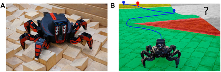
FIGURE 1. (A) Hexapod walking robot (courtesy of Forouhar et al. (2021)) (B) and its deployment using the proposed approach. The visualized planned path is to visit determined exploration goals for the spatial (in blue) and traversal cost models (in red). The spatial exploration goals are located close to the boundary of the already explored part of the environment. The traversal cost exploration goals correspond to sites where the terrain traversal cost model can be improved. Since the cost model is already partially learned, the red-tinted turf is known to be hard to traverse, and thus the robot prefers the green-tinted pavement, which is relatively easy to traverse. The yellow-tinted terrain is yet to be experienced by the robot and thus carries the terrain learning goal indicated by the red waypoint. The not-yet-observed area is gray.
In the proposed approach, the impassable parts of the explored environment are determined by the geometric models using a grid-based elevation map (Bayer and Faigl, 2019). The individual terrain-gait traversal cost models are near-to-far predictors that infer the time to traverse over the traversable areas from their appearance and are learned using the robot’s previous experience accrued when traversing similar-appearing terrains using a particular gait. The traversal cost models comprise Gaussian process (GP) regressors (Rasmussen and Williams, 2006), which predict the traversal costs from the terrain appearance, and growing neural gas (GNG) (Fritzke, 1994) terrain type clustering schemes used to identify similar-appearing terrains. The geometric and traversal cost models are incrementally constructed while exploring the mission environment. The geometric model is continually built from the robot’s exteroception, whereas each traversal cost model accumulates the costs experienced by the robot when moving using the respective locomotion gait. During the deployment, each model continually provides a set of exploration goals to be visited to learn (improve) the model. For several possible goal locations, the exploration strategy is to determine a sequence of the navigational goals to be visited that is addressed as a solution of the Generalized Traveling Salesman Problem (GTSP) (Noon, 1988) to provide a non-myopic solution considering the so-called TSP distance cost (Faigl and Kulich, 2013).
The remainder of the article is organized as follows. In Section 2, we present an overview of the related approaches in mobile robot exploration and traversability assessment. Section 3 formally defines the studied problem of mobile robot exploration with a priori unknown terrain traversal cost assessment. The proposed exploration with online traversal cost learning is presented in Section 4. Section 5 reports on the performed experimental results in simulations and real-world experimental deployments with a multi-legged robot controlled by two motion gaits. In Section 6, we discuss the strong points and limitations of the proposed approach. Section 7 concludes the study.
2 State of the art
This section presents an overview of works related to the proposed approach. First, we focus on the traversability assessment approaches. Then we survey mobile robot exploration and environment modeling.
2.1 Mobile robot traversability
Two main questions emerge when reasoning about robot traversability over terrains. First, can the terrain be safely traversed, or should it be avoided? Second, if the terrain is passable, how does it compare to other terrains, i.e., is it easier and safer to traverse? Note that for the sake of clarity, we further denote the binary (true/false) traversability, which determines whether an area is an impassable obstacle or passable terrain, as terrain passability. In contrast, the relative comparison of the traversal difficulty over passable terrains is denoted as assessing the traversal cost. The term traversability is used to describe the notion in general, including both the passability and traversal cost. A review of mobile robot traversability assessment methods can be found in Papadakis (2013), and an overview of learning-based methods for ground robot navigation is in Guastella and Muscato (2021). Hence, we focus on works relevant to how traversability is approached in this study.
The passability discrimination can be directly incorporated in mapping in the form of occupancy cell grids (Moravec and Elfes, 1985), Gaussian mixtures (O’Meadhra et al., 2019), GP models (O’Callaghan et al., 2009), or Hilbert maps (Ramos and Ott, 2016). The distinction of terrain passability can be understood as an instance of terrain classification, where terrains are assigned individual classes, and each class carries presumed terra-mechanical properties. For example, some classes can be considered hard-to-traverse vegetation or obstacles (Bradley et al., 2015). In addition to terrain classification, terrains can be assigned continuous values describing some observed terrain property such as roughness (Krüsi et al., 2016; Belter et al., 2019), slope (Stelzer et al., 2012), or step height (Homberger et al., 2016; Wermelinger et al., 2016). For continuous measures, passability can be based on thresholding the value, as in Stelzer et al. (2012), where the passability is determined by individually thresholding terrain slope, roughness, and step height. Moreover, classes may correspond to a particular robot configuration, such as in Haddeler et al. (2020), where the authors classify terrains into modes of wheeled-legged locomotion.
In instances where the terra-mechanical properties are unknown and thus terrains’ appearance and geometry features are not sufficient to determine their traversability, the traversability can be based on the robot’s prior experience with similar terrains. The experience-based measures can be derived from the robot proprioception and described using stability (McGhee and Frank, 1968; Lin and Song, 1993), slippage (Gonzalez and Iagnemma, 2018), vibrations (Bekhti and Kobayashi, 2016), velocity, or energy consumption (Kottege et al., 2015). The experience-based approaches describe the traversal cost only over passable terrains since the traversal is needed to acquire the robot experience. An exception worth mentioning is haptic sensing to determine obstacle passability (Baleia et al., 2015), which, however, still relies on the direct interaction of the robot with the terrain.
Since the experience-based approaches use on-location robot experience, they are difficult to use directly in path planning where it is necessary to evaluate terrain traversability from a distance using only exteroceptive measurements. Near-to-far approaches pair traversability indicators that can be observed only near the robot (such as proprioception or dense short-range measurements) with terrain appearance and geometry that can be observed from farther distances and thus learn to predict traversability from the long-range measurements. Sofman et al. (2006) incrementally learned the relation between dense laser-based features characterizing ground unit traversability and overhead features that can be used to assess traversability from aerial images, whereas Bekhti and Kobayashi (2016) learned to predict vibration-based traversability from terrain texture. Quann et al. (2020) proposed an energy traversal cost regressor considering both terrain position and appearance. In addition, Mayuku et al. (2021) proposed a self-supervised labeling approach for a near-to-far scenario, where vibration-based traversal cost is inferred from image data, and the self-supervised data gathering is based on identified terrain classes.
Following the approaches in the literature, we assume that terrain is rigid, and it is possible to distinguish passable terrain and non-traversable obstacles from the terrain geometry using a step height similar to Stelzer et al. (2012), or Wermelinger et al. (2016). Hence, this study focuses on modeling the traversal cost over the determined passable terrains. Moreover, we are motivated by the online cost assessment in mobile robot exploration, where the computational requirements are crucial. Therefore, we avoid high fidelity models, which besides being costly to compute also rely on plan execution with high precision (such as deterministic foothold placement), which might not be available in practice. The traversal cost is thus learned as a black box near-to-far model that uses terrain appearance to predict the time to traverse over terrains. Since the scope of the relation between the terrain appearance and traversability might be limited to a particular environment, we incrementally learn the cost predictor by sampling the robot’s experience with traversing individual terrains. Similar to the classification in Belter et al. (2019), a color histogram is selected as the terrain appearance descriptor because it is simple to compute and the histograms are sufficiently descriptive to capture multi-colored terrains. Furthermore, we consider locomotion gaits of the employed hexapod walking robot that are suitable for different terrains. Thus, the passable terrain is a terrain traversable by at least one gait, and obstacles are terrain parts that none of the gaits can traverse. We propose a decoupled approach that predicts the traversal cost for each gait independently, and the robot then selects the most cost-efficient gait for each terrain.
Regarding the existing methods, the proposed approach is closest to Haddeler et al. (2020), where modes of the wheeled-legged robot are switched. In addition, the proposed approach is also close to the self-supervised, near-to-far traversability-learning approach proposed by Mayuku et al. (2021). In that regard, the primary contribution of the proposed approach is the integration of active traversability learning in mobile robot exploration, where the robot plans a non-myopic path to improve both the spatial and traversal cost models learned online during the deployment.
2.2 Mobile robot exploration and environment modeling
Mobile robot exploration is an active perception problem that concerns behaviors where the robot seeks to build a model of a priori unknown environment. The exploration entails the robot seeking areas that are in some capacity unknown to construct a map of the environment. The exploration thus inherently combines localization, navigation, and planning (Schultz et al., 1999) to decide where the robot should go next. Steering the robot navigation to not-yet-observed areas yields frontier-based exploration (Yamauchi, 1997), where the frontiers represent boundaries between the observed traversable area and the unknown space represented on an occupancy grid (Moravec and Elfes, 1985). Recently, in the octree-based environment model, frontiers are represented as mesh faces with few neighbors (Azpúrna et al., 2021).
Bourgault et al. (2002) and Makarenko et al. (2002) exploit the probabilistic representation on such an occupancy evidence grid and navigate to maximize the approximated occupancy information gain. Charrow et al. (2015) proposed to use Cauchy–Schwarz quadratic mutual information to speed up the information gain computation. In addition, approaches that rely on non-grid-based representation for navigation, such as meshes and topological maps, may retain cell or voxel grids to quantify the information gain (Dang et al., 2020).
In addition to mapping, robots also build models of environment-underlying phenomena that can be temperature models (Luo and Sycara, 2018) or spread of gas (Rhodes et al., 2020). The environment phenomenon can be considered spatial, and the goal is thus to learn the mapping from the position in the environment to the value of the phenomenon. Furthermore, a spatiotemporal model can be considered (Ma et al., 2018) that would require repeatedly visiting particular areas to build the temporal model, which might be needed for changing environments (Krajník et al., 2017).
Spatial-based modeling can be considered as informative path planning (Singh et al., 2007), where the goal is to find the most informative path through the environment (Hollinger and Sukhatme, 2014) subject to a particular constraint such as the robot energy budget (Binney and Sukhatme, 2012). Informative path planning approaches can be broadly divided into myopic and non-myopic methods. The myopic methods are greedy and plan only with regard to the next goal, whereas non-myopic methods plan with a longer horizon. For example, in the context of frontier-based mobile robot exploration, seeking the closest frontier is myopic, contrary to path planning to visit all the representatives of the frontiers that is non-myopic (Faigl et al., 2012).
Like seeking frontiers in spatial exploration, the explorer learning an underlying model must actively locate sites to sample novel information. Hence, GP regressors (Rasmussen and Williams, 2006) are particularly suited for active learning because it is relatively straightforward to identify uncertain regions where the model should be improved. GP prediction uncertainty is characterized by the differential entropy of the predicted normal distribution, leading to the characterization of information gained by observing individual areas. However, in practice, directly computing the information gained by possible observations is not feasible due to the number of possible actions, especially for a long planning horizon. Hence, various approximations and sampling strategies have been proposed.
Pasolli and Melgani (2011) proposed to either directly seek the most uncertain samples signified by the highest prediction variance or to select areas that are the most remote in the feature space given the GP hyper-parameters. In Viseras et al. (2019), the robot selects paths with high average entropy per sampling to tradeoff informativeness and the number of samplings. Martin and Corke (2014) proposed to set the mean function of a GP traversal cost regressors to zero, thus motivating a robot to traverse unknown areas where the predictions are close to the zero mean. The GP Upper Confidence Bound (GP-UCB) (Srinivas et al., 2010) is an exploration–exploitation method that combines seeking the most uncertain areas with improving the model around the highest value. It can be used when the learner is interested in finding extreme values of the modeled phenomenon, such as temperature (Luo and Sycara, 2018; Shi et al., 2020). In addition, a depth-first variant of the Monte Carlo Tree Search (MCTS) to select anytime informative paths can be employed to consider both differential entropy and upper confidence bound to model sampling informativeness (Guerrero et al., 2021).
Karolj et al. (2020) computed a path to the closest spatial frontier that visits all local sampling locations for a magnetism model by solving the Traveling Salesman Problem (TSP) over the respective goal locations. In localization in mapping, Ossenkopf et al. (2019) note that occupancy information gained at an unknown location holds little value and thus weight the occupancy gains by a pose uncertainty (Vallvé and Andrade-Cetto, 2015). Hence, the explorer must address how to combine the occupancy and pose uncertainties. In Bourgault et al. (2002) and Stachniss et al. (2005), the total exploration utility is a linear combination of the occupancy uncertainty and the robot localization uncertainty represented using the differential entropy based on its position distribution. In Carrillo et al. (2018), it is argued that combining Shannon’s discrete and differential entropies is neither practical nor sound because the differential entropy is neither invariant under a change of variable nor dimensionally correct. Therefore, both quantities may differ significantly in value. Consequently, Carrillo et al. (2018) proposed to use the localization uncertainty to weigh the Rényi entropy (Rényi, 1961) of the occupancy grid.
Based on the literature review on exploration approaches, we propose to generalize the previous work (Prágr et al., 2019a) toward a non-myopic approach. The therein proposed method combines active learning of traversal cost over terrains with spatial exploration using a greedy approach. The approximated spatial information gains and cost models are derived from Shannon’s discrete and differential entropies, respectively. Considering the reasoning of Carrillo et al. (2018), we avoid a direct combination of these two values in this study. In addition, we aim to build a modular system that supports the learning of models that range from the spatial map and cost predictors used in this study to temperature and pollution models. Hence, instead of creating a combined information gain utility function using the Rényi entropy, which is suitable for the combination of a map and robot’s localization model used by Carrillo et al. (2018), we elect to use a policy that combines the spatial exploration and cost learning goals (and goals reported by any additional model), similarly to the approach proposed by Karolj et al. (2020).
However, unlike the therein-built magnetism model, a spatial GP, we assume that the terrain traversal cost correlates with the terrain appearance. Therefore, the GP regressor infers the cost from the terrain feature descriptors instead of the terrain location. Consequently, rather than terrains nearby, sampling the cost to traverse an unknown terrain primarily affects the predictions over similarly appearing terrains close in the feature space. The affected terrains are determined using a terrain clustering scheme. Incremental growing neural gas (IGNG) (Prudent and Ennaji, 2005) is used to continually construct the terrain class structure, in which each class is assigned traversal cost and sampling reward (information gain) based on the GP’s predictions. As a result, we model the computation of the goal visit sequence as an instance of the Generalized TSP (GTSP) (Noon, 1988) (also called the Set TSP), which is a variant of the TSP where nodes are grouped into mutually exclusive and exhaustive sets. The problem is then to visit each set instead of visiting each node. In the context of the proposed exploration approach, the individual nodes correspond to possible sampling locations, and the sets are either terrain classes extracted from the cost prediction model or places where the robot can observe areas unknown to the spatial model.
The problem of mobile robot exploration with traversal cost learning is defined in the next section, whereas the strengths and weak points of the proposed approach are further discussed in Section 6.
3 Problem specification
The addressed exploration using an autonomous hexapod walking robot combines spatial exploration with active learning of terrain traversal cost models. The environment is modeled as a 2D grid
where n is the number of cells in the respective sequence, the function 8 nb(ν) lists the cells in the 8-neighborhood of ν, and π(ν) = 1 indicates that the cell ν is passable. In addition, the robot can use a discrete set of walking gaits
FIGURE 2. Footprint around the robot position covers the cells with potential multi-legged walking robot footholds.
The robot desires to move through the environment as efficiently as possible with respect to (w.r.t.) the cost C. Therefore, it moves along the cheapest path between ν and ν′.
where Ψ(ν, ν′) is the space of all paths from ν to ν′. The cost C(ψ) of traversing ψ represents a generic path cost such as time to traverse or expected consumed energy; without the loss of generality, the time to traverse is the cost of choice in this study. It is assumed that the cost is additive, thus permitting to combine the costs of two consecutive path segments ψa and ψb into the cost of the combined path ψa ⊕ ψb as follows:
where ⊕ denotes the concatenation of the paths. The cost of a path is decomposed to the sequence of costs to traverse from passable cell νa to its neighbor νb.
where ‖(νa, νb)‖ is the Euclidean distance between the cells (i.e., either dν or
In the spatial exploration, the robot builds the geometry model
3.1 Traversal cost modeling
The traversal cost is assumed to be too complex to be assessed only from the terrain geometry. In this study, the task is to learn a traversal cost predictor
The learned model is compared to the uninformed baseline that represents a robot that only explores the spatial map and does not learn the cost models and thus uses the optimistic flat cost model.
where vmax is the maximum robot velocity over all
The proposed approach is evaluated in model scenarios as follows. First, the robot is set to explore the environment
4 Proposed system for active terrain learning in exploration
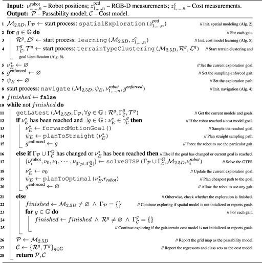
In this section, we describe the proposed system for active terrain learning and exploration, which is overviewed in Figure 3. During the exploration, which yields the spatial geometric passability model
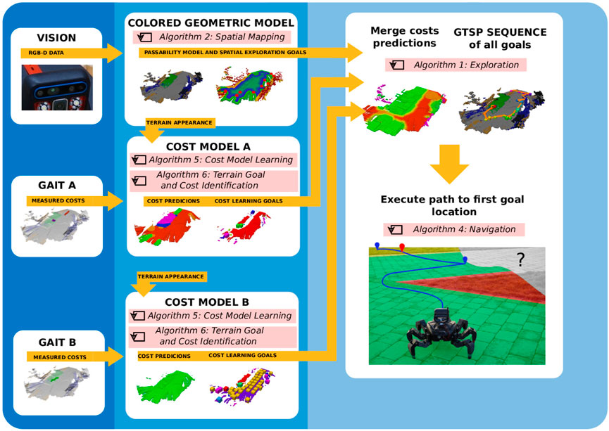
FIGURE 3. An overview of the proposed exploration system. The robot uses the RGB-D data to build the color elevation model of the environment in which it identifies the passable areas (Algorithm 2). The terrain appearance stored in the model is paired with the costs experienced by the robot to learn the traversal cost models for the individual locomotion gaits (Algorithm 5 and Algorithm 6). The cost predictions for the individual gaits and the terrain passability are used to plan the exploration path in a TSP sequence (Algorithm 1) over every goal reported by the geometric and cost models. The robot navigates to the first goal in the sequence (Algorithm 4).
In the rest of the section, we describe the exploration process. The symbols used in the description are listed in Table 1. First, we show how the GTSP is used to find the exploration path. Then we show the geometric environment model in detail and the related passability model
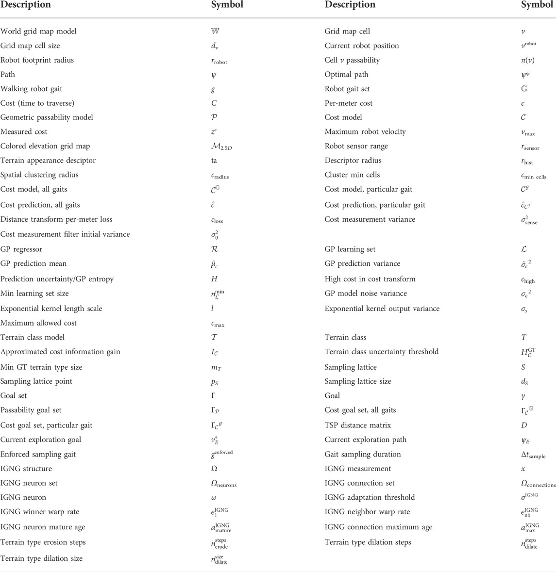
TABLE 1. Used symbols.
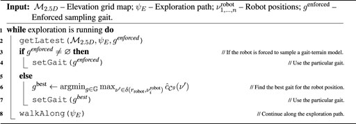
4.1 Exploration
The robot explores the passability model
Given the current robot position
A total of two transforms are applied to the distance matrix D to create an open instance of the GTSP. First, the robot does not need to return to its current position after exploring the environment. Hence, the problem is transformed by setting the cost to reach the current robot position from any goal as zero
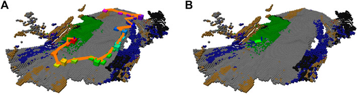
FIGURE 4. An example of a planned exploration path. (A) Global path over the sequence of goals determined by the TSP solver; (B) the local path to the first goal.
The plan is recomputed on-demand either when there is a change in the goal set or as a result of reaching the current goal. Moreover, upon reaching a cost model goal, the robot switches to the model’s respective gait genforced and is forced to move forward for Δtsample (or until an obstacle is reached) to sample the traversal cost over the terrain. The exploration ends when every model reports zero goals. The exploration process is summarized in Algorithm 1.
Algorithm 1. Exploration.
4.2 Environment geometry & passability model
The grid environment
Algorithm 2. Spatial exploration.

We define the passability of the cell
where 8 nb(ν) is the 8-neighborhood of the cell ν, and the step height Δ(νa, νb) is as follows:
where elevation(ν) denotes the estimated height of the terrain at ν. The probability that the robot can pass a cell ν is as follows:
where the threshold ρobstacle represents the lowest obstacle to be detected. An example of the grid map is shown in Figure 5A.In active perception scenarios, the information about the terrain model
where k(ν) is the number of the unknown cells in the neighborhood of ν. Thus, the expected information gained by perceiving the terrain from the position of the cell ν can be expressed as follows:
where δ(rsensor, ν) is the sensor range rsensor-large neighborhood of ν; the function observable (ν, ν′) returns
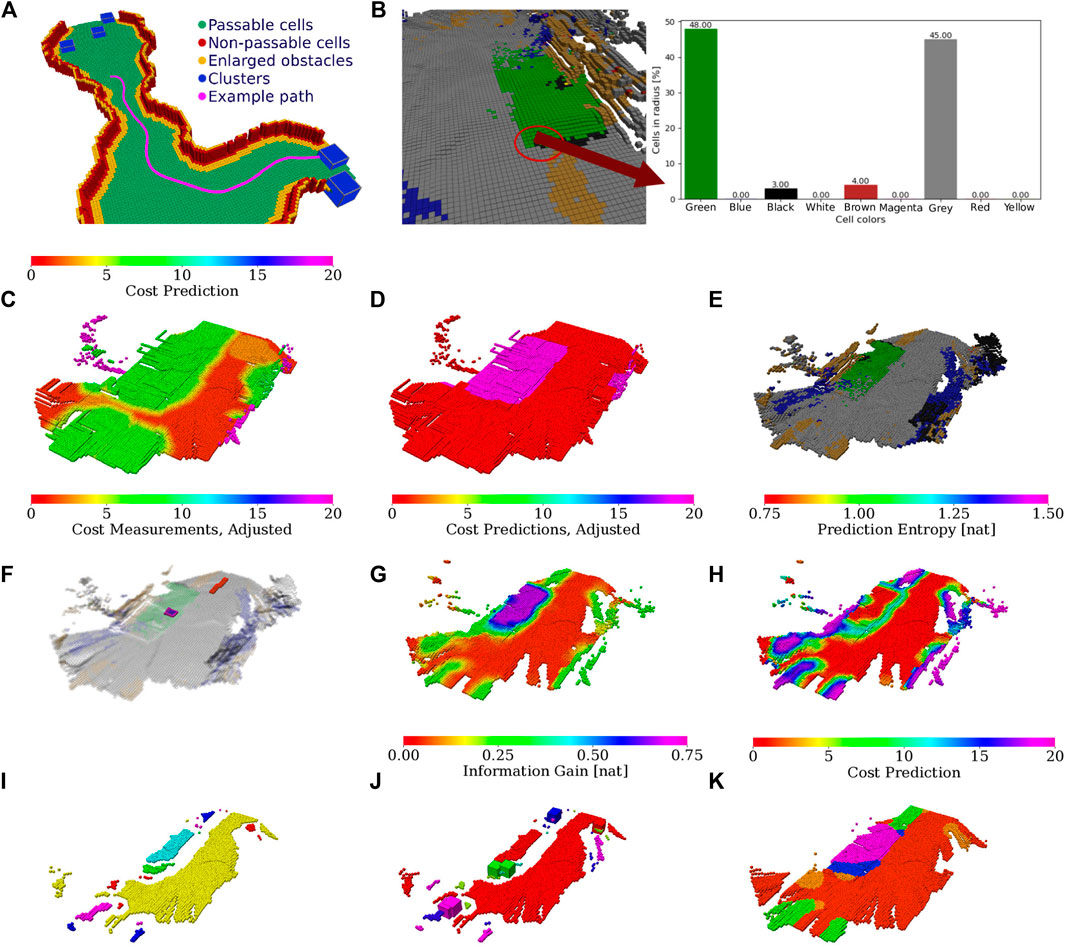
FIGURE 5. Illustration of the color-geometric and cost models. (A) Visualization of the online built geometrical model with marked passability and clusters based on the cells with non-zero information according to the shown color legend; (B) terrain appearance descriptor calculated as a histogram of cell colors. The costs used in path planning; (C) minimal cost over gaits after the distance transform; (D) respective cheapest gait (gaits in red and purple). (E) Colors used to build the color histogram terrain appearance descriptor; (F) measured costs used for learning the GP (adjusted by hyperbolic tangent), visualized over the terrain appearance; (G) raw GP cost prediction; (H) GP prediction uncertainty. (I) Terrain clusters (arbitrary colors used to distinguish clusters); (J) information gained with terrain learning goals (goal colors corresponding to clusters); (K) cluster costs used in planning.
Algorithm 3. Cluster entropy representatives
In addition to the terrain geometry, the grid map
4.3 Traversal cost model
The cost model
where δ(r, ν) lists all cells within the r-radius of cell ν, and
The cost
where each gait-terrain cost
Algorithm 4. Navigate
The cost prediction (visualized in Figure 5G) is the expected value.
and the uncertainty of the prediction (shown in Figure 5H) is characterized by the differential entropy.
The prediction uncertainty is used to approximate the information gain
where ta(T) is the appearance assigned to the terrain class
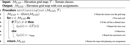
where the maximum cost cmax is reported for cells with no class (i.e., eroded) ∅.The rest of this section describes how the traversal cost experience used to learn the models is measured, how the GP regressor is learned, and how the terrain type clustering is used to identify the locations where to improve the cost model.
4.3.1 Traversal cost measurement
The measured traversal cost describes the time needed to traverse between cells as zc (ν, ν′). Since the distance between 2 cells is significantly lower than the robot stride length, the cost is smoothed over path segments (cell sequences) with a fixed duration. In particular, the per-meter cost c is continually measured as the inverted robot velocity v−1 over the path segment traversed by the robot in the last Δ t s.
where ‖ψs‖ is the length of the segment in meters and T(ψ) is the measurement duration that is fixed to Δt. If the robot had not changed its gait on the segment, the cost is reported to the particular model
where the maximum robot velocity vmax (maximum from all
4.3.2 Gaussian process traversal cost regressor
The employed GP regressor predicts both the prediction mean and variance making it suitable to model the prediction distribution as in (Eq. 14). Its description is dedicated to Supplementary Appendix S2 to make the study self-contained. GP regressor is learned only if there are at least
Algorithm 5. Traversal cost model learning.

The covariance function used in this work is the squared exponential kernel.
where
where
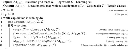
4.3.3 Terrain type clustering and goal identification
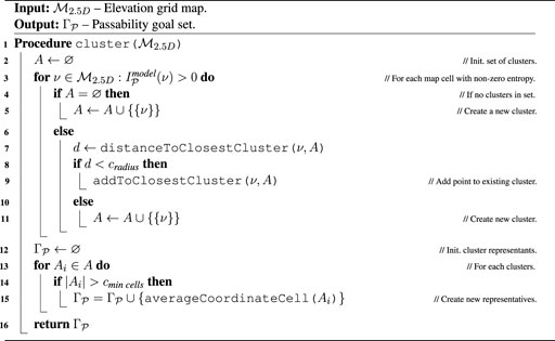
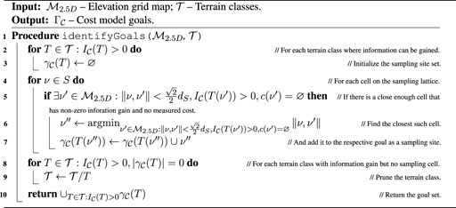
The traversal cost exploration goals
Algorithm 6. Terrain type clustering, goal identification, and cost identification.
Algorithm 7. Cluster.
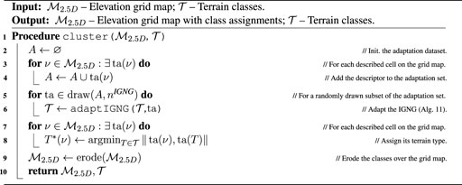
The clustering scheme presented in Algorithm 7 is based on the IGNG, described in Supplementary Algorithm S1, to make the study self-contained. In the neural gas, each neuron is a terrain prototype ta(T) in the descriptor space that represents a terrain class T. When separating the classes, the intuition is that for exponential kernels, the length scale describes the range from the data where the model can reliably extrapolate, as used, for example, in Karolj et al. (2020). Hence, new classes are inserted into the neural gas when the distance from all prototypes exceeds σIGNG = 2l. The neural gas is constructed incrementally by repeated adaptation using the appearance descriptors in the environment, where the size of each adaptation batch is limited to nIGNG descriptors that are randomly sampled from all the descriptors, and the yielded terrain classes can be seen in Figure 5I.
Algorithm 8. Compute information gain.
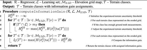
The terrain classes for which the cost model can be improved are identified using the cost regressor
where
where we avoid overconfident GP-predictions for barely sampled terrains by allowing only terrain classes with at least mT observed ground truth cost values. The threshold equals the maximum value over such ground truth terrain classes.
Algorithm 9. Identify goals.
The sampling locations (visualized, for example, in Figure 5J) corresponding to the terrain class are sampled along a lattice S with the cell size dS ≫ dν, as depicted in Algorithm 9. For each lattice point pS, the closest cell ν in
Algorithm 10. Set planning cost.
5 Experimental evaluation
The proposed exploration with active terrain learning has been examined in simulated trials and real experimental deployments using a hexapod walking robot. The simulated and real scenarios have been set up so that the robot first explores the environment and learns the cost models using the proposed method and, in some tests, a selected baseline method. Then the performance has been evaluated and compared with the baseline approach by navigating the robot over a sequence of benchmark waypoints using the respective traversal cost models of the environment learned during the exploration.
The hexapod walking robot, which can be seen in Figure 1, is used in the real deployment, and the simulation is parameterized to mimic the robot’s motion and sensory capabilities. The robot has six legs, each comprising three Dynamixel XM430-W350 servomotors. The robot is equipped with the Intel RealSense D435 camera used to construct the colored environment model and the Intel RealSense T265 localization camera. The onboard computation is provided by the Intel NUC 10i7FNK with Intel Core i7 10710U accompanied with 64 GB memory, running Ubuntu 18.04 with ROS Melodic (Quigley et al., 2009). The robot locomotion is facilitated by a blind adaptive motion gait (Faigl and Čížek, 2019). The robot uses two particular gait configurations, see Table 2: The fast gait suitable for flat, even surfaces, and the tall gait that performs better than the fast gait over rough terrain but otherwise is slower. The robot is equipped with a reflex that detects that the robot is stuck with costs exceeding cmax and switches over to the tall for Δtfallback seconds to avoid the robot getting stuck when using the baseline model or at the beginning of the learning process. The parameterization of the proposed method can be found in Table 3, and the operating frequencies of the proposed method’s processes are depicted in Table 4.
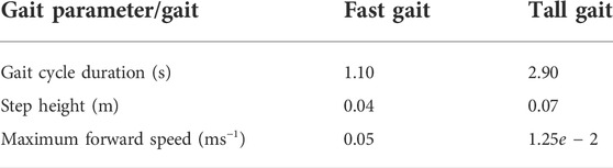
TABLE 2. Gait parameterization.
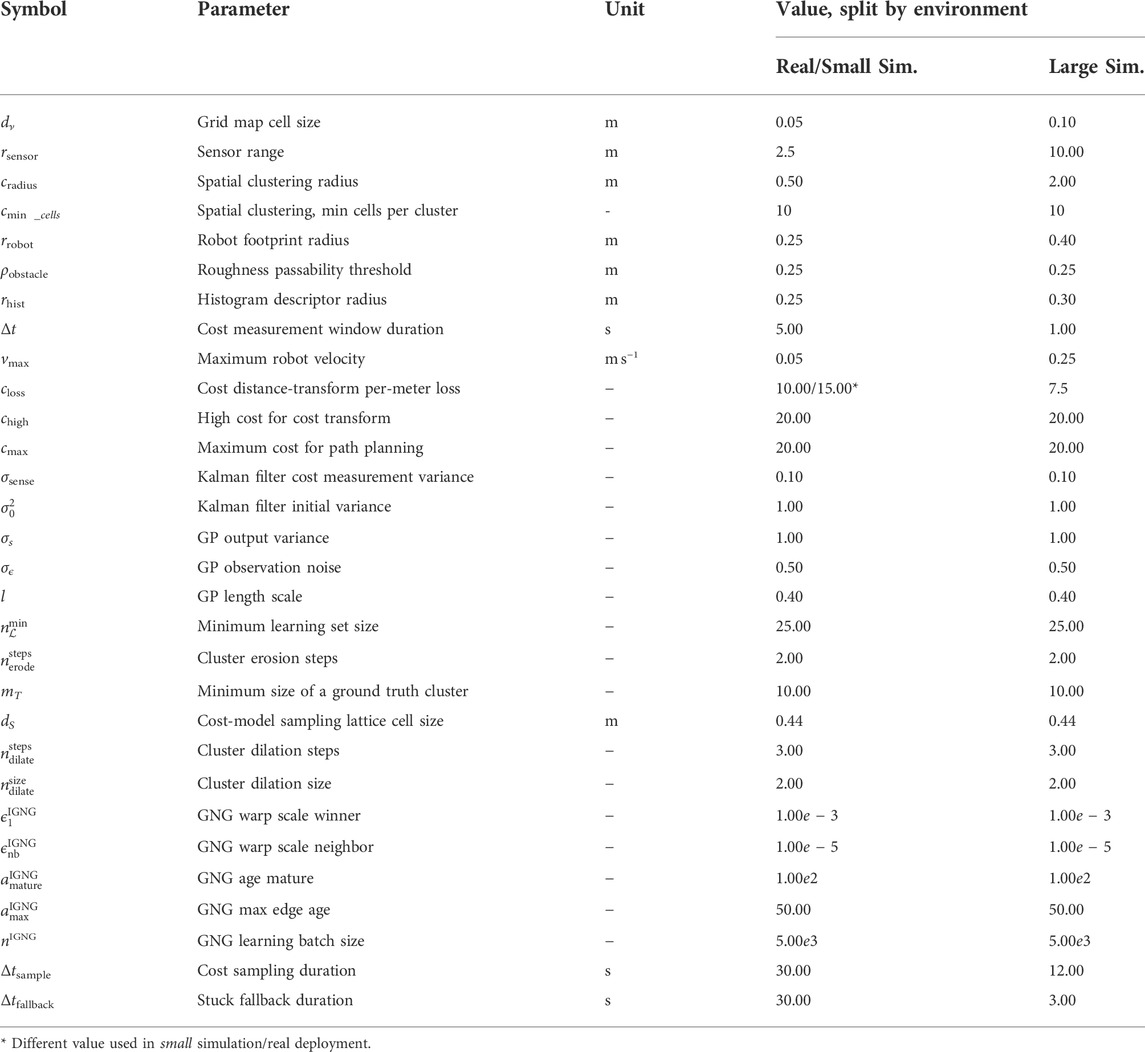
TABLE 3. System parameterization.
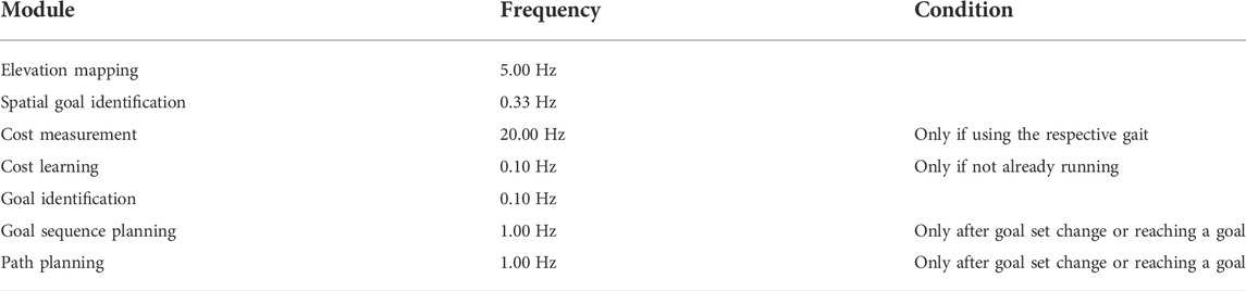
TABLE 4. System operation frequencies.
5.1 Simulated scenarios
The simulated scenarios are based on a courtyard environment captured by four 3D scans obtained using Leica BLK 360 3D scanner and visualized in Figure 6A. The scanner has standard deviation of 4 mm at 10 m and 7 mm at 20 m. The scans total approx. 1.4×10⁸ points.
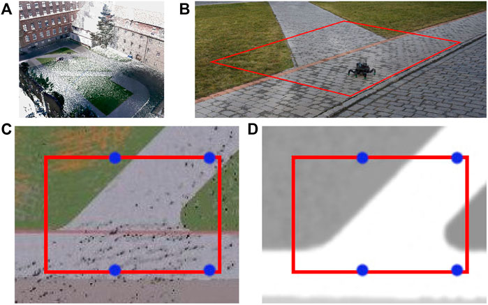
FIGURE 6. (A) 3D scan of the university campus at Charles Square in Prague, (B) section of the courtyard, and the respective simulated environment (C) color and (D) relative traversability (light areas easier to traverse). The red bounding box represents the area where the robot should explore. The blue points are the points to be visited by the robot in the first test tour.
In total, two virtual environments are created using the scan: small and large. The small environment represents a small section of the courtyard, where the simulated robot mimics the real robot’s speed and sensory equipment. It is used to test the benefit of the individual components of the proposed approach by comparing them to baseline methods where the particular component is removed or simplified. The large environment comprises terrain segments observed in the scan that are rearranged to create a larger, artificial environment with obstacles where different exploration algorithms are compared using a faster robot with an extended sensor range.
5.1.1 Small environment
The small environment is concerned with a section of the environment that is detailed in Figure 6B. We have created a simulation model of the environment containing several types of pavement (gray and red) and turf (green, brown), shown in Figure 6C. The turf is modeled as hard to traverse and can get the robot stuck for the fast gait, whereas the pavement does not impede the robot, see Figure 6D.
First, to demonstrate the benefits of using a cost model learned from prior experience, the robot is tasked to execute two tours in the environment using the learned cost model and a flat-cost baseline model. Second, the utility of exploring along the proposed GTSP-derived path is demonstrated by comparing its time to explore the environment with a greedy, myopic baseline, which drives the robot to the cheapest goal to reach w.r.t. the so far learned costs.
The first tour comprises four waypoints. The robot starts at the bottom-left point and executes the tour counter-clockwise until reaching the start location again. The two particular areas are designed to demonstrate the utility of the learned model: 1) the segment between the bottom-right and top-right waypoints where the robot can choose either a direct route over the turf or a longer path over the pavement and 2) the area around the top-left waypoint where the turf cannot be avoided and thus the robot needs to switch to the tall gait. The second tour comprises 20 points randomly sampled in the environment, and it serves to demonstrate the performance of the learned model over a tour that was not handcrafted.
In addition to the proposed approach and the baseline, in the simulated tests, we also deploy a hybrid gait selection approach that chooses its gait using the proposed model but does not plan its path w.r.t. the predicted costs and walks directly to the next waypoint. Unlike the baseline approach, which switches to the tall gait when stuck and repeatedly tries to switch back to the fast gait, the hybrid gait selection approach switches gaits only when approaching or leaving the terrain identified as hard to traverse by the model. Hence, it should outperform the baseline over longer sections on difficult terrains, where the baseline is slowed down by trying to switch back to the fast gait.
The simulation environment consists of the Intel i7-9700 3.00 GHz with 32 GB memory running Ubuntu 18.04 with ROS Melodic. Since the captured environment comprises terrains that might slow down the robot because they are somewhat non-rigid, instead of using a geometry-based simulator such as Gazebo, which cannot model such terrains, we elect to build a virtual environment over a simple simulator using real-world data. The simulation is performed using the simple two dimensional robot simulator (STDR)3 within the ROS ecosystem. On top of the simulator, we have implemented an interface that simulates the robot’s RGB-D camera, which assigns each point in the robot’s simulated exteroceptive measurements color based on the point’s position in the environment color map shown in Figure 6C and filters the measurements to contain only points within the 87 deg wide field of view of the simulated RGB-D camera. The terra-mechanical properties are simulated by slowing down the robot over the individual traversed terrains w.r.t. the performance observed over such terrain in a real-world deployment, as shown in Figure 6D.
In the evaluation, the robot first explores and learns the models shown in Figure 7A to Figure 7I. An example exploration path can be seen in Figure 7J. The robot learns that the turf, which appears either green or brown, cannot be traversed by the fast gait and thus selects the tall gait over that terrain type. On the other hand, the pavement does not hinder the fast gait, which is considerably faster and thus preferred.
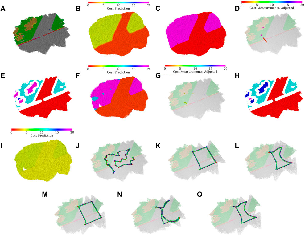
FIGURE 7. Environment assessment after the simulated scenario run with regards to both gaits; (A) dominant color in the histogram feature; (B) merged cost used for planning; (C) selected gait (fast in red, tall in purple); (D) costs used for learning the fast gait model [adjusted by hyperbolic tangent in (Eq. 20)], visualized over the terrain appearance; (E) clusters used in the fast gait model (arbitrary colors used to distinguish clusters); (F) fast gait cost predictions assigned by the dilated clusters; (G) costs used for learning the tall gait model [adjusted by hyperbolic tangent using (Eq. 20)], visualized over the terrain appearance; (H) clusters used in the tall gait model (arbitrary colors used to distinguish clusters); (I) tall gait cost predictions assigned by the dilated clusters; (J) exploration run; (K) test-tour run using the baseline model without the learned traversal costs; (L) test-tour run using the learned traversal costs. The development of the path through the fully discovered simulated environment during the exploration; (M) at the beginning of the exploration, the robot uses flat costs and thus does not avoid difficult terrains; (N) after learning the costs for the fast gait, the robot is too cautious and avoids going near the costly turf; (O) after learning the tall gait costs, the robot is less cautious and is willing to walk near difficult terrain.
Although the two gait models create the terrain clusters independently, the clusters in Figure 7E and Figure 7H differ only in cluster indices used in the internal representation (each index is associated with a different color in the visualization). It can be observed that the robot does not use any clusters associated with the red line on the pavement, either removing the thin cluster outright in the erosion or pruning the small erosion remains after the robot finds out that it cannot get enough samples to learn such a small terrain.
In the particular exploration run shown in Figure 7J, the robot first walks along the left side of the exploration bounds, learning the fast gait costs for both the pavement and turf and the tall gait cost over the turf. Then the robot learns the tall gait cost over the pavement while clearing the spatial exploration goals. During the exploration, it can be seen that the robot avoids walking over the remaining turf, only approaching it at the very end of the exploration. Thus, the robot needs only to enter and not leave the turf (minimizing the time on the costly terrain) to reach the goal that lies on the turf.
The test runs using the baseline, and the learned model over the first tour are shown in Figure 7K and Figure 7L, respectively. In addition, the development of the tours that would be used at different points during the exploration can be seen in Figure 7M through Figure 7O. In the baseline test, the robot walks directly between the waypoints and only switches to the tall gait after getting stuck. On the other hand, when using the learned model, the robot avoids the turf if possible and switches to the tall gait before entering the turf while pursuing the top-left goal.
The performance over 25 simulated trials (five exploration runs, each with five tour tests for the tour tests; 25 runs for the simulated exploration tests) can be observed in Table 5. On the first tour, the hybrid gait selection approach is slower than the reactive baseline. In the authors’ opinion, it is caused by the conservative (large) value of rrobot, which compels the robot to use the slow tall gait on the border between the rough terrain and pavement, whereas the reactive approach only tries to switch back to the fast gait (which is its main disadvantage when compared to the hybrid approach) a few times on the short rough terrain segment. Nonetheless, the proposed learned model knows to avoid such areas and performs better or the same as the other approaches over every tour segment. Hence, the results suggest that robot benefits from using the learned costs in path planning. Over the second tour, the robot performs similarly. The learned model outperforms the baseline when moving around or over the turf. Both approaches exhibit similar travel times when the direct path between the waypoint leads only over the pavement. Unlike over the first tour, the hybrid gait selection performs better than the baseline approach, presumably due to longer sections over hard-to-traverse terrains on the second tour. The proposed approach consistently outperforms the baseline and hybrid gait selection approaches; we conclude that the robot benefits from using the learned model.
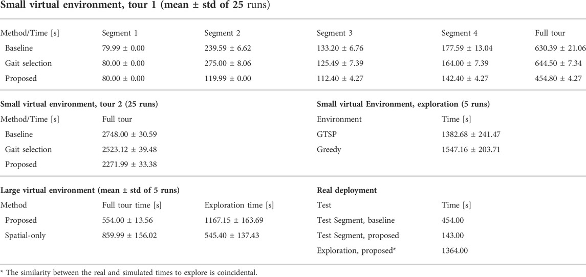
TABLE 5. Performance as the time (total cost) in seconds to traverse.
In addition to the tour tests, the results suggest that the robot benefits from using the non-myopic GTSP planner compared to the myopic greedy approach. Even though the performance of the two approaches appears relatively close, the Mann–Whitney U Test (Mann and Whitney, 1947) rejects the null hypothesis of the same exploration time distribution at 99.5% confidence against both the two-sided and the relevant one-sided alternative. In the authors’ opinion, the high variance in the observed exploration times can be attributed to the effect of random chance in exploration since neither myopic nor non-myopic approaches are informed about the terrains in unexplored areas. However, the myopic explorer is more likely to make a bad decision, such as not clearing some of the goals in a particular area that needs to be visited later. Therefore, the proposed non-myopic approach performs better overall.
5.1.2 Large environment
The large environment is an artificial 20 × 25 m outdoor/indoor scenario. The map comprises patches from the courtyard scan rearranged as shown in Figure 8. Given the size of the environment, the robot is sped up five times. The cell size is increased to 0.1 m, and other parameters are adjusted accordingly, see Table 3. In addition, the robot uses an omnidirectional sensor with the increased range of 10 m, which expands the range of terrains that can be observed without the respective terrain’s traversal. To accommodate the simulation of the increased sensor range, the virtual environment is run on AMD Ryzen Threadripper 3960× 3.8 GHz with 48 GB memory running Ubuntu 18.04 and ROS Melodic, using STDR in the same manner as for the small environment.
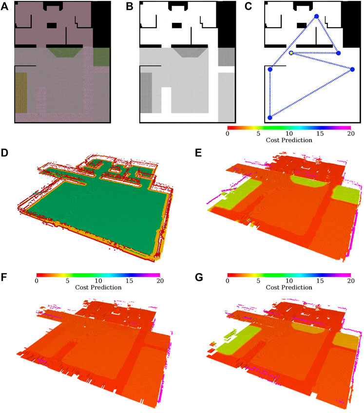
FIGURE 8. Large simulated environment (A) color and (B) relative traversability, (C) and the test tour through the environment, which starts at the starred node and is counter-clockwise. The built maps of the large simulated environment: (D) geometric map and (E) merged costs used for planning after exploration using the proposed approach; merged costs ofter exploration using the spatial-only model while (F) avoiding and (G) traversing rough terrain, respectively.
Similar to the small environment, the robot is first set to explore the environment and then is tasked to visit the set of waypoints shown in Figure 8C. The proposed algorithm is compared to a spatial-only baseline approach, which learns the cost models only as a result of experiencing cost while pursuing spatial exploration goals. The spatial-only changes the gaits in a reactive fashion when stuck and hence only learns the model for the tall gait if it enters the difficult green or brown turf during the exploration.
The quantitative results for the large environment are shown in Table 5. Since the proposed approach actively tries to sample every terrain type, it is slower to explore the whole environment. However, the proposed approach performs better in the tour evaluation. Closer examination suggests that while the tour times of the proposed approach remain similar in all trials, the spatial-only times vary wildly since the learned models differ based on which terrains the robot has traversed during the exploration. This randomness can be attributed to differences in simulation and plan execution. In addition, Figures 8D–G shows the learned maps for the proposed model, and for the spatial-only model in both the cases when the rough terrain was and was not traversed. For the case when a rough terrain was traversed by the spatial-only model, the costs differ between the individual rough areas. However, the ground truth costs shown in Figure 8B suggest that they should be the same, as is the case for the proposed model. Likely, this is caused by the robot traversing only the brown-green rough terrain located on the left of the environment. The green terrain, located in the center and right of the environment, appears somewhat similar to the brown-green terrain. Hence, the robot considers it to be difficult to traverse to a certain degree. However, since the spatial-only model does not deliberately sample the terrains, the model’s guess differs somewhat from the exact cost to traverse the particular terrain, decreasing the fidelity of the predictions.
Overall, the presented results suggest that the proposed approach presents a tradeoff in terms of exploration and execution time: the longer time spent exploring the environment and learning the cost models provides the robot with better cost maps, which shorten the time to navigate the environment after it is explored. It should be noted that since the behavior of the spatial-only model is affected by random chance (differences in simulation and plan execution), it can provide models as good as the proposed approach. However, there is no guarantee that this would happen regularly, whereas the proposed approach has returned high fidelity maps in every test case.
5.2 Real robot experimental deployment
The viability of the proposed approach is demonstrated in the real experimental deployment, where the robot explores an indoor 2 × 6 m area visualized in Figure 9. The office-like environment comprises flat synthetic terrain that is easy to traverse but appears to the robot differently colored at different locations since it is glossy and carries the color of nearby objects located next to the arena. When building the colored elevation map
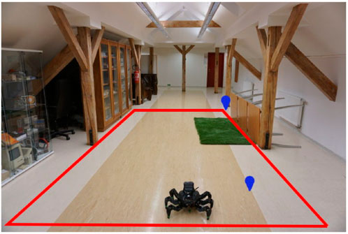
FIGURE 9. The 2m × 6m large deployment area with a green artificial turf. The area boundary is in red, and the waypoints of the test tour are depicted in blue. The shown robot is at the starting position.
Figure 10 shows the maps learned in the experimental run, which is also presented in the accompanying Supplementary Video S1. A colored map of the environment is depicted in Figure 10A. The overall costs and selected gaits through the environment are shown in Figure 10B and Figure 10C, respectively.
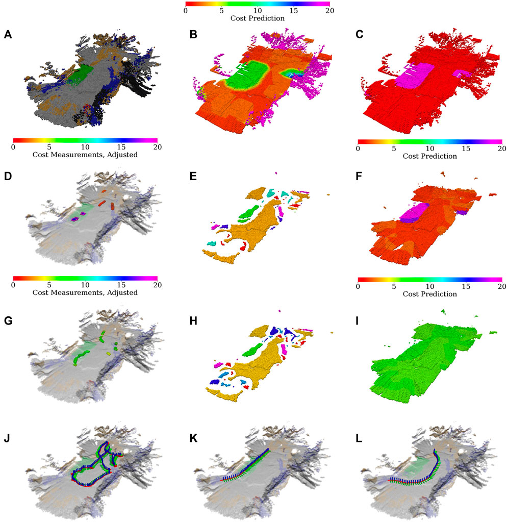
FIGURE 10. Environment evaluation and the real robot exploration run; (A) dominant color in the histogram feature; (B) merged cost used for planning; (C) selected gait (fast in red, tall in purple); (D) costs used for learning the fast gait model (adjusted by hyperbolic tangents), visualized over the terrain appearance; (E) clusters used in the fast gait model (arbitrary colors used to distinguish clusters); (F) fast gait cost predictions assigned by the dilated clusters; (G) costs used for learning the tall gait model (adjusted by hyperbolic tangents), visualized over the terrain appearance; (H) clusters used in the tall gait model (arbitrary colors used to distinguish clusters); (I) tall gait cost predictions assigned by the dilated clusters; (J) exploration run; (K) test-tour run using the baseline model without the learned traversal costs; (L) test-tour run using the learned traversal costs.
During the experimental deployment, the robot first learns the largest gray appearing flat terrain using the fast gait. Then it learns on the turf for both gaits and returns to the gray area to learn for the tall gait. Afterward, the robot pursues the yet unvisited spatial goals and smaller off-color terrain clusters that appear near the environment boundary and are caused by the glossy floor that carries the color of the nearby objects.
Compared to the simulation, the robot needs a larger amount of the measurements to learn the terrains (see Figure 10D and Figure 10G), and there are more terrain clusters (see Figure 10E and Figure 10H). It suggests that the real environment is noisier and contains multiple differently colored areas, which is in line with our observations regarding the glossy floor material. Nevertheless, the traversal costs learned by the robot for the individual gaits (see Figure 10F and Figure 10I) are within expectations, as is the overall planning cost depicted in Figure 10B and gait selection visualized in Figure 10C.
The test run scenarios are set up similarly to the tours used in the simulated test; the robot is placed in front of the hard-to-traverse turf and tasked to reach a goal location behind the hard-to-traverse terrain, slightly out of the exploration bounds, see Figure 9. The paths shown in Figure 10K and Figure 10L show that when using the baseline without the learned model, the robot tries to reach the goal directly over the turf, gets stuck, and needs to switch to the slow tall gait. On the other hand, when using the learned model, the robot avoids the hard-to-traverse areas and reaches its goal quickly using the fast gait. The performance in the presented run can be seen in Table 5. Overall, we conclude that the real deployment confirms that the robot can actively learn the traversability as a part of the exploration mission and benefits from using such learned models.
6 Discussion
The presented exploration system is proposed as a combination of spatial geometric modeling and learning terrain-gait traversal cost models. However, the system is designed to support additional models that do not describe the robot’s traversal cost. Moreover, since the models are kept separate, there is no need to use the same feature set for each of them. Therefore, the approach is compatible with spatial models such as magnetism models (Karolj et al., 2020) or GP-based occupancy (Wang and Englot, 2016). The only requirement for a model is that it produces a set of learning goals in the environment that are resolved once particular information is sampled. Hence, the proposed system can be extended by including additional traversability models, such as modeling the passability of potentially non-rigid obstacles.
In addition, we approach the traversal cost prediction so that it supports any cost model that is additive along the traversed path, such as time to traverse or consumed energy. Besides, individual cost predictors describe the gaits of a hexapod walking robot, but they can also describe any discrete set of robot configurations. Hence, the approach is viable for any mobile robot that describes its motion experience using an additive cost and can also be used to model the energy a tracked robot consumes, for example, with adjustable flippers. A particular limitation of the cost modeling used in the presented approach is that we assume that the individual gaits are switched for free w.r.t. the cost (i.e., instantaneously for cost modeled as the time to traverse), whereas in practice, the gait requires some time to exhibit its properties. In this study, we leave the question of how to predict gait-change cost open for future work.
The used cost model goal generation stems from the idea that adding new observations does not increase GP uncertainty if the hyper-parameters are fixed (Rasmussen and Williams, 2006). Therefore, sampling new measurements should not increase uncertainty and thus not spawn new goals in areas containing none. In practice, even though we use fixed GP hyper-parameters, the non-increasing nature of the uncertainty does not strictly hold for the approximated information gain since, in addition to the GP hyper-parameters, the information gain also depends on the terrain clusters and the costs and descriptors in the learning set, all of which might drift during the exploration. However, the robot behavior demonstrated in both evaluation setups shown in Figure 7J and Figure 10J suggests that the assumption holds in general. The robot clears the areas corresponding to the individual terrains (goals) and is not compelled to return to previously visited areas.
The primary limitation of the proposed approach is identified in its inability to compare the utility of the goals originating from the different models. We are motivated to build a modular system that would support different model types; therefore, the proposed decoupled approach considers each goal equally valued, regardless of the source model. This limits how the models are used since the goal utility, such as the information gain, is relegated to be used only inside the particular model to determine which environment features (locations or terrain types) are goals to use in creating an instance of the GTSP. The proposed approach provides a non-myopic solution to visit the goals reported by the individual models, where the models are also non-myopic since each can report multiple goals. Myopic models that would report their respective highest utility goal (potentially with multiple sampling sites) can be used. However, similarly to the myopic planner with the results reported in Table 5, the time to explore would likely increase since the GTSP planner would lack the information on where to go after the current goals are sampled, and thus the exploration path would often change significantly. Integrating goal utility into the decoupled planning and using alternative utility functions such as the GP-UCB remains the subject of future work.
7 Conclusion
In this study, we present a system for autonomous mobile robot exploration that incorporates active learning of traversal cost models in addition to spatial model building. During the exploration, the robot builds the spatial geometric model of the environment and learns the traversal cost models, each comprising a Gaussian process regressor and a growing neural gas terrain clustering scheme. The geometric model is used to determine areas passable by the robot, while the cost models predict the traversal costs over the passable terrains from the terrain’s appearance. Each cost model corresponds to a particular hexapod walking robot locomotion gait. The robot approaches exploration in a decoupled manner, creating a set of goals for the spatial exploration and for each traversal cost model. The exploration path is planned by solving an instance of the generalized traveling salesman problem over the goals that are sets of possible sites of visits to improve the particular model. The proposed system has been evaluated in simulation setup and real experimental deployment with two different walking gaits. The results suggest that the proposed system yields the robot to explore the environment and learn the traversal cost models. The learned models benefit the robot’s operation in the environment. In future work, we plan to model the gait change costs, include additional traversability models such as obstacle rigidity, and extend the proposed approach to support goal utility and exploration–exploitation models.
Data availability statement
The raw data supporting the conclusion of this article will be made available by the authors, without undue reservation.
Author contributions
With the support of JF, MP, and JB designed the proposed system. MP and JB performed the experiments and processed the data. MP, JB, and JF wrote the manuscript. All the authors contributed to the manuscript and approved the submitted version.
Funding
The work was supported by the Czech Science Foundation (GAČR) under research project No. 18-18858S and 19-20238S. The support under the OP VVV funded project CZ.02.1.01/0.0/0.0/16_019/0000765 “Research Center for Informatics” is also gratefully acknowledged.
Acknowledgments
We would like to thank Petr Čížek and Jiří Kubík for their help with the hexapod walking robot maintenance.
Conflict of interest
The authors declare that the research was conducted in the absence of any commercial or financial relationships that could be construed as a potential conflict of interest.
Publisher’s note
All claims expressed in this article are solely those of the authors and do not necessarily represent those of their affiliated organizations, or those of the publisher, the editors, and the reviewers. Any product that may be evaluated in this article, or claim that may be made by its manufacturer, is not guaranteed or endorsed by the publisher.
Supplementary material
The Supplementary Material for this article can be found online at: https://www.frontiersin.org/articles/10.3389/frobt.2022.910113/full#supplementary-material
Footnotes
1In the simulated experiments, the localization is provided by the simulator.
2In practice, for small environments, it is feasible to compute the prediction for every cell, and we do so for visualization as depicted in Figure 5G and Figure 5H.
3http://stdr-simulator-ros-pkg.github.io
References
Azpúrna, H., Campos, M. F. M., and Macharet, D. G. (2021). Three-dimensional terrain aware autonomous exploration for subterranean and confined spaces. IEEE Int. Conf. Robotics Automation (ICRA), 2443. –2449. doi:10.1109/ICRA48506.2021.9561099
Baleia, J., Santana, P., and Barata, J. (2015). On exploiting haptic cues for self-supervised learning of depth-based robot navigation affordances. J. Intell. Robot. Syst. 80, 455–474. doi:10.1007/s10846-015-0184-4
Bayer, J., and Faigl, J. (2021). “Decentralized topological mapping for multi-robot autonomous exploration under low-bandwidth communication,” in European Conference on Mobile Robots (Bonn, Germany: ECMR), 1–7. doi:10.1109/ECMR50962.2021.9568824
Bayer, J., and Faigl, J. (2019). “Speeded up elevation map for exploration of large-scale subterranean environments,” In 2019 Modelling and Simulation for Autonomous Systems (Palermo, Italy: MESAS), 192–202. doi:10.1007/978-3-030-43890-615
Bayer, J., and Faigl, J. (2020). “Speeded up elevation map for exploration of large-scale subterranean environments,” in 2020 Modelling and Simulation for autonomous systems (MESAS). 190–202.
Bekhti, M. A., and Kobayashi, Y. (2016). “Prediction of vibrations as a measure of terrain traversability in outdoor structured and natural environments,” in Image and video technology, 282–294. doi:10.1007/978-3-319-29451-3_23
Belter, D., Wietrzykowski, J., and Skrzypczyński, P. (2019). Employing natural terrain semantics in motion planning for a multi-legged robot. J. Intell. Robot. Syst. 93, 723–743. doi:10.1007/s10846-018-0865-x
Binney, J., and Sukhatme, G. S. (2012). Branch and bound for informative path planning. IEEE Int. Conf. Robotics Automation (ICRA), 2147. –2154. doi:10.1109/ICRA.2012.6224902
Bourgault, F., Makarenko, A. A., Williams, S. B., Grocholsky, B., and Durrant-Whyte, H. F. (2002). “Information based adaptive robotic exploration,” in IEEE/RSJ international conference on intelligent robots and systems (Lausanne, Switzerland: IROS), 540–545. doi:10.1109/IRDS.2002.1041446
Bradley, D. M., Chang, J. K., Silver, D., Powers, M., Herman, H., Rander, P., et al. (2015). “Scene understanding for a high-mobility walking robot,” in IEEE/RSJ international conference on intelligent robots and systems (Hamburg, Germany: IROS), 1144–1151. doi:10.1109/IROS.2015.7353514
Brown, D., and Webster, G. (2010). Now a stationary research platform, NASA’s Mars rover Spirit starts a new chapter in red planet scientific studies. Pasadena, CA: NASA Press Release.
Carrillo, H., Dames, P., Kumar, V., and Castellanos, J. A. (2018). Autonomous robotic exploration using a utility function based on Rényi’s general theory of entropy. Auton. Robots 42, 235–256. doi:10.1007/s10514-017-9662-9
Charrow, B., Liu, S., Kumar, V., and Michael, N. (2015). Information-theoretic mapping using cauchy-schwarz quadratic mutual information. IEEE Int. Conf. Robotics Automation (ICRA), 4791–4798. doi:10.1109/ICRA.2015.7139865
Dang, T., Tranzatto, M., Khattak, S., Mascarich, F., Alexis, K., and Hutter, M. (2020). Graph-based subterranean exploration path planning using aerial and legged robots. J. Field Robot. 37, 1363–1388. doi:10.1002/rob.21993
Faigl, J., and Čížek, P. (2019). Adaptive locomotion control of hexapod walking robot for traversing rough terrains with position feedback only. Robotics Aut. Syst. 116, 136–147. doi:10.1016/j.robot.2019.03.008
Faigl, J., and Kulich, M. (2013). “On determination of goal candidates in frontier-based multi-robot exploration,” in European conference on mobile robots (Barcelona, Spain: ECMR), 210–215. doi:10.1109/ECMR.2013.6698844
Faigl, J., Kulich, M., and Přeučil, L. (2012). “Goal assignment using distance cost in multi-robot exploration,” in IEEE/RSJ international conference on intelligent robots and systems (Vilamoura-Algarve, Portugal: IROS), 3741–3746. doi:10.1109/IROS.2012.6385660
Fankhauser, P., Bloesch, M., Gehring, C., Hutter, M., and Siegwart, R. (2014). World Scientific, 433–440.Robot-centric elevation mapping with uncertainty estimatesMob. Serv. Robot.
Forouhar, M., Čížek, P., and Faigl, J. (2021). “Scarab II: A small versatile six-legged walking robot,” in 5th full-day workshop on legged robots at IEEE international conference on robotics and automation (Xi’an, China: ICRA), 1–2.
Fritzke, B. (1994). “A growing neural gas network learns topologies,” in Conference on neural information processing systems (Denver, CO: NIPS), 625–632.
Gonzalez, R., and Iagnemma, K. (2018). Slippage estimation and compensation for planetary exploration rovers. State of the art and future challenges. J. Field Robotics 35, 564–577. doi:10.1002/rob.21761
Guastella, D. C., and Muscato, G. (2021). Learning-based methods of perception and navigation for ground vehicles in unstructured environments: A review. Sensors 21, 73. doi:10.3390/s21010073
Guerrero, E., Bonin-Font, F., and Oliver, G. (2021). Adaptive visual information gathering for autonomous exploration of underwater environments. IEEE Access 9, 136487–136506. doi:10.1109/ACCESS.2021.3117343
Haddeler, G., Chan, J., You, Y., Verma, S., Adiwahono, A. H., and Meng Chew, C. (2020). “Explore bravely: Wheeled-legged robots traverse in unknown rough environment,” in IEEE/RSJ international conference on intelligent robots and systems (Las Vegas, NV: IROS), 7521–7526. doi:10.1109/IROS45743.2020.9341610
Helsgaun, K. (2000). An effective implementation of the lin-kernighan traveling salesman heuristic. Eur. J. Operational Res. 126, 106–130. doi:10.1016/s0377-2217(99)00284-2
Hollinger, G. A., and Sukhatme, G. S. (2014). Sampling-based robotic information gathering algorithms. Int. J. Rob. Res. 33, 1271–1287. doi:10.1177/0278364914533443
Homberger, T., Bjelonic, M., Kottege, N., and Borges, P. V. K. (2016). “Terrain-dependant control of hexapod robots using vision,” in International symposium on experimental robotics (Nagasaki, Japan: ISER), 92–102. doi:10.1007/978-3-319-50115-4_9
Karolj, V., Viseras, A., Merino, L., and Shutin, D. (2020). An integrated strategy for autonomous exploration of spatial processes in unknown environments. Sensors 20, 3663. doi:10.3390/s20133663
Kottege, N., Parkinson, C., Moghadam, P., Elfes, A., and Singh, S. P. N. (2015). Energetics-informed hexapod gait transitions across terrains. IEEE Int. Conf. Robotics Automation (ICRA), 5140–5147. doi:10.1109/ICRA.2015.7139915
Krajník, T., Fentanes, J. P., Santos, J. M., and Duckett, T. (2017). Fremen: Frequency map enhancement for long-term mobile robot autonomy in changing environments. IEEE Trans. Robot. 33, 964–977. doi:10.1109/TRO.2017.2665664
Krüsi, P., Bosse, M., and Siegwart, R. (2016). Driving on point clouds: Motion planning, trajectory optimization, and terrain assessment in generic nonplanar environments. J. Field Robot. 34, 940–984. doi:10.1002/rob.21700
Lin, B., and Song, S. (1993). Dynamic modeling, stability and energy efficiency of a quadrupedal walking machine. J. Robot. Syst. 18, 657–670. doi:10.1002/rob.8104
Luo, W., and Sycara, K. (2018). Adaptive sampling and online learning in multi-robot sensor coverage with mixture of Gaussian processes. IEEE Int. Conf. Robotics Automation (ICRA), 6359–6364. doi:10.1109/ICRA.2018.8460473
Ma, K.-C., Liu, L., Heidarsson, H. K., and Sukhatme, G. S. (2018). Data-driven learning and planning for environmental sampling. J. Field Robot. 35, 643–661. doi:10.1002/rob.21767
Makarenko, A. A., Williams, S. B., Bourgault, F., and Durrant-Whyte, H. F. (2002). in IEEE/RSJ international conference on intelligent robots and systems, 1, An experiment in integrated exploration534–539. doi:10.1109/IRDS.2002.1041445(IROS)
Mann, H. B., and Whitney, D. R. (1947). On a test of whether one of two random variables is stochastically larger than the other. Ann. Math. Stat. 18, 50–60. doi:10.1214/aoms/1177730491
Martin, S., and Corke, P. (2014). Long-term exploration & tours for energy constrained robots with online proprioceptive traversability estimation. IEEE Int. Conf. Robotics Automation (ICRA), 5778–5785. doi:10.1109/ICRA.2014.6907708
Mayuku, O., Surgenor, B. W., and Marshall, J. A. (2021). “A self-supervised near-to-far approach for terrain-adaptive off-road autonomous driving,” in IEEE international conference on robotics and automation (Xi’an, China: ICRA), 14054–14060. doi:10.1109/ICRA48506.2021.9562029
McGhee, R. B., and Frank, A. A. (1968). On the stability properties of quadruped creeping gaits. Math. Biosci. 3, 331–351. doi:10.1016/0025-5564(68)90090-4
Moravec, H., and Elfes, A. (1985). “High resolution maps from wide angle sonar,” in 1985 IEEE international conference on robotics and automation proceedings, 116–121. doi:10.1109/ROBOT.1985.1087316
Noon, C. E., and Bean, J. C. (1993). An efficient transformation of the generalized traveling salesman problem. INFOR Inf. Syst. Operational Res. 31, 39–44. doi:10.1080/03155986.1993.11732212
Noon, C. E. (1988). The generalized traveling salesman problem. Ann Arbor, MI: Ph.D. thesis, University of Michigan.
O’Callaghan, S., Ramos, F. T., and Durrant-Whyte, H. (2009). Contextual occupancy maps using Gaussian processes. IEEE Int. Conf. Robotics Automation (ICRA), 1054–1060. doi:10.1109/ROBOT.2009.5152754
O’Meadhra, C., Tabib, W., and Michael, N. (2019). Variable resolution occupancy mapping using Gaussian mixture models. IEEE Robot. Autom. Lett. 4, 2015–2022. doi:10.1109/LRA.2018.2889348
Ossenkopf, M., Castro, G., Pessacg, F., Geihs, K., and De Cristóforis, P. (2019). “Long-Horizon Active SLAM system for multi-agent coordinated exploration,” in European conference on mobile robots (Prague, Czech Republic: ECMR), 1–6. doi:10.1109/ECMR.2019.8870952
Papadakis, P. (2013). Terrain traversability analysis methods for unmanned ground vehicles: A survey. Eng. Appl. Artif. Intell. 26, 1373–1385. doi:10.1016/j.engappai.2013.01.006
Pasolli, E., and Melgani, F. (2011). Gaussian process regression within an active learning scheme. IEEE Int. Geoscience Remote Sens. Symposium, 3574–3577. doi:10.1109/IGARSS.2011.6049994
Prágr, M., Čížek, P., Bayer, J., and Faigl, J. (2019a). “Online incremental learning of the terrain traversal cost in autonomous exploration,” in Robotics: Science and systems, (RSS) (Freiburg im Breisgau, Germany). 1–10. doi:10.15607/RSS.2019.XV.040
Prágr, M., Čížek, P., and Faigl, J. (2018). “Cost of transport estimation for legged robot based on terrain features inference from aerial scan,” in IEEE/RSJ international conference on intelligent robots and systems (IROS) (Prague, Czech Republic: IEEE), 1745–1750. doi:10.1109/IROS.2018.8593374
Prágr, M., Čížek, P., and Faigl, J. (2019b). “Incremental learning of traversability cost for aerial reconnaissance support to ground units,” in 2018 modelling and simulation for autonomous systems (Prague, Czech Republic: MESAS), 412–421. doi:10.1007/978-3-030-14984-0_30
Prudent, Y., and Ennaji, A. (2005). An incremental growing neural gas learns topologies. Int. Jt. Conf. Neural Netw. (IJCNN) 2, 1211–1216. doi:10.1109/IJCNN.2005.1556026
Quann, M., Ojeda, L., Smith, W., Rizzo, D., Castanier, M., and Barton, K. (2020). Off-road ground robot path energy cost prediction through probabilistic spatial mapping. J. Field Robot. 37, 421–439. doi:10.1002/rob.21927
Quigley, M., Conley, K., Gerkey, B. P., Faust, J., Foote, T., Leibs, J., et al. (2009). ICRA Workshop on Open Source Software, 1–6.Ros: An open-source robot operating system.
Ramos, F., and Ott, L. (2016). Hilbert maps: Scalable continuous occupancy mapping with stochastic gradient descent. Int. J. Rob. Res. 35, 1717–1730. doi:10.1177/0278364916684382
Rasmussen, C. E., and Williams, C. K. I. (2006). Gaussian processes for machine learning. Adaptive computation and machine learning. Cambridge, Mass: MIT Press.
Rényi, A. (1961). On measures of entropy and information. Berkeley Symposium Math. Statistics Probab., 547–561.
Rhodes, C., Liu, C., and Chen, W.-H. (2020). “Informative path planning for gas distribution mapping in cluttered environments,” in IEEE/RSJ international conference on intelligent robots and systems (Las Vegas, NV: IROS), 6726–6732. doi:10.1109/IROS45743.2020.9341781
Schultz, A. C., Adams, W., and Yamauchi, B. (1999). Integrating exploration, localization, navigation and planning with a common representation. Auton. Robots 6, 293–308. doi:10.1023/A:1008936413435
Shi, Y., Wang, N., Zheng, J., Zhang, Y., Yi, S., Luo, W., et al. (2020). “Adaptive informative sampling with environment partitioning for heterogeneous multi-robot systems,” in IEEE/RSJ international conference on intelligent robots and systems (Las Vegas, NV: IROS), 11718–11723. doi:10.1109/IROS45743.2020.9341711
Singh, A., Krause, A., Guestrin, C., Kaiser, W., and Batalin, M. (2007). “Efficient planning of informative paths for multiple robots,” in International joint conference on artifical intelligence, 2204–2211.
Sofman, B., Lin, E., Bagnell, J. A., Cole, J., Vandapel, N., and Stentz, A. (2006). Improving robot navigation through self-supervised online learning. J. Field Robot. 23, 1059–1075. doi:10.1002/rob.20169
Srinivas, N., Krause, A., Kakade, S., and Seeger, M. (2010). “Gaussian process optimization in the bandit setting: No regret and experimental design,” in Intl. Conf. International conference on machine learning (ICML) (Haifa, Israel, 1015–1022.
Stachniss, C., Grisetti, G., and Burgard, W. (2005). “Information gain-based exploration using rao-blackwellized particle filters,” in Robotics: Science and systems, 1–8. doi:10.15607/RSS.2005.I.009
Stelzer, A., Hirschmüller, H., and Görner, M. (2012). Stereo-vision-based navigation of a six-legged walking robot in unknown rough terrain. Int. J. Rob. Res. 31, 381–402. doi:10.1177/0278364911435161
Vallvé, J., and Andrade-Cetto, J. (2015). Potential information fields for mobile robot exploration. Robotics Aut. Syst. 69, 68–79. doi:10.1016/j.robot.2014.08.009
Viseras, A., Shutin, D., and Merino, L. (2019). Robotic active information gathering for spatial field reconstruction with rapidly-exploring random trees and online learning of Gaussian processes. Sensors 19, 1016. doi:10.3390/s19051016
Wang, J., and Englot, B. (2016). Fast, accurate Gaussian process occupancy maps via test-data octrees and nested Bayesian fusion. IEEE Int. Conf. Robotics Automation (ICRA), 1003–1010. doi:10.1109/ICRA.2016.7487232
Wermelinger, M., Fankhauser, P., Diethelm, R., Krüsi, P., Siegwart, R., and Hutter, M. (2016). “Navigation planning for legged robots in challenging terrain,” in IEEE/RSJ international conference on intelligent robots and systems, 1184–1189. doi:10.1109/IROS.2016.7759199
Yamauchi, B. (1997). A frontier-based approach for autonomous exploration. CIRA (IEEE), 146–151. doi:10.1109/CIRA.1997.613851
Keywords: mobile robot exploration, active learning, traversability, multi-legged robot, locomotion gait
Citation: Prágr M, Bayer J and Faigl J (2022) Autonomous robotic exploration with simultaneous environment and traversability models learning. Front. Robot. AI 9:910113. doi: 10.3389/frobt.2022.910113
Received: 31 March 2022; Accepted: 23 August 2022;
Published: 05 October 2022.
Edited by:
Luis Rodolfo Garcia Carrillo, New Mexico State University, United StatesReviewed by:
Arturo Gil Aparicio, Miguel Hernández University of Elche, SpainHengameh Mirhajianmoghadam, New Mexico State University, United States
Copyright © 2022 Prágr, Bayer and Faigl. This is an open-access article distributed under the terms of the Creative Commons Attribution License (CC BY). The use, distribution or reproduction in other forums is permitted, provided the original author(s) and the copyright owner(s) are credited and that the original publication in this journal is cited, in accordance with accepted academic practice. No use, distribution or reproduction is permitted which does not comply with these terms.
*Correspondence: Miloš Prágr, cHJhZ3JtaTFAZmVsLmN2dXQuY3o=