 Quanbao Cheng
- 1Department of Civil Engineering, Anhui Jianzhu University, Hefei, China
- 2School of Mechanical and Electrical Engineering, Anhui Jianzhu University, Hefei, China
The inverted pendulum system has great potential for various engineering applications, and its stabilization is challenging because of its unstable characteristic. The well-known Kapitza’s pendulum adopts the parametrically excited oscillation to stabilize itself, which generally requires a complex controller. In this paper, self-sustained oscillation is utilized to stabilize an inverted pendulum, which is made of a V-shaped, optically responsive liquid crystal elastomer (LCE) bar under steady illumination. Based on the well-established dynamic LCE model, a theoretical model of the LCE inverted pendulum is formulated, and numerical calculations show that it always develops into the unstable static state or the self-stabilized oscillation state. The mechanism of the self-stabilized oscillation originates from the reversal of the gravity moment of the inverted pendulum accompanied with its own movement. The critical condition for triggering self-stabilized oscillation is fully investigated, and the effects of the system parameters on the stability of the inverted pendulum are explored. The self-stabilized inverted pendulum does not need an additional controller and offers new designs of self-stabilized inverted pendulum systems for potential applications in robotics, military industry, aerospace, and other fields.
I. Introduction
The pendulum in an inverted position is a multivariate, high-order, nonlinear, strong coupling, and natural unstable system (Nivedita and Soumitro, (2020); Gonzalez and Rossiter, (2020)). The implementation of an inverted pendulum system can effectively reflect many typical problems in control, such as nonlinear, robustness, stabilization, follow-up, and tracking problems (Junkun et al. (2020); Atilla and Firat, (2020)). The stabilization of the inverted pendulum can be used to test whether a new control method has a strong ability to deal with nonlinear and unstable problems. At the same time, its stabilization methods are widely used in the fields of robotics, military industry, aerospace, and other fields, such as stabilization in the robot walking process, perpendicularity control in rocket launch, and attitude control in satellite flight (Balcerzak (2020)). The challenge of studying the inverted pendulum system is not only the control difficulty caused by the multistage inverted pendulum, but also its own complexity, instability, and nonlinear characteristics. Therefore, it is required to study and expand new theoretical methods to apply to new control objects and provide a better experimental theory and platform (Zheng et al. (2020)).
At present, various inverted pendulum systems are proposed, in which a complex controller is usually required to achieve its stabilization. For example, the well-known Kapitza’s pendulum adopts parametrically excited oscillation to stabilize itself, which requires additional controllers to apply specific periodic external forces (Kapitza (1951)). To simplify the system, self-excited oscillation may be used to achieve self-stabilization of inverted pendulums (Li et al. (2003); Maeda et al. (2007); Serak et al. (2010); Jenkins (2013)). Self-excited oscillation is a phenomenon in which the system has continuous state change under constant external stimulation (Uchida et al. (2015); Kumar et al. (2016); Nocentini et al. (2018)). Various self-excited oscillations are constructed based on many kinds of passive and active material systems (Kinoshita (2013); Chakrabarti et al. (2020); Bartlett et al. (2015); Wehner et al. (2016)). Because of their unique advantages, self-excited oscillations have broad application prospects in many fields, such as energy harvesters (Baumann et al. (2018)), soft robots (Nocentini et al. (2018)), medical devices (Hu et al. (2018)), and micro/nano devices (Huang and Aida, (2019)). The stimuli-responsive materials for the self-excited oscillation systems include hydrogels, ionic gels, liquid crystal elastomer (LCE), etc. Different from classic conservative systems, the energy loss of self-excited oscillation caused by system damping requires external energy inflow and energy compensation. Based on different stimuli-responsive materials and structures, different feedback mechanisms are proposed to realize energy compensation, such as a coupling mechanism between chemical reaction (Lahikainen et al., 2018) and large deformation (Cheng et al., 2019), a self-shading mechanism (Serak et al., 2010), and a coupling mechanism in a droplet evaporation multiprocess (Chakrabarti et al., 2020). These mechanisms originate from the nonlinear coupling of multiple processes for implementing feedback.
Light is an excitation with the unique advantages of remote precise control, no noise, being clean, and so on (Kim et al. (2021); Adam et al. (2018)). In addition, these advantages of light make it more convenient to induce customized feedback to realize self-excited oscillation by various means. LCE is a polymer network structure formed by crosslinking liquid crystal monomer molecules (Gelebart et al. (2017)). When stimulated by external fields, such as light, heat, electricity, and magnetism, liquid crystal monomer molecules rotate or undergo phase transition to change their configurations, which induce macroscopic deformation (Boissonade and Kepper, (2011); Li et al. (2014)). LCE generally has the characteristics of rapid deformation response, deformation recovery, and being noiseless. Compared with other types of active materials, LCE also has several unique advantages (Lee et al. (2011); Yamada et al. (2008); Cheng et al. (2021)). For example, compared with pneumatic artificial muscles, temperature-sensitive gels, and moisture-sensitive gels, optically responsive LCE has the advantage of wireless, contactless driving, which is conducive to a lightweight structure and less affected by the environment. Moreover, different from polyelectrolyte gels, there are no chemical by-products for optically responsive LCE.
Based on a light-fueled, self-excited oscillation, we propose a new self-stabilized inverted pendulum system in this paper. It is made up of a V-shaped LCE bar and can autonomously rotate around its pivot under steady illumination. The inverted pendulum does not need an additional controller, which simplifies the system and provides new designs of self-stabilized inverted pendulum systems for potential applications. The object of the paper is to theoretically study the self-stabilization of the LCE inverted pendulum under steady illumination, elucidate the mechanism of the self-stabilized oscillation, and systematically investigate the effects of various physical and geometric parameters on the motion modes, its amplitude, and period. The text reads as follows. In Sec. II, based on the well-established dynamic LCE model, the governing equation of the LCE inverted pendulum is derived, and then the difference scheme and solution method for the dynamic equations are given. In Sec. III, the two motion modes of the system are discussed, and the detailed mechanisms are elucidated. In Sec. IV, parameter analysis is carried out to investigate the influence of various parameters on the triggering condition, amplitude, and period of the self-stabilized oscillation. The final section presents the conclusion.
II. Model and Formulation
A. Dynamics of the LCE Inverted Pendulum
Figure 1 sketches an inverted pendulum made up of a V-shaped optically responsive LCE bar, which can be constructed by rigidly connecting two LCE bars fabricated by the two-step method (Yakacki et al. (2015)). The two bars, OA and OB, have the same length, width, and thickness and have the same mass
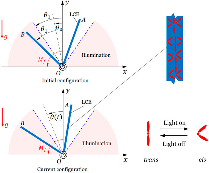
FIGURE 1. Schematic of an inverted pendulum made up of a V-shaped optically responsive LCE bar. Under steady illumination, the inverted pendulum can be self-stabilized due to the reversal of gravity moment resulting from light-driven contraction of the LCE bars.
According to angular momentum theorem, dynamics of the LCE inverted pendulum are governed by
where the angular momentum
where
where
The current lengths of OA and OB bars are
where
where
In Eq. 1,
where the gravity moment
B. Dynamic LCE Model
To determine the motion of the inverted pendulum, we first obtain the current lengths of OA and OB, which depend on the number fraction of cis isomers in the LCE bars. Here, the well-established dynamic LCE model is utilized to determine the number fraction (Warner and Terentjev, (2003)). Generally, the number fraction of cis isomers depends on thermal excitation from trans to cis, thermally driven relaxation from cis to trans, and light-driven trans-to-cis isomerization. Considering that thermal excitation from trans to cis is often negligible relative to the light-driven excitation, the evolution of the number fraction of bent cis isomers is derived as (Warner and Terentjev, (2003)),
where
where
In the dark zone, namely,
By defining the dimensionless quantities
and in the dark zone, Eq. 10 is rewritten as
C. Governing Equations of the LCE Inverted Pendulum
Here, we define the following dimensionless quantities:
Considering that the width is much smaller than the amplitude of oscillation, and the time of the instantaneous transition between bright and dark is also much smaller than a period, the transition time is ignored in the computation. Combining Eqs 2–5, 11, 12 leads to for
where,
,
where,
,
D. Solution Method
Equations 13, 14 are ordinary differential equations with variable coefficients, and there exists no analytic solution. Hereon, the classic fourth order Runge–Kutta method is used to numerically solve the ordinary differential equations by software Matlab. We first transform the second order ordinary differential equation with variable coefficients into two first order ordinary differential equations with variable coefficients. Therefore, the governing equations are rewritten as
where
The classic fourth order Runge–Kutta method is used to solve the problem, The final steady-state of the inverted pendulum is obtained by iteration. When the bar switches between light on and light off, the evolution law is correspondingly converted between Eqs 11, 12. At the conversion moment, the cis number fraction
III. Two Motion Modes and Mechanisms
After numerical computations with respect to Eqs 13, 14 in Sec. IIC, a series of results can be obtained with the variation of physical parameters related to oscillation. In numerical calculations, we choose the typical values of physical parameters from accessible experiments (Marshall and Terentjev, (2013); Nagele et al. (1997)) as follows:
A. Self-Stabilized Oscillation of the LCE Inverted Pendulum
Figure 2 shows two typical motion modes of the LCE inverted pendulum: the unstable static mode and the self-stabilized oscillation mode. Figures 2A,B, respectively, draw the time series curve and its phase diagram of the rotation angle of the typical static mode for
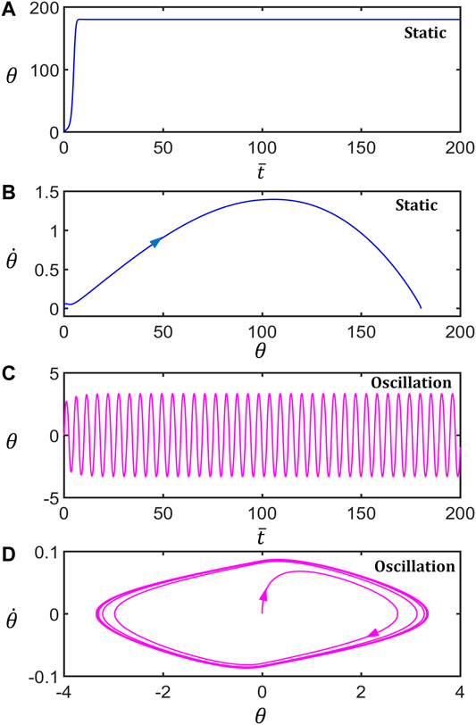
FIGURE 2. Two motion modes of the light-powered inverted pendulum. (A) and (C) are the time series curves of the unstable static mode
B. Mechanisms of the Self-Stabilized Oscillation
To study how the LCE inverted pendulum compensates for the damping dissipation to maintain the periodic oscillation, the time series curves of each physical quantity in a typical mode of the inverted pendulum are given in Figure 3. Parameters are set as follows:
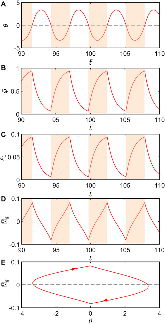
FIGURE 3. Mechanism of the self-stabilized oscillation of the LCE inverted pendulum. Parameters are set:
The inverted pendulum in this paper is stabilized through self-excited oscillation and is much different from the well-known Kapitza’s pendulum stabilized through parametrically excited oscillations (Kapitza (1951)). Generally, parametrically excited oscillations arise from the external excitation of periodic or system parameters and usually adjust the parameters of the oscillatory system through a clear process-independent time law. The control differential equations for parametrically excited oscillations generally have periodic time-varying coefficients. However, compared with parametrically excited oscillations, self-excited oscillations are caused by the internal interaction of the elements within the system in external constant energy situations, and the system can maintain the periodic motion of equal amplitude through process-related self-regulation and feedback control (Ding (2010)).
IV. Parametric Study
Generally, the system oscillates with a limit cycle around a naturally unstable upper position due to the material properties. Considering the theoretical analysis of the bifurcation is very difficult, alternatively, we perform detailed numerical analysis to obtain the critical condition for triggering self-excited oscillation of the pendulum. Furthermore, we also investigate the effects of the system parameters on the amplitude and period of the self-stabilized oscillation of the inverted pendulum through the variable-controlling method.
A. Effect of the Vertex Angle
Figure 4 illustrates the effect of
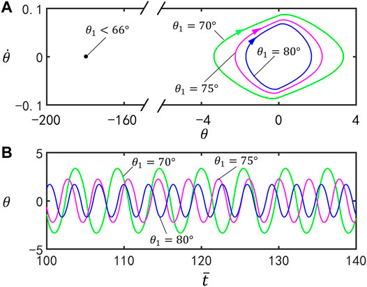
FIGURE 4. Effect of the vertex angle on self-stabilized oscillation of the inverted pendulum for
B. Effect of the Initial Position
Figure 5 delineates the effect of the initial position
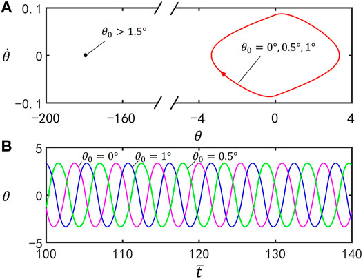
FIGURE 5. Effect of the initial position
C. Effect of the Light Intensity
Figure 6 plots the effect of the dimensionless light intensity
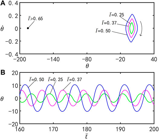
FIGURE 6. Effects of the light intensity
D. Effect of the Contraction Coefficient
Figure 7 reflects the effect of the contraction coefficient
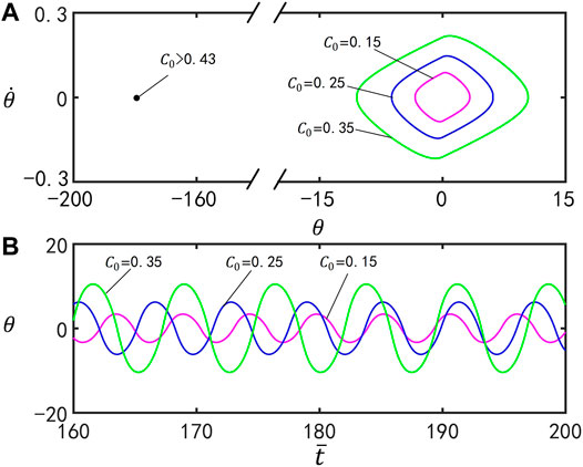
FIGURE 7. Effect of the contraction coefficient
E. Effect of the Damping Coefficient
Figure 8 illustrates the effect of the dimensionless damping coefficient
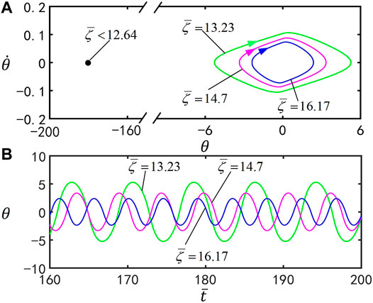
FIGURE 8. Effect of the damping coefficient
F. Effect of the Gravitational Acceleration
Figure 9 plots the effect of the dimensionless gravitational acceleration
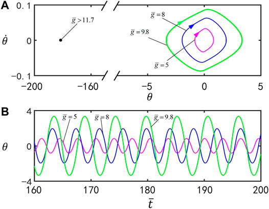
FIGURE 9. Effect of the gravitational acceleration
The above results show that the increase of the light intensity, contraction coefficient, and gravitational acceleration, and the decrease of the vertex angle and damping coefficient are more conducive to the stability of the inverted pendulum system. Detailed numerical calculation shows that the optimal parameter combination is
V. Conclusion
In this paper, self-excited oscillation is adopted to propose a new self-stabilized inverted pendulum, which consists of a V-shaped optically responsive LCE bar. Based on the well-established dynamic LCE model, the nonlinear dynamic theory of the LCE inverted pendulum under steady illumination is formulated, and numerical calculation shows that the inverted pendulum system always evolves into the static state or the self-stabilized oscillation state. The mechanism of the self-stabilized oscillation is elucidated by the reversal of the gravity moment of the inverted pendulum. The amplitude and frequency of the self-oscillation can be designed by modulating several system parameters. The self-stabilized inverted pendulum fueled by steady illumination is sustainable and does not need an additional controller. The results provide new insights into understanding the self-oscillation phenomenon and offer new designs of inverted pendulum systems for potential applications in robotics, military industry, aerospace and, other fields.
Data Availability Statement
The original contributions presented in the study are included in the article/Supplementary Material, further inquiries can be directed to the corresponding author.
Author Contributions
QC conducted theoretical formulation and numerical calculation and wrote the article. LZ helped in the numerical calculations and edited the manuscript. KL developed the concept and edited the article. All authors contributed to article revision, development and approved the submitted version.
Funding
This research was supported by National Natural Science Foundation of China (Grant No. 12172001), University Natural Science Research Project of Anhui Province (Grant No. KJ2020A0449) and Doctoral Startup Foundation from Anhui Jianzhu University (Grant No. 2020QDZ14).
Conflict of Interest
The authors declare that the research was conducted in the absence of any commercial or financial relationships that could be construed as a potential conflict of interest.
The handling Editor declared a past co-authorship with one of the authors (KL).
Publisher’s Note
All claims expressed in this article are solely those of the authors and do not necessarily represent those of their affiliated organizations, or those of the publisher, the editors and the reviewers. Any product that may be evaluated in this article, or claim that may be made by its manufacturer, is not guaranteed or endorsed by the publisher.
References
Balcerzak, M. (2020). Novel Method of Friction Identification with Application for Inverted Pendulum Control System. Mech. Mech. Eng. 22, 1239–1246. doi:10.2478/mme-2018-0095
Bartlett, N. W., Tolley, M. T., Overvelde, J. T. B., Weaver, J. C., Mosadegh, B., Bertoldi, K., et al. (2015). A 3D-Printed, Functionally Graded Soft Robot Powered by Combustion. Science 349, 161–165. doi:10.1126/science.aab0129
Baumann, A., Sánchez-Ferrer, A., Jacomine, L., Martinoty, P., Le Houerou, V., Ziebert, F., et al. (2018). Motorizing Fibres with Geometric Zero-Energy Modes. Nat. Mater 17, 523–527. doi:10.1038/s41563-018-0062-0
Bayram, A., and Kara, F. (2020). Design and Control of Spatial Inverted Pendulum with Two Degrees of freedom. J. Braz. Soc. Mech. Sci. Eng. 42, 501. doi:10.1007/s40430-020-02580-3
Boissonade, J., and Kepper, P. D. (2011). Multiple Types of Spatio-Temporal Oscillations Induced by Differential Diffusion in the Landolt Reaction. Phys. Chem. Chem. Phys. 13, 4132–4137. doi:10.1039/c0cp01653e
Chakrabarti, A., Choi, G. P. T., and Mahadevan, L. (2020). Self-excited Motions of Volatile Drops on Swellable Sheets. Phys. Rev. Lett. 124, 258002. doi:10.1103/PhysRevLett.124.258002
Cheng, Q., Liang, X., and Li, K. (2021). Light-powered Self-Excited Motion of a Liquid crystal Elastomer Rotator. Nonlinear Dyn. 103, 2437–2449. doi:10.1007/s11071-021-06250-4
Cheng, Y. C., Lu, H. C., Lee, X., Zeng, H., and Priimagi, A. (2019). Kirigami‐Based Light‐Induced Shape‐Morphing and Locomotion. Adv. Mater. 32, 1906233. doi:10.1002/adma.201906233
Ding, W. (2010). Self-Excited Vibration: Theory, Paradigms and Research Methods. Berlin Heidelberg: Tsinghua University Press, Beijing and Springer-Verlag. ISBN:9783540697404.
Gelebart, A. H., Jan Mulder, D., Varga, M., Konya, A., Vantomme, G., Meijer, E. W., et al. (2017). Making Waves in a Photoactive Polymer Film. Nature 546, 632–636. doi:10.1038/nature22987
Gonzalez, O., and Rossiter, A. (2020). Fast Hybrid Dual Mode NMPC for a Parallel Double Inverted Pendulum with Experimental Validation. IET Control. Theor. Appl 14, 2329–2338. doi:10.1049/iet-cta.2020.0130
Hauser, A. W., Sundaram, S., and Hayward, R. C. (2018). Photothermocapillary Oscillators. Phys. Rev. Lett. 121, 158001. doi:10.1103/PhysRevLett.121.158001
Hu, W., Lum, G. Z., Mastrangeli, M., and Sitti, M. (2018). Small-scale Soft-Bodied Robot with Multimodal Locomotion. Nature 554, 81–85. doi:10.1038/nature25443
Huang, H., and Aida, T. (2019). Towards Molecular Motors in Unison. Nat. Nanotechnol. 14, 407. doi:10.1038/s41565-019-0414-1
Junkun, M., Coogler, K., and Suh, M. (2020). Inquiry-based Learning: Development of an Introductory Manufacturing Processes Course Based on a mobile Inverted Pendulum Robot. Int. J. Mech. Eng. Educ. 48, 371–390. doi:10.1177/0306419019844257
Kapitza, P. L. (1951). Dynamic Stability of the Pendulum with Vibrating Suspension point (In Russian). Sov. Phys. JETP 21, 588–597.
Kim, H., Sundaram, S., Kang, J.-H., Tanjeem, N., Emrick, T., and Hayward, R. C. (2021). Coupled Oscillation and Spinning of Photothermal Particles in Marangoni Optical Traps. Proc. Natl. Acad. Sci. USA 118 (18), e2024581118. doi:10.1073/pnas.2024581118
Kinoshita, S. (2013). Introduction to Nonequilibrium Phenomena. Elsevier, 1–59. doi:10.1016/B978-0-12-397014-5.00001-8
Kumar, K., Knie, C., Bléger, D., Peletier, M. A., Friedrich, H., Hecht, S., et al. (2016). A Chaotic Self-Oscillating Sunlight-Driven Polymer Actuator. Nat. Commun. 7, 11975. doi:10.1038/ncomms11975
Lahikainen, M., Zeng, H., and Priimagi, A. (2018). Reconfigurable Photoactuator through Synergistic Use of Photochemical and Photothermal Effects. Nat. Commun. 9, 4148. doi:10.1038/s41467-018-06647-7
Lee, K. M., Smith, M. L., Koerner, H., Tabiryan, N., Vaia, R. A., Bunning, T. J., et al. (2011). Photodriven, Flexural-Torsional Oscillation of Glassy Azobenzene Liquid Crystal Polymer Networks. Adv. Funct. Mater. 21, 2913–2918. doi:10.1002/adfm.201100333
Li, K., Wu, P., and Cai, S. (2014). Chemomechanical Oscillations in a Responsive Gel Induced by an Autocatalytic Reaction. J. Appl. Phys. 116, 043523. doi:10.1063/1.4891520
Li, M.-H., Keller, P., Li, B., Wang, X., and Brunet, M. (2003). Light-driven Side-On Nematic Elastomer Actuators. Adv. Mater. 15, 569–572. doi:10.1002/adma.200304552
Maeda, S., Hara, Y., Sakai, T., Yoshida, R., and Hashimoto, S. (2007). Self-walking Gel. Adv. Mater. 19, 3480–3484. doi:10.1002/adma.200700625
Marshall, J. E., and Terentjev, E. M. (2013). Photo-sensitivity of Dye-Doped Liquid crystal Elastomers. Soft Matter 9, 8547–8551. doi:10.1039/C3SM51091C
Nägele, T., Hoche, R., Zinth, W., and Wachtveitl, J. (1997). Femtosecond Photoisomerization of Cis-Azobenzene. Chem. Phys. Lett. 272, 489–495. doi:10.1016/S0009-2614(97)00531-9
Nivedita, B., and Soumitro, B. (2020). Dynamics of a System of Coupled Inverted Pendula with Vertical Forcing. Chaos Soliton. Fract. 141, 110358. doi:10.1016/j.chaos.2020.110358
Nocentini, S., Parmeggiani, C., Martella, D., and Wiersma, D. S. (2018). Optically Driven Soft Micro Robotics. Adv. Opt. Mater. 6, 1800207. doi:10.1002/adom.201800207
Serak, S., Tabiryan, N., Vergara, R., White, T. J., Vaia, R. A., and Bunning, T. J. (2010). Liquid Crystalline Polymer Cantilever Oscillators Fueled by Light. Soft Matter 6, 779–783. doi:10.1039/b916831a
Uchida, E., Azumi, R., and Norikane, Y. (2015). Light-induced Crawling of Crystals on a Glass Surface. Nat. Commun. 6, 7310. doi:10.1038/ncomms8310
Warner, M., and Terentjev, E. M. (2003). Liquid crystal Elastomers. Oxford University Press. ISBN:9780198527671.
Wehner, M., Truby, R. L., Fitzgerald, D. J., Mosadegh, B., Whitesides, G. M., Lewis, J. A., et al. (2016). An Integrated Design and Fabrication Strategy for Entirely Soft, Autonomous Robots. Nature 536, 451–455. doi:10.1038/nature19100
Yakacki, C. M., Saed, M., Nair, D. P., Gong, T., Reed, S. M., and Bowman, C. N. (2015). Tailorable and Programmable Liquid-Crystalline Elastomers Using a Two-Stage Thiol-Acrylate Reaction. RSC Adv. 5, 18997–19001. doi:10.1039/c5ra01039j
Yamada, M., Kondo, M., Mamiya, J.-i., Yu, Y., Kinoshita, M., Barrett, C. J., et al. (2008). Photomobile Polymer Materials: Towards Light-Driven Plastic Motors. Angew. Chem. Int. Ed. 47, 4986–4988. doi:10.1002/anie.200800760
Keywords: inverted pendulum, stabilization, liquid crystal elastomer, optically-responsive, self-sustained motion
Citation: Cheng Q, Zhou L and Li K (2022) A Self-Stabilized Inverted Pendulum Made of Optically Responsive Liquid Crystal Elastomers. Front. Robot. AI 8:808262. doi: 10.3389/frobt.2021.808262
Received: 03 November 2021; Accepted: 24 November 2021;
Published: 11 January 2022.
Edited by:
Qiguang He, University of Pennsylvania, United StatesReviewed by:
Yue Gu, University of California, San Diego, United StatesYue Zheng, University of Southern California, United States
Xudong Liang, Harbin Institute of Technology, Shenzhen, China
Copyright © 2022 Cheng, Zhou and Li. This is an open-access article distributed under the terms of the Creative Commons Attribution License (CC BY). The use, distribution or reproduction in other forums is permitted, provided the original author(s) and the copyright owner(s) are credited and that the original publication in this journal is cited, in accordance with accepted academic practice. No use, distribution or reproduction is permitted which does not comply with these terms.
*Correspondence: Kai Li, a2xpQGFoanp1LmVkdS5jbg==