Sensitivity analysis of compressive sensing solutions

The compressive sensing framework finds a wide range of applications in signal processing, data analysis, and fusion. Within this framework, various methods have been proposed to find a sparse solution x from a linear measurement model y = Ax. In practice, the linear model is often an approximation. One basic issue is the robustness of the solution in the presence of uncertainties. In this paper, we are interested in compressive sensing solutions under a general form of measurement y = (A + B)x + v in which B and v describe modeling and measurement inaccuracies, respectively. We analyze the sensitivity of solutions to infinitesimal modeling error B or measurement inaccuracy v. Exact solutions are obtained. Specifically, the existence of sensitivity is established and the equation governing the sensitivity is obtained. Worst-case sensitivity bounds are derived. The bounds indicate that sensitivity is linear to measurement inaccuracy due to the linearity of the measurement model, and roughly proportional to the solution for modeling error. An approach to sensitivity reduction is subsequently proposed.

1. Introduction

Consider the following minimization problem from perfect measurements

$\min \left|\right|x{\left|\right|}_{l_0},\text{\hspace{0.17em}subject\hspace{0.17em}to\hspace{0.17em}}y=\mathit{Ax},$ (1)

where y ∈ R^m is a vector of measurements, x ∈ Rⁿ is the vector to be solved, A ∈ R^m×n is a matrix, and l₀ denotes the l₀ norm, i.e., the number of non-zero entries. In the compressive sensing framework, the number of measurements available is far smaller than the dimension of the solution x, i.e., m ≪ n. Because the l₀ norm is not convex, equation (1) is a combinatorial optimization problem, solving, which directly is computationally intensive and often prohibitive for problems of practical interest. Therefore, equation (1) is replaced with the following l₁ minimization problem

$\min \left|\right|x{\left|\right|}_{l_1},\text{\hspace{0.17em}subject\hspace{0.17em}to\hspace{0.17em}}y=\mathit{Ax},$ (2)

where the l₁ norm is defined as $\left|\right|x{\left|\right|}_{l_1}={\displaystyle {\sum }_i\left|x_i\right|}$. Note that the matrix A in equations (1) or (2) is assumed to be known exactly and that y is free from measurement inaccuracy. In practice, the problem formulation equation (2) is often an approximation because there may exist modeling errors in A and measurement inaccuracies in y. Therefore, a realistic measurement equation would be

$y=\left[A+B\left(\mathrm{\theta }\right)\right]x+\upsilon \left(\mathrm{\theta }\right),$ (3)

where θ = [θ_j] ∈ R^p is a vector of unknown parameters, B(θ) ∈ R^m×n is a matrix describing modeling errors, and v(θ) ∈ R^m is measurement noise. One appealing feature of the measurement form equation (3) is that it can incorporate prior knowledge of the inaccuracies. For example, we may have

$B\left(\mathrm{\theta }\right)={\displaystyle \sum _j}{\mathrm{\theta }}_j{B}_j,\upsilon \left(\mathrm{\theta }\right)={\displaystyle \sum _j}{\mathrm{\theta }}_j{\upsilon }_j,$ (4)

where B_j and v_j are known matrices or vectors of appropriate dimensions from prior knowledge. When no prior knowledge is available, B_j and v_j can be chosen as the entry indicator matrix or vector, e.g., v_j has 1 for the j-th entry of v(θ) and 0 everywhere else. The form equation (3) can be used to describe a wide range of inaccuracies. In equation (4), θ_j is the unknown magnitude of inaccuracy. Another interpretation of the measurement form equation (3) is that it represents structured uncertainties and can be used to describe the characteristics of inaccuracies for different measurements. For example, in multi-spectrum imaging, the noise characteristics are different for different spectrum. Images taken from different views or at different times may exhibit different noise characteristics. In the setting of a sensor network, a particular sensor may produce bad data due to malfunctioning, which likely leads to different characteristics of inaccuracy compared with other functioning sensors. Without loss of generality, it is assumed that the nominal value of θ is 0, which corresponds to the case with perfect modeling and measurements. Under measurement equation (3), the problem equation (2) can be recast as

$\min \left|\right|x{\left|\right|}_{l_1},\text{\hspace{0.17em}subject\hspace{0.17em}to\hspace{0.17em}}y=\left[A+B\left(\mathrm{\theta }\right)\right]x+\upsilon \left(\mathrm{\theta }\right).$ (5)

A natural question is how sensitive is the solution of equation (5) to small perturbations at θ, without loss of generality, particularly around θ = 0? Because equation (2) is often only an approximation for problems of practical interest, such sensitivity characterizes the robustness of the solution to modeling or measurement inaccuracies. Among the vast literature on compressive sensing, there has been significant interest in analyzing the robustness of compressive sensing solutions in the presence of measurement inaccuracies. One widely adopted approach, such as those in Candes et al. (2006) and Candes (2008), is to reformulate the problem equation (2) as

$\min \left|\right|x{\left|\right|}_{l_1},\text{\hspace{0.17em}subject\hspace{0.17em}to\hspace{0.17em}}\left|\right|y-\mathit{Ax}{\left|\right|}_{l_2}\le \mathrm{ϵ},$ (6)

in which ϵ is a tolerable bound of solution inaccuracy, and the l₂ norm is defined as $\left|\right|x{\left|\right|}_{l_2}={\left({\sum }_i{x}_i^2\right)}^{1∕2}$. Existing literature on equation (6) is extensive. Interested readers are referred to Donoho (2006), Candes and Wakin (2008), and Eldar and Kutyniok (2012) for a comprehensive treatment and literature review. Of particular relevance to this paper, Donoho et al. (2011) (Donoho and Reevew, 2012) analyzed sensitivity of signal recovery solutions to the relaxation of sparsity under the Least Absolute Shrinkage and Selection Operator (LASSO) problem formulation and obtained asymptotic performance bounds in terms of underlying parameters in the methods of finding the solutions. Herman and Strohmer (2010) derived l₂ bounds between the solutions of equations (2) and (5) in terms of perturbation bounds of unknown B(θ) and v(θ). Only the magnitudes (i.e., $\left|\right|.{\left|\right|}_{l_2}$ bounds) of B(θ) and v(θ) are assumed known. Chi et al. (2011) analyzed solution bounds to modeling errors of unknown B(θ) and v(θ). The goal was to investigate the effects of basis mismatch since the matrix A is also known as the basis matrix in compressive sensing. Upper bounds of solution deviation were obtained. The treatments in those papers considered both strictly sparse signals and compressible signals, i.e., the ordered entries of the signal vector decay exponentially fast. The bounds are of the following form Upper bounds of solutions are obtained (Candes et al., 2006; Candes, 2008)

$\left|\right|x\left(\mathrm{\theta }\right)-x{\left|\right|}_{l_2}\le C_1\left|\right|x-x_k{\left|\right|}_{l_1}+C_2\mathrm{ϵ},$

where C₁ and C₂ are constants dependent of A, k is the sparsity of x, and x_k is x with all but the k-largest entries set to zero. Recent publications (Arias-Castro and Eldar, 2011; Davenport et al., 2012; Tang et al., 2013) analyzed the statistical bounds when measurement inaccuracies are modeled as Gaussian noises. A recent publication (Moghadam et al., 2014) after this paper was written-derived sensitivity bounds while this paper seeks exact solutions to sensitivity.

The objective of this paper is to analyze the sensitivity of compressive sensing solutions to perturbations (inaccuracies) in matrix A and measurement y, i.e., the sensitivity of solutions to equation (5) to the unknown parameter θ at θ = 0. Such sensitivity characterizes the effects of infinitesimal perturbations in modeling and measurements. Deterministic problem setting is adopted, and the true solution is assumed to be k-sparse. The sensitivity is local at θ = 0. Exact expressions of the sensitivity are derived. The results of this paper provide complementary insights regarding the effects of modeling and measurement inaccuracies on compressive sensing solutions.

The rest of the paper is arranged as the follows: in Section 2, we examine the continuity of the solution x(θ) at θ = 0. In Section 3, we establish the existence, finiteness, and equation for the sensitivity of x(θ) at θ = 0. Bounds for worst-case infinitesimal perturbations are derived in Section 4. An approach to sensitivity reduction is proposed in Section 5. A numerical example is provided in Section 6 to illustrate the sensitivity reduction algorithms. Finally, concluding remarks are provided in Section 7.

In this paper, we use lower case letters to denote column vectors, upper case letters to denote matrices. For parameterized vectors, the following notational conventions, if exist, will be adopted.

$\begin{array}{ll}\hfill \nabla \upsilon \left(\mathrm{\theta }\right)& =\left[\frac{\mathrm{\partial \upsilon }\left(\mathrm{\theta }\right)}{\partial {\mathrm{\theta }}_1}& \frac{\mathrm{\partial \upsilon }\left(\mathrm{\theta }\right)}{\partial {\mathrm{\theta }}_2}& ...& \frac{\mathrm{\partial \upsilon }\left(\mathrm{\theta }\right)}{\partial {\mathrm{\theta }}_p}\\ \right]\in R^{m\times p},\\ \hfill \nabla \mathit{B}\left(\mathrm{\theta }\right)& =\left[\frac{\mathit{\partial B}\left(\mathrm{\theta }\right)}{\partial {\mathrm{\theta }}_1}& \frac{\mathit{\partial B}\left(\mathrm{\theta }\right)}{\partial {\mathrm{\theta }}_2}& ...& \frac{\mathit{\partial B}\left(\mathrm{\theta }\right)}{\partial {\mathrm{\theta }}_p}\\ \right]\in R^{m\times \mathit{np}}.\end{array}$

Consequently, for a vector x ∈ Rⁿ independent of θ,

$\nabla \left[\mathit{B}\left(\mathrm{\theta }\right)x\right]=\left[\hfill \frac{\mathit{\partial B}\left(\mathrm{\theta }\right)}{\partial {\mathrm{\theta }}_1}x\hfill & \hfill \frac{\mathit{\partial B}\left(\mathrm{\theta }\right)}{\partial {\mathrm{\theta }}_2}x\hfill & \hfill ...\hfill & \hfill \frac{\mathit{\partial B}\left(\mathrm{\theta }\right)}{\partial {\mathrm{\theta }}_p}x\hfill \\ \hfill \hfill \right]\in R^{m\times p}.$

For notational consistence, the l₂ norm of a matrix A = [a_i,j] is defined as the Frobenius norm, $\left|\right|A{\left|\right|}_{l_2}={\left({\sum }_{i,j}{a}_{i,j}^2\right)}^{1∕2}$.

2. Solution Continuity

Let x(θ) denote the solution to equation (5). Without confusion, we reserve x = x(0) to denote a solution to the unperturbed problem equation (2). In this section, we examine the continuity of x(θ) in the neighborhood of θ = 0. A vector x ∈ Rⁿ is said to be k-sparse, k ≪ n, if it has at most k non-zero entries (Candes et al., 2006). In the compressive sensing framework, we are interested in k-sparse solutions.

Without further assumption, the existence of a (sparse) solution to the optimization problem equation (5) is not sufficient in guaranteeing the continuity of x(θ) near θ = 0. To illustrate this issue, consider the following example.

Example 2.1. Consider the problem equation (5) with

$y=1,A=\left[\hfill 1\hfill & \hfill 1+\mathrm{\theta }\hfill \\ \hfill \hfill \right]$

near θ = 0. Then the minimum $\left|\right|x{\left|\right|}_{l_1}$ is achieved by

$x\left(\mathrm{\theta }\right)=\left\{\begin{array}{cc}\left[\begin{array}{c}\hfill 1\hfill \\ \hfill 0\hfill \end{array}\right],\hfill & \text{\hspace{0.17em}if\hspace{0.17em}}\mathrm{\theta }<0\hfill \\ \hfill \\ \mathrm{\alpha }\left[\begin{array}{c}\hfill 1\hfill \\ \hfill 0\hfill \end{array}\right]+\left(1-\mathrm{\alpha }\right)\left[\begin{array}{c}\hfill 0\hfill \\ \hfill 1\hfill \end{array}\right],\text{\hspace{0.17em}for\hspace{0.17em}any\hspace{0.17em}}0\le \mathrm{\alpha }\le 1\hfill & \text{\hspace{0.17em}if\hspace{0.17em}}\mathrm{\theta }=0\hfill \\ \hfill & \hfill \\ \left[\begin{array}{c}\hfill 0\hfill \\ \hfill 1∕\left(1+\mathrm{\theta }\right)\hfill \end{array}\right],\hfill & \text{\hspace{0.17em}if\hspace{0.17em}}\mathrm{\theta }>0.\hfill \end{array}\right.$

It’s clear that the solution x(θ) is not continuous at θ = 0.

In Example 2.1, the solution is not unique at θ = 0. It turns out that the uniqueness of the solution is critical in guaranteeing the continuity of the solution near θ = 0.

One popular approach to finding the solution to equation (5) is to solve the following LASSO problem.

$\underset{x\left(\mathrm{\theta }\right)}{\min }\left\{\frac{1}{2}\left|\right|y-\left[\left(A+\mathit{B}\left(\mathrm{\theta }\right)\right)x\left(\mathrm{\theta }\right)+\upsilon \left(\mathrm{\theta }\right)\right]{\left|\right|}_{l_2}^2+\mathrm{\tau }\left|\right|x\left(\mathrm{\theta }\right){\left|\right|}_{l_1}\right\}$ (7)

which τ > 0 is a weighting parameter.

Theorem 2.1. Assume that both B(θ) and v(θ) are continuous at θ = 0, B(0) = 0, v(0) = 0, AA^T is positive definite, and that the solution x(θ) to equation (7) is unique at θ = 0. Then, x(θ) is continuous at θ = 0, i.e.,

$\underset{\mathrm{\theta }\to 0}{\lim }x\left(\mathrm{\theta }\right)=x,$ (8)

where x is the solution of equation (7) at θ = 0.

Proof. Consider

$\widehat{x}\left(\mathrm{\theta }\right)=\left[A+B\left(\mathrm{\theta }\right)\right]{\left[\left(A+B\left(\mathrm{\theta }\right)\right){\left(A+B\left(\mathrm{\theta }\right)\right)}^T\right]}^{-1}\left(y-\upsilon \left(\mathrm{\theta }\right)\right).$

Then $\widehat{x}(\theta )$ is the Moore–Penrose pseudoinverse solution to $y=[A+B(\theta )]\widehat{x}(\theta )+\upsilon (\theta )$. Under the assumptions that AA^T is positive definite and that both B(θ) and v(θ) are continuous at θ = 0 with B(0) = 0, v(0) = 0, we know that $\widehat{x}(\theta )$ is continuous and uniformly bounded in a small neighborhood of θ = 0, i.e., there exist c > 0, δ > 0 such that $\left|\right|\widehat{x}\left(\mathrm{\theta }\right){\left|\right|}_{l_1}\le c$ for all $\left|\right|\mathrm{\theta }{\left|\right|}_{l_2}\le \mathrm{\delta }$. Because x(θ) is the optimal solution to equation (7) while $\widehat{x}\left(\mathrm{\theta }\right)$ may not, we have

$\begin{array}{l}\mathrm{\tau }\left|\right|x\left(\mathrm{\theta }\right){\left|\right|}_{l_1}\le \frac{1}{2}\left|\right|y-\left[\left(A+B\left(\mathrm{\theta }\right)\right)x\left(\mathrm{\theta }\right)+\upsilon \left(\mathrm{\theta }\right)\right]{\left|\right|}_{l_2}^2+\mathrm{\tau }\left|\right|x\left(\mathrm{\theta }\right){\left|\right|}_{l_1}\hfill \\ \le \frac{1}{2}\left|\right|y-\left[\left(A+B\left(\mathrm{\theta }\right)\right)\widehat{x}\left(\mathrm{\theta }\right)+\upsilon \left(\mathrm{\theta }\right)\right]{\left|\right|}_{l_2}^2+\mathrm{\tau }\left|\right|\widehat{x}\left(\mathrm{\theta }\right){\left|\right|}_{l_1}=\mathrm{\tau }\left|\right|\widehat{x}\left(\mathrm{\theta }\right){\left|\right|}_{l_1}.\hfill \end{array}$

or

$\left|\right|x\left(\mathrm{\theta }\right){\left|\right|}_{l_1}\le \left|\right|\widehat{x}\left(\mathrm{\theta }\right){\left|\right|}_{l_1}\le c$

for all $\left|\right|\mathrm{\theta }{\left|\right|}_{l_2}\le \mathrm{\delta }$. Therefore, x(θ) is uniformly bounded for all $\left|\right|\mathrm{\theta }{\left|\right|}_{l_2}\le \mathrm{\delta }$.

We next prove equation (8) by contradiction. Assume that equation (8) is not true. Because x(θ) is uniformly bound for all $\left|\right|\mathrm{\theta }{\left|\right|}_{l_2}\le \mathrm{\delta }$, there exists a sequence θ_i, i = 1, 2,…, such that

$\underset{i\to \infty }{\lim }{\mathrm{\theta }}_i=0\text{\hspace{0.17em}and\hspace{0.17em}}\underset{i\to \infty }{\lim }x\left({\mathrm{\theta }}_i\right)=\tilde{x}\ne x.$ (9)

Note that x(θ) is the unique solution to equation (7). It must be that

$\begin{array}{l}\hfill \frac{1}{2}\left|\right|y-\left[\left(A+B\left({\mathrm{\theta }}_i\right)\right)x\left({\mathrm{\theta }}_i\right)+\upsilon \left({\mathrm{\theta }}_i\right)\right]{\left|\right|}_{l_2}^2+\mathrm{\tau }\left|\right|x\left({\mathrm{\theta }}_i\right){\left|\right|}_{l_1}\\ <\frac{1}{2}\left|\right|y-\left[\left(A+B\left({\mathrm{\theta }}_i\right)\right)x+\upsilon \left({\mathrm{\theta }}_i\right)\right]{\left|\right|}_{l_2}^2+\mathrm{\tau }\left|\right|x{\left|\right|}_{l_1}.\hfill \end{array}$

By setting i → ∞, also noting the continuity of B(θ) and v(θ) at θ = 0, we obtain

$\frac{1}{2}\left|\right|y-A\tilde{x}{\left|\right|}_{l_2}^2+\mathrm{\tau }\left|\right|\tilde{x}{\left|\right|}_{l_1}\le \frac{1}{2}\left|\right|y-\mathit{Ax}{\left|\right|}_{l_2}^2+\mathrm{\tau }\left|\right|x{\left|\right|}_{l_1}.$

Therefore, we must have $\widehat{x}=x$ because the solution to equation (7) at θ = 0 is unique, which contradicts equation (9). The contradiction establishes equation (8). ■

Note that the number of rows of A is far smaller than the number of columns, m = n. The positive definiteness of AA^T is equivalent to that all measurements y are not redundant, which is technical and mild. Theorem 2.1 states that the solution to equation (7) is continuous if it is unique at θ = 0. Similarly, we can establish the continuity of the solution to equation (5). The proof is similar to that for Theorem 2.1 and omitted to avoid repetitiveness.

Theorem 2.2. Assume that both B(θ) and v(θ) are continuous at θ = 0, B(0) = 0, v(0) = 0, AA^T is positive definite, and that the solution x(θ) to equation (5) is unique at θ = 0. Then x(θ) is continuous at θ = 0, i.e.,

$\underset{\mathrm{\theta }\to 0}{\lim }x\left(\mathrm{\theta }\right)=x.$ (10)

We introduce the following concept, which is a one-sided relaxation of the Restricted Isometry Property (RIP) (Candes et al., 2006).

Definition 2.1. A matrix A ∈ R^m×n is said to be k-sparse positive definite if there exists a constant c > 0 such that

$\left|\right|\mathit{Ax}{\left|\right|}_{l_2}^2\ge c\left|\right|x{\left|\right|}_{l_2}^2$ (11)

for any k-sparse vector x ∈ Rⁿ.

The 2k-sparse positive definiteness is a sufficient condition for guaranteeing the uniqueness of the optimal solution to equation (5) (Candes, 2008).

3. Solution Sensitivity

In this section, we are interested in the gradient information

$\nabla \mathit{x}\left(\mathrm{\theta }\right)=\left[\hfill \frac{\mathit{\partial x}\left(\mathrm{\theta }\right)}{\partial {\mathrm{\theta }}_1}\hfill & \hfill \frac{\mathit{\partial x}\left(\mathrm{\theta }\right)}{\partial {\mathrm{\theta }}_2}\hfill & \hfill ...\hfill & \hfill \frac{\mathit{\partial x}\left(\mathrm{\theta }\right)}{\partial {\mathrm{\theta }}_p}\hfill \\ \hfill \hfill \right]$ (12)

which, if exists, is an n × p matrix in R^n×p.

The next theorem establishes the existence of the gradient equation (12).

Theorem 3.1. Consider problem equation (5). Assume that both B(θ) and v(θ) are differentiable at θ = 0, B(0) = 0, v(0) = 0, and that there exists a δ > 0 such that A is 3k-sparse positive definite for all $\left|\right|\mathrm{\theta }{\left|\right|}_{l_2}\le \mathrm{\delta }$. Then at θ = 0, the gradient ▽x(θ) exists, is finite, and satisfies

$\mathit{AZ}+\mathit{EX}+W=0,$ (13)

where

$\begin{array}{llll}\hfill Z& =\nabla x\left(\mathrm{\theta }\right){|}_{\mathrm{\theta }=0}\in R^{n\times p},E=\nabla B\left(\mathrm{\theta }\right){|}_{\mathrm{\theta }=0}\in R^{m\times \mathit{np}},W=\nabla \upsilon \left(\mathrm{\theta }\right){|}_{\mathrm{\theta }=0}\in R^{m\times p},& \hfill & \\ \hfill X& =\left[\begin{array}{ccccc}x& 0& 0& ...& 0\\ 0& x& 0& ...& 0\\ ...& ...& ...& ...& ...\\ 0& 0& 0& ...& x\end{array}\right]\in R^{\mathit{np}\times p},\end{array}$

and x is the solution to equation (2).

Proof. For the sake of simple notations, we only prove the theorem for scalar θ. The proof can be extended component wisely to the vector case.

We first establish the existence of ▽x(θ). Let h(θ) = θ⁻¹[x(θ) − x] where x(θ) and x are solutions to the optimization problems equations (5) and (2), respectively.

Under the continuity of B(θ), A + B(θ) is 3k-sparse positive definite with a constant $\tilde{c}$ independent of θ in a small neighborhood of θ = 0 if A is. Therefore,

$\begin{array}{l}\hfill \tilde{c}\left|\right|x-x\left(\mathrm{\theta }\right){\left|\right|}_{l_2}^2\le \left|\right|\left[A+B\left(\mathrm{\theta }\right)\right]\left[x-x\left(\mathrm{\theta }\right)\right]{\left|\right|}_{l_2}^2\le \left|\right|B\left(\mathrm{\theta }\right){\left|\right|}_{l_2}^2\left|\right|x{\left|\right|}_{l_2}^2+\left|\right|\upsilon \left(\mathrm{\theta }\right){\left|\right|}_{l_2}^2.\end{array}$ (14)

or

$\left|\right|h\left(\mathrm{\theta }\right){\left|\right|}_{l_2}^2\le {\tilde{c}}^{-1}\left[\left|\right|{\mathrm{\theta }}^{-1}B\left(\mathrm{\theta }\right){\left|\right|}_{l_2}^2\left|\right|x{\left|\right|}_{l_2}^2+\left|\right|{\mathrm{\theta }}^{-1}\upsilon \left(\mathrm{\theta }\right){\left|\right|}_{l_2}^2\right].$

By assumption, B(θ) and v(θ) are differentiable at θ = 0. The previous inequality shows that h(θ) is uniformly bounded in a small neighborhood of θ = 0. Consequently, there exists a sequence θ⁽ⁱ⁾ → 0 such that

$\widehat{h}\stackrel{▵}{=}\underset{i\to \infty }{\lim }h\left({\mathrm{\theta }}^{\left(i\right)}\right)$ (15)

exists and is finite. Recall that

$\left[A+B\left(\mathrm{\theta }\right)\right]h\left(\mathrm{\theta }\right)=-{\mathrm{\theta }}^{-1}B\left(\mathrm{\theta }\right)x-{\mathrm{\theta }}^{-1}\upsilon \left(\mathrm{\theta }\right)$

and

$\left[A+B\left({\mathrm{\theta }}^{\left(i\right)}\right)\right]h\left({\mathrm{\theta }}^{\left(i\right)}\right)=-{\left({\mathrm{\theta }}^{\left(i\right)}\right)}^{-1}B\left({\mathrm{\theta }}^{\left(i\right)}\right)x-{\left({\mathrm{\theta }}^{\left(i\right)}\right)}^{-1}\upsilon \left({\mathrm{\theta }}^{\left(i\right)}\right).$

Their difference gives

$\begin{array}{l}A\left[h\left(\mathrm{\theta }\right)-h\left({\mathrm{\theta }}^{\left(i\right)}\right)\right]=-B\left(\mathrm{\theta }\right)h\left(\mathrm{\theta }\right)+B\left({\mathrm{\theta }}^{\left(i\right)}\right)h\left({\mathrm{\theta }}^{\left(i\right)}\right)-{\mathrm{\theta }}^{-1}B\left(\mathrm{\theta }\right)x+{\left({\mathrm{\theta }}^{\left(i\right)}\right)}^{-1}B\left({\mathrm{\theta }}^{\left(i\right)}\right)x\hfill \\ -{\mathrm{\theta }}^{-1}\upsilon \left(\mathrm{\theta }\right)+{\left({\mathrm{\theta }}^{\left(i\right)}\right)}^{-1}\upsilon \left({\mathrm{\theta }}^{\left(i\right)}\right)\hfill & & \hfill \end{array}$

or

$\begin{array}{l}\left|\right|A\left[h\left(\mathrm{\theta }\right)-h\left({\mathrm{\theta }}^{\left(i\right)}\right)\right]{\left|\right|}_{l_2}^2\le \left|\right|B\left(\mathrm{\theta }\right)h\left(\mathrm{\theta }\right){\left|\right|}_{l_2}^2+\left|\right|B\left({\mathrm{\theta }}^{\left(i\right)}\right)h\left({\mathrm{\theta }}^{\left(i\right)}\right){\left|\right|}_{l_2}^2\hfill \\ +\left|\right|\left[{\mathrm{\theta }}^{-1}B\left(\mathrm{\theta }\right)-{\left({\mathrm{\theta }}^{\left(i\right)}\right)}^{-1}B\left({\mathrm{\theta }}^{\left(i\right)}\right)\right]x{\left|\right|}_{l_2}^2+\left|\right|{\mathrm{\theta }}^{-1}\upsilon \left(\mathrm{\theta }\right)-{\left({\mathrm{\theta }}^{\left(i\right)}\right)}^{-1}\upsilon \left({\mathrm{\theta }}^{\left(i\right)}\right){\left|\right|}_{l_2}^2.\hfill & & \hfill \end{array}$

Since A is 3k-sparse positive definite, there exists a constant c > 0 such that

$c\left|\right|h\left(\mathrm{\theta }\right)-h\left({\mathrm{\theta }}^{\left(i\right)}\right){\left|\right|}_{l_2}^2\le \left|\right|A\left[h\left(\mathrm{\theta }\right)-h\left({\mathrm{\theta }}^{\left(i\right)}\right)\right]{\left|\right|}_{l_2}^2.$

Consequently,

$\begin{array}{l}c\left|\right|h\left(\mathrm{\theta }\right)-h\left({\mathrm{\theta }}^{\left(i\right)}\right){\left|\right|}_{l_2}^2\le \left|\right|B\left(\mathrm{\theta }\right)h\left(\mathrm{\theta }\right){\left|\right|}_{l_2}^2+\left|\right|B\left({\mathrm{\theta }}^{\left(i\right)}\right)h\left({\mathrm{\theta }}^{\left(i\right)}\right){\left|\right|}_{l_2}^2\hfill \\ +\left|\right|{\mathrm{\theta }}^{-1}B\left(\mathrm{\theta }\right)-{\left({\mathrm{\theta }}^{\left(i\right)}\right)}^{-1}B\left({\mathrm{\theta }}^{\left(i\right)}\right){\left|\right|}_{l_2}^2\left|\right|x{\left|\right|}_{l_1}^2+\left|\right|{\mathrm{\theta }}^{-1}\upsilon \left(\mathrm{\theta }\right)-{\left({\mathrm{\theta }}^{\left(i\right)}\right)}^{-1}\upsilon \left({\mathrm{\theta }}^{\left(i\right)}\right){\left|\right|}_{l_2}^2.\hfill \end{array}$ (16)

The right hand side of equation (16) goes to zero as θ → 0, i → ∞. Therefore,

$\underset{\mathrm{\theta }\to 0,i\to \infty }{\lim }\left|\right|h\left(\mathrm{\theta }\right)-h\left({\mathrm{\theta }}^{\left(i\right)}\right){\left|\right|}_{l_2}^2=0.$

Or equivalently,

$\underset{\mathrm{\theta }\to 0}{\lim }h\left(\mathrm{\theta }\right)=\underset{i\to \infty }{\lim }h\left({\mathrm{\theta }}^{\left(i\right)}\right)=\widehat{h},$ (17)

which establishes that ▽x(θ) exists at θ = 0 and is finite.

Finally, the fact that x(θ) and x are the solutions to problems equations (5) and (2), respectively, gives

$\left[A+B\left(\mathrm{\theta }\right)\right]h\left(\mathrm{\theta }\right)+{\mathrm{\theta }}^{-1}B\left(\mathrm{\theta }\right)x+{\mathrm{\theta }}^{-1}\upsilon \left(\mathrm{\theta }\right)=0.$

Denote $Z\stackrel{▵}{=}\widehat{h}={\lim }_{\mathrm{\theta }\to 0}h\left(\mathrm{\theta }\right)$ which exists and is finite. By setting θ → 0 in the above equation, we obtain

$\mathit{AZ}+\mathit{EX}+W=0$

which is equation (13). This completes the proof of the theorem. ■

Since the solution x(θ) is k-sparse for all θ in a small neighborhood of θ = 0, by focusing on the non-zero entries of x and x(θ), the proof of Theorem 3.1 also shows that each column of Z is k-sparse. The support of Z is the same as that of x.

Equation (13) indicates that only those perturbations in E that corresponds to non-zero entries of x contribute to the sensitivity.

A note is needed regarding the requirement of the 3k-sparse positive definiteness in Theorem 3.1. It has been known in the literature [e.g., Candes (2008) in the form of the Restricted Isometry Property] that 2k-sparse positive definiteness is needed for guaranteeing the uniqueness of a k-sparse solution. The 3k-sparse positive definiteness is needed for ensuring the differentiability of the solution, a higher order property. This is a sufficient condition, and its relaxation is a subject of current effort.

4. Sensitivity Analysis

Equation (13) gives an explicit expression of the sensitivity ▽x(θ) at θ = 0. Theorem 3.1 shows that the k-sparse solution Z is unique for given x, E, and W. In this section, we consider the worst-case perturbations, i.e., the value(s) of E and W that maximizes $\left|\right|Z{\left|\right|}_{l_2}$. It’s obvious that the sensitivity increases when either $\left|\right|E{\left|\right|}_{l_2}$ or $\left|\right|W{\left|\right|}_{l_2}$ increases. We analyze the sensitivity based on normalized perturbations. Specifically, we consider the following

$\begin{array}{llll}\hfill & \underset{E:\left|\right|E{\left|\right|}_{l_2}=1;W=0}{\max }\left|\right|Z{\left|\right|}_{l_2},\underset{E=0;W:\left|\right|W{\left|\right|}_{l_2}=1}{\max }\left|\right|Z{\left|\right|}_{l_2},\text{\hspace{0.17em}and\hspace{0.17em}}\underset{E,W:\left|\right|\left[EW\right]{\left|\right|}_{l_2}=1}{\max }\left|\right|Z{\left|\right|}_{l_2}.& \hfill & \end{array}$

Lemma 4.1. The sensitivity Z satisfies the following relationship

$\begin{array}{ll}\hfill & \underset{E:\left|\right|E{\left|\right|}_{l_2}=1;W=0}{\max }\left|\right|\mathit{AZ}{\left|\right|}_{l_2}=\left|\right|x{\left|\right|}_{l_2},\end{array}$ (18)

$\begin{array}{ll}\hfill & \underset{E=0;W:\left|\right|W{\left|\right|}_{l_2}=1}{\max }\left|\right|\mathit{AZ}{\left|\right|}_{l_2}=1,\end{array}$ (19)

$\begin{array}{ll}\hfill & \underset{E,W:\left|\right|\left[EW\right]{\left|\right|}_{l_2}=1}{\max }\left|\right|\mathit{AZ}{\left|\right|}_{l_2}={(\left|\right|x{\left|\right|}_{l_2}^2+1)}^{1∕2}.\end{array}$ (20)

Proof. According to equation (13), Z satisfies

$\mathit{AZ}=-\mathit{EX}-W.$

Next we consider each of the three cases.

Case I: W = 0. In this case,

$\left|\right|\mathit{AZ}{\left|\right|}_{l_2}=\left|\right|\mathit{EX}{\left|\right|}_{l_2}.$

Recall that

$\mathit{EX}=\left[E_{1}x{E}_{2}x...E_{p}x\right].$

By applying the Cauchy-Schwarz inequality $\left|\right|\mathit{Ax}{\left|\right|}_{l_2}\le \left|\right|A{\left|\right|}_{l_2}\left|\right|x{\left|\right|}_{l_2},$ we obtain

$\begin{array}{lll}\hfill \left|\right|\mathit{EX}{\left|\right|}_{l_2}^2={\displaystyle \sum _{j=1}^p}\left|\right|E_{j}x{\left|\right|}_{l_2}^2\le {\displaystyle \sum _{j=1}^p}\left|\right|E_j{\left|\right|}_{l_2}^2\left|\right|x{\left|\right|}_{l_2}^2=\left({\displaystyle \sum _{j=1}^p}\left|\right|E_j{\left|\right|}_{l_2}^2\right)\left|\right|x{\left|\right|}_{l_2}^2=\left|\right|E{\left|\right|}_{l_2}^2\left|\right|x{\left|\right|}_{l_2}^2.& & \hfill \end{array}$

Therefore,

$\begin{array}{l}\hfill \underset{E:\left|\right|E{\left|\right|}_{l_2}=1;W=0}{\text{sup}}\left|\right|\mathit{AZ}{\left|\right|}_{l_2}=\underset{E:\left|\right|E{\left|\right|}_{l_2}=1;W=0}{\text{sup}}\left|\right|\mathit{EX}{\left|\right|}_{l_2}\le \underset{E:\left|\right|E{\left|\right|}_{l_2}=1}{\max }\left|\right|E{\left|\right|}_{l_2}\left|\right|x{\left|\right|}_{l_2}=\left|\right|x{\left|\right|}_{l_2}.\end{array}$ (21)

Next, we prove that the upper bound is achievable for a specifically chosen E. Let

$\begin{array}{llll}\hfill \widehat{E}& =\left[{\widehat{E}}_1{\widehat{E}}_2...{\widehat{E}}_p\right],{\widehat{E}}_j=\mathrm{\alpha }{e}_m{x}^T,\mathrm{\alpha }={\left(\mathit{mp}\right)}^{-1∕2}\left|\right|x{\left|\right|}_{l_2}^{-1},& \hfill & \\ \hfill e_m& ={\left[11...1\right]}^T\in R^m.& \hfill & \end{array}$

Then

$\left|\right|{\widehat{E}}_j{\left|\right|}_{l_2}^2=\text{trace}\left({\widehat{E}}_j{\widehat{E}}_j^T\right)={\mathrm{\alpha }}^2\left|\right|x{\left|\right|}_{l_2}^2\text{trace}\left(e_m{e}_m^T\right)=m{\mathrm{\alpha }}^2\left|\right|x{\left|\right|}_{l_2}^2$

and

$\left|\right|\widehat{E}{\left|\right|}_{l_2}^2={\displaystyle \sum _{j=1}^p}\left|\right|E_j{\left|\right|}_{l_2}^2={\displaystyle \sum _{j=1}^p}m{\mathrm{\alpha }}^2\left|\right|x{\left|\right|}_{l_2}^2={\mathrm{\alpha }}^2\left(\mathit{mp}\left|\right|x{\left|\right|}_{l_2}^2\right)=1.$

For this $E=\widehat{E}$, we have

$\begin{array}{lll}\hfill \left|\right|\widehat{E}X{\left|\right|}_{l_2}^2={\displaystyle \sum _{j=1}^p}\left|\right|{\widehat{E}}_{j}x{\left|\right|}_{l_2}^2={\displaystyle \sum _{j=1}^p}\left|\right|\mathrm{\alpha }{e}_m{x}^{T}x{\left|\right|}_{l_2}^2={\mathrm{\alpha }}^2\left|\right|x{\left|\right|}_{l_2}^4\mathit{mp}=\left|\right|x{\left|\right|}_{l_2}^2,& & \hfill \end{array}$

or equivalently

$\left|\right|\mathit{AZ}{\left|\right|}_{l_2}=|\widehat{E}X{\left|\right|}_{l_2}=\left|\right|x{\left|\right|}_{l_2}.$ (22)

The combination of equations (21) and (22) gives (18).

Case II: E = 0. In case,

$\left|\right|\mathit{AZ}{\left|\right|}_{l_2}=\left|\right|W{\left|\right|}_{l_2}.$

from which equation (19) follows.

Case III: In general,

$\left|\right|\mathit{AZ}{\left|\right|}_{l_2}=\left|\right|\mathit{EX}+W{\left|\right|}_{l_2}=\left|\right|\tilde{E}\tilde{X}{\left|\right|}_{l_2}$

where

$\begin{array}{lllll}\hfill \tilde{E}& =\left[{\tilde{E}}_1\tilde{x}{\tilde{E}}_2\tilde{x}...{\tilde{E}}_p\tilde{x}\right],\tilde{x}=\left[\begin{array}{c}x\\ 1\end{array}\right],{\tilde{E}}_j& =\left[E_j{W}_j\right],j=1,2,...,p& \hfill & \end{array}$

and W_j is the j-th column of W. By following the proof of Case I, we know that

$\begin{array}{lll}\hfill \underset{E,W:\left|\right|\left[EW\right]{\left|\right|}_{l_2}=1}{\max }\left|\right|\mathit{AZ}{\left|\right|}_{l_2}=\underset{\tilde{E}:\left|\right|\tilde{E}{\left|\right|}_{l_2}=1}{\max }\left|\right|\tilde{E}\tilde{X}{\left|\right|}_{l_2}=\left|\right|\tilde{x}{\left|\right|}_{l_2}={\left(\left|\right|x{\left|\right|}_{l_2}^2+1\right)}^{1∕2}& & \hfill \end{array}$

which establishes equation (20). ■

Equations (18)–(20) show that the worst-case $\left|\right|\mathit{AZ}{\left|\right|}_{l_2}$ is a constant for measurement noise but proportional to the solution vector for modeling error E.

Theorem 4.1. Under the assumptions in Theorem 3.1, the sensitivity Z satisfies the following bounds

$\begin{array}{ll}\hfill & \underset{E:\left|\right|E{\left|\right|}_{l_2}=1;W=0}{\max }\left|\right|Z{\left|\right|}_{l_2}\le {\mathrm{\sigma }}_{\min }^{-1}\left(A\right)\left|\right|x{\left|\right|}_{l_2},\end{array}$ (23)

$\begin{array}{ll}\hfill & \underset{E=0;:\left|\right|W{\left|\right|}_{l_2}=1}{\max }\left|\right|Z{\left|\right|}_{l_2}\le {\mathrm{\sigma }}_{\min }^{-1}\left(A\right),\end{array}$ (24)

$\begin{array}{ll}\hfill & \underset{E:\left|\right|E{\left|\right|}_{l_2}=1;W:\left|\right|W{\left|\right|}_{l_2}=1}{\max }\left|\right|Z{\left|\right|}_{l_2}\le {\mathrm{\sigma }}_{\min }^{-1}\left(A\right){\left(\left|\right|x{\left|\right|}_{l_2}^2+1\right)}^{1∕2}.\end{array}$ (25)

in which σ_min(A) > 0 is the minimal singular value of A.

Proof. Without loss of generality, assume θ is a scalar. Let S be the collection of indices of possibly non-zero entries of Z, Z_S ∈ R^|S| be the vector of non-zero entries of Z corresponding to the indices in S, and A_S be the matrix consisting of corresponding columns of A. Then, A_S is of full column rank if it is k-sparse positive definite, σ_min(A_S) ≥ σ_min(A), and

$\mathit{AZ}=A_S{Z}_S.$

Consider the matrix AZ,

$\begin{array}{l}\hfill \left|\right|\mathit{AZ}{\left|\right|}_{l_2}^2=\text{trace}\left(Z^T{A}^T\mathit{AZ}\right)=\text{trace}\left(Z_S^T{A}_S^T{A}_S{Z}_S\right)\ge \text{trace}\left(Z_S^T{\left({\mathrm{\sigma }}_{\min }\left(A_S\right)\right)}^2{Z}_S\right)\\ \ge {\left({\mathrm{\sigma }}_{\min }\left(A\right)\right)}^2\left|\right|Z_S{\left|\right|}_{l_2}^2={\left({\mathrm{\sigma }}_{\min }\left(A\right)\right)}^2\left|\right|Z{\left|\right|}_{l_2}^2,\hfill & & \hfill \end{array}$

which gives

$\left|\right|Z{\left|\right|}_{l_2}\le {\mathrm{\sigma }}_{\min }^{-1}\left(A\right)\left|\right|\mathit{AZ}{\left|\right|}_{l_2}.$ (26)

The rest follows from combining the previous inequality with equations (18)–(20) in Lemma 4.1. ■

If σ_min(A) is achieved over k columns of A that correspond to the k-sparse signal to be recovered, then the equality in equation (26) holds and the bounds in Theorem 4.1 could be tight. The bounds are not tight in general because the k columns of A corresponding to the indices in S are unknown a priori.

5. Sensitivity Reduction

One natural way of reducing the sensitivity of compressive sensing solutions is to carefully select the basis matrix A so that Z is as small as possible. There has been extensive research on how to select A (Donoho et al., 2006). The general idea is to improve the incoherence of the matrix A, for example, by making A as close as possible to the identity matrix in terms of the RIP property. The problem could be difficult because selecting the correct columns of A from available choices is a combinatorial optimization problem. In this section, we consider an alternative. We assume that the matrix A is given. The objective is to find a solution x that is least sensitive to perturbations B and v. One example where this problem arises is in pattern recognition where each column of A represents a vector in a feature space. The issue is how to classify the pattern based on features of the training data so that the solution is robust to potential perturbations (i.e., noise in data).

We consider to improve the robustness of a signal recovery solution by reducing its sensitivity to model error and measurement inaccuracy. Toward that goal, we reformulate the l₁ optimization problem equation (5) by including a term to penalize high sensitivity. This approach offers an alternative to the conventional approach of basis matrix selection and could be performed after the matrix A is selected.

Solution robustness can be improved by reducing the magnitude of sensitivity. The l_∞ norm is a natural choice because it characterizes the largest entry of a vector or a matrix. Therefore, we consider the following optimization problem.

$\min \left|\right|x{\left|\right|}_{l_1}+\mathrm{\lambda }\left|\right|Z{\left|\right|}_{l_{\infty }},\text{\hspace{0.17em}subject to\hspace{0.17em}}y=\mathit{Ax},\mathit{AZ}+\mathit{EX}+W=0,$ (27)

where λ > 0 is a penalizing weight and the l_∞ norm is defined as $\left|\right|Z{\left|\right|}_{l_{\infty }}={\max }_{i,j}\left|z_{ij}\right|$. Note that Z ∈ R^n×p is a matrix. We convert Z into a vector by defining

$\tilde{z}=\left[\begin{array}{c}\hfill z_1\hfill \\ \hfill z_2\hfill \\ \hfill ⋮\hfill \\ \hfill z_p\hfill \end{array}\right]\in R^{\mathit{np}},$

where for each j, 1 ≤ j ≤ p, z_j is the j-th column of Z. Then problem equation (27) can be re-written as

$\min \left|\right|x{\left|\right|}_{l_1}+\mathrm{\lambda }\left|\right|\tilde{z}{\left|\right|}_{l_{\infty }},\text{\hspace{0.17em}subject to\hspace{0.17em}}\mathit{Cx}+D\tilde{z}=f,$ (28)

in which

$\begin{array}{llll}\hfill C& =\left[\begin{array}{c}A\\ E_1\\ E_2\\ ⋮\\ E_p\end{array}\right]\in R^{\left(m+1\right)p\times n},D=\left[\begin{array}{cccc}0& 0& ...& 0\\ A& 0& ...& 0\\ 0& A& ...& 0\\ ...& ...& ...& ...\\ 0& 0& ...& A\end{array}\right]\in R^{\left(m+1\right)p\times \mathit{np}},& \hfill & \\ \hfill f& =\left[\begin{array}{c}y\\ -w_1\\ -w_2\\ ⋮\\ -w_p\end{array}\right]\in R^{\left(m+1\right)p},\end{array}$

and w_j is the j-th column of W, 1 ≤ j ≤ p.

Several methods are available to solve the optimization problem equation (28), one of which is the Alternating Direction Method of Multipliers (ADMM) (Boyd et al., 2011). In fact, equation (28) is in the standard form of the ADMM problem formulation. There is a trade-off in selecting the method or algorithm to solve the optimization problem equation (28) in terms of accuracy, efficiency, and reliability. We adopt the gradient projection algorithms proposed by Figueiredo et al. (2007) for solving LASSO problems. Toward that end, we consider two modifications: The first modification is to replace the l_∞ norm with the l_v norm defined as $\left|\right|Z{\left|\right|}_{l_{\mathrm{\nu }}}={\left({\displaystyle {\sum }_{i,j}|z_j(i){|}^{\nu }}\right)}^{1/\nu }$ where z_j(i) is the ith entry of z_j-the jth column of Z. It is known that ${\lim }_{\mathrm{\nu }\to \infty }\left|\right|Z{\left|\right|}_{l_{\mathrm{\nu }}}=\left|\right|Z{\left|\right|}_{l_{\infty }}$. So a large v is chosen. To ensure the smoothness of the objective function, v is chosen as an even number. The second modification is to reformulate equation (28) as a modified LASSO problem so that the efficient gradient projection algorithms are applicable with minimum modifications. Finally, it is noted that for each j, z_j(i) = 0 for all i not in the support of x. Consequently, we consider the following optimization problem for sensitivity reduction.

$\begin{array}{l}\hfill \min \mathrm{\tau }\left|\right|x{\left|\right|}_{l_1}+\mathrm{\lambda }\left|\right|\tilde{z}{\left|\right|}_{l_{\mathrm{\nu }}}+\frac{1}{2}\left|\right|\mathit{Cx}+D\tilde{z}-f\left|\right|{}_{l_2}^2\\ \text{subject to\hspace{0.17em}}S\left(x\right)=S\left(z_j\right),j=1,2,...,p\hfill \end{array}$ (29)

where v > 1 is a large even number, τ > 0 and λ > 0 are user-selected weights, S(x) is the set of indices corresponding to possibly non-zero entries of a sparse vector x, i.e., the support of x.

We next provide the algorithmic details of implementing the gradient projection method. First, the problem equation (29) is equivalent to the following constrained optimization problem (Figueiredo et al., 2007).

$\begin{array}{l}\hfill \min F\left(u,r,\tilde{z}\right)\stackrel{▵}{=}\frac{\mathrm{\tau }}{2}{e}^T\left(u+r\right)+\mathrm{\lambda }\left|\right|\tilde{z}{\left|\right|}_{l_{\mathrm{\nu }}}+\frac{1}{2}\left|\right|C\left(r-u\right)+D\tilde{z}-f\left|\right|{}_{l_2}^2\\ \text{subject\hspace{0.17em}to\hspace{0.17em}}u\ge 0,r\ge 0,S\left(r-u\right)=S\left(z_j\right),j=1,2,...,p\hfill \end{array}$ (30)

in which e is the vector of all ones, u = [u_j] ≥ 0 (or r = [r_j] ≥ 0) denotes u_j ≥ 0 (or r_j ≥ 0, respectively) for all j = 1, 2,…, n. The sparse solution x is given by

$x=\frac{1}{2}\left(r-u\right),$

and thus S(r − u) = S(x) in equation (30). The gradient of the objective function $F(u,r,\tilde{z})$ in equation (30) is

$\nabla F\left(u,r,\tilde{z}\right)=\left[\begin{array}{c}\hfill {\nabla }_{u}F\left(u,r,\tilde{z}\right)\hfill \\ \hfill {\nabla }_{r}F\left(u,r,\tilde{z}\right)\hfill \\ \hfill {\nabla }_{\tilde{z}}F\left(u,r,\tilde{z}\right)\hfill \end{array}\right],$ (31)

where

$\begin{array}{llll}\hfill & {\nabla }_{u}F\left(u,r,\tilde{z}\right)=\frac{\mathrm{\tau }}{2}e-\frac{1}{2}{C}^T\left[C\left(r-u\right)+D\tilde{z}-f\right],& \hfill & \\ \hfill & {\nabla }_{r}F\left(u,r,\tilde{z}\right)=\frac{\mathrm{\tau }}{2}e+\frac{1}{2}{C}^T\left[C\left(r-u\right)+D\tilde{z}-f\right],& \hfill & \\ \hfill & {\nabla }_{\tilde{z}}F\left(u,r,\tilde{z}\right)=\mathrm{\lambda }\left|\right|\tilde{z}{\left|\right|}_{l_{\mathrm{\nu }}}^{1-\mathrm{\nu }}{\tilde{z}}^{\mathrm{\nu }-1}+D^T\left[\frac{1}{2}C\left(r-u\right)+D\tilde{z}-f\right],& \hfill & \end{array}$

in which ${\tilde{z}}^{\mathrm{\nu }-1}=\left[{\tilde{z}}_j^{\mathrm{\nu }-1}\right]$ for $\tilde{z}=\left[{\tilde{z}}_j\right]$.

The gradient projection algorithms proposed in Figueiredo et al. (2007) find the optimal solutions iteratively. Let $u^{\left(i\right)},r^{\left(i\right)},{\tilde{z}}^{\left(i\right)}$ denote the values of $u,r,\tilde{z}$ at the ith iteration. Then, at the (i + 1)th iteration, $u^{\left(i+1\right)},r^{\left(i+1\right)},{\tilde{z}}^{\left(i+1\right)}$ are updated according to

$\left[\begin{array}{c}\hfill u^{\left(i+1\right)}\hfill \\ \hfill r^{\left(i+1\right)}\hfill \\ \hfill {\tilde{z}}^{\left(i+1\right)}\hfill \end{array}\right]=\left[\begin{array}{c}\hfill u^{\left(i\right)}+{\mathrm{\eta }}^{\left(i\right)}\left(u^{\left(i+1:i\right)}-u^{\left(i\right)}\right)\hfill \\ \hfill r^{\left(i\right)}+{\mathrm{\eta }}^{\left(i\right)}\left(r^{\left(i+1:i\right)}-r^{\left(i\right)}\right)\hfill \\ \hfill {\tilde{z}}^{\left(i\right)}+{\mathrm{\eta }}^{\left(i\right)}\left({\tilde{z}}^{\left(i+1:i\right)}-{\tilde{z}}^{\left(i\right)}\right)\hfill \end{array}\right]$ (32)

where η⁽ⁱ⁾ ∈ [0,1] is a weighting factor, and the transition values $u^{\left(i+1:i\right)},r^{\left(i+1:i\right)},{\tilde{z}}^{\left(i+1:i\right)}$ are gradient projection updates

$\begin{array}{ll}\hfill u^{\left(i+1:i\right)}& ={\mathrm{\Pi }}_{C^{+}}\left(u^{\left(i\right)}-{\mathrm{\alpha }}^{\left(i\right)}{\nabla }_{u}F\left(u^{\left(i\right)},r^{\left(i\right)},{\tilde{z}}^{\left(i\right)}\right)\right).\end{array}$ (33)

$\begin{array}{ll}\hfill r^{\left(i+1:i\right)}& ={\mathrm{\Pi }}_{C^{+}}\left(r^{\left(i\right)}-{\mathrm{\alpha }}^{\left(i\right)}{\nabla }_{r}F\left(u^{\left(i\right)},r^{\left(i\right)},{\tilde{z}}^{\left(i\right)}\right)\right).\end{array}$ (34)

$\begin{array}{ll}\hfill {\tilde{z}}^{\left(i+1:i\right)}& ={\mathrm{\Pi }}_{S\left(r^{\left(i+1\right)}-u^{\left(i+1\right)}\right)}\left({\tilde{z}}^{\left(i\right)}-{\mathrm{\alpha }}^{\left(i\right)}{\nabla }_{\tilde{z}}F\left(u^{\left(i\right)},r^{\left(i\right)},{\tilde{z}}^{\left(i\right)}\right)\right).\end{array}$ (35)

In equations (33)–(35), α⁽ⁱ⁾ > 0 is the step-size of the gradient algorithm, C⁺ = {u = [u_j] ∈ Rⁿ|u_j ≥ 0,j = 1,2,…n} is the non-negative subspace, S(x) is the support of x as defined in equation (29), and Π_C(u) is the projection operator that projects u onto the subspace C. Because x = 1/2(r − u), the subspace S[r⁽ⁱ⁺¹⁾ − u⁽ⁱ⁺¹⁾] in equation (35) is the subspace of x at the (i + 1)th iteration. To increase the efficiency of the algorithm, the step-size α⁽ⁱ⁾ is selected according to the Armijo rule, i.e., ${\mathrm{\alpha }}^{\left(i\right)}={\mathrm{\alpha }}_0{\mathrm{\beta }}^{i_0}$ in which α₀ is the initial step-size, β ∈ (0,1), and i₀ is the first number in the sequence of α₀, αβ, αβ², αβ³, … that achieves

$\begin{array}{lll}\hfill \underset{i}{\min }F\left({\mathrm{\Pi }}_{C^{+}}\left(u^{\left(i\right)}-{\mathrm{\alpha }}_0{\mathrm{\beta }}^i{\nabla }_{u}F\right),{\mathrm{\Pi }}_{C^{+}}\left(r^{\left(i\right)}-{\mathrm{\alpha }}_0{\mathrm{\beta }}^i{\nabla }_{r}F\right),{\mathrm{\Pi }}_{S\left(r^{\left(i+1\right)}-u^{\left(i+1\right)}\right)}\left({\tilde{z}}^{\left(i\right)}-{\mathrm{\alpha }}_0{\mathrm{\beta }}^i{\nabla }_{\tilde{z}}F\right)\right),& & \hfill \end{array}$

in which the values of ▽F are evaluated at $\left(u^{\left(i\right)},r^{\left(i\right)},{\tilde{z}}^{\left(i\right)}\right)$. Note that the projection of $\tilde{z}$ onto the support of x in equation (35) is unique to solving the optimization problem equation (30).

The value of x at the ith iteration is given by $\frac{1}{2}\left(r^{\left(i\right)}-u^{\left(i\right)}\right)$.

The dimension of z is np which could be high for large p since n typically is a large number. However, the matrix multiplications in updating the gradient equation (31) could be done offline. Updating equations (32)–(35) is straightforward.

The algorithm described by equations (32)–(35) has been observed with fast convergence for the numerical example in Section 6. It is nevertheless a basic version of the gradient projection algorithms. Our purpose is to illustrate the incorporation sensitivity information in improving the robustness of compressive sensing solutions through sensitivity reduction. Readers interested in the gradient projection approach are referred to Figueiredo et al. (2007) for a comprehensive treatment and improvements.

6. A Numerical Example

The goal of this section is to illustrate the performance of the sensitivity reduction algorithm described in Section 5 through a numerical example. In this example, the matrix A and measurement y are taken from the numerical example described in the software package accompanying (Candes and Romberg, 2005). In this example, n = 1024, m = 512. The matrix A and measurement y are, respectively, a random matrix and vector drawn from uniform distributions. Sparsity factor k = 102, about 10% of the entries of x. The sparse solution x is shown in Figure 1.

FIGURE 1

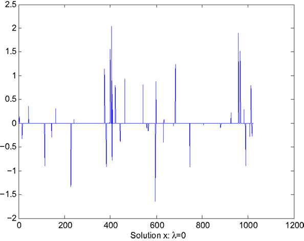
Figure 1. Solution x without sensitivity reduction: λ = 0.

We consider the sensitivity analysis and reduction for the following perturbation

$B=\mathrm{\theta }{a}_{i_0},v=\mathrm{\theta }\left[\begin{array}{c}\hfill 1\hfill \\ \hfill 0\hfill \\ \hfill ⋮\hfill \\ \hfill 0\hfill \end{array}\right]\in R^m,$ (36)

where i₀ = 959, $a_{i_0}$ is the i₀-th column of A. Note that θ is a scalar, thus p = 1. Perturbation equation (36) leads to a spike in sensitivity as shown in Figure 2. For pattern classification, each column of A represents a feature vector of a training data point. The choice of B implies that we are interested in the sensitivity of a bad training data point and seek the reduction of its effects to pattern classification. Other user-selected parameters are v = 50, τ = 0.85, η⁽ⁱ⁾ = 0.4 for all i, α₀ = 0.9, and β = 0.8. For comparison, we show the sparse solution x and the corresponding sensitivity for two cases.

FIGURE 2

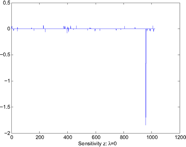
Figure 2. Sensitivity Z without sensitivity reduction: λ = 0.

Case 1: λ = 0. This case corresponds to the sparse solution to the following LASSO optimization:

$\min \tau \left|\right|x{\left|\right|}_{l_1}+\frac{1}{2}\left|\right|y-Ax{\left|\right|}_{l_2}^2.$

Figure 1 shows the values of the solution x, which clearly indicates the sparseness of the solution. Figure 2 shows the sensitivity, Z displayed in the vector form $\tilde{z}(Z=\tilde{z}\text{\hspace{0.17em}for\hspace{0.17em}}p=1)$, of x with respect to the parameter θ. The largest value of sensitivity is $\left|\right|\tilde{z}{\left|\right|}_{l_{\infty }}=1.8443$, which corresponds to x(i₀) = x(959). The largest value of sensitivity is orders of magnitude larger than the rest of sensitivity values, which indicates the solution x is sensitive to the value of the i₀th column of A.

Case 2: λ = 1.0. This case corresponds to the sparse solution with sensitivity reduction through the gradient projection algorithm described in Section 5. The values of x and $\tilde{z}$ are shown in Figures 3 and 4. Figure 3 indicates that x(i₀) is now set to 0 to remove the effect of the i₀th column of A. For pattern classification, this would mean that the feature vector corresponding to the i₀ column of A is sensitive to noise and thus is removed for this particular case. Such feature vector may be resulted from biased data or incorrect choice, depending on the particular problem of concern or scenario. The largest value of sensitivity is $\left|\right|Z{\left|\right|}_{l_{\infty }}=0.0761$, which represents orders of magnitude reduction from $\left|\right|Z{\left|\right|}_{l_{\infty }}=1.8443$.

FIGURE 3

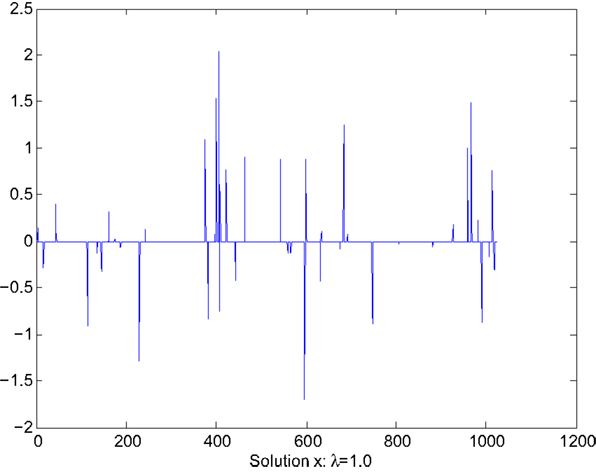
Figure 3. Solution x with sensitivity reduction: λ = 1.0.

FIGURE 4

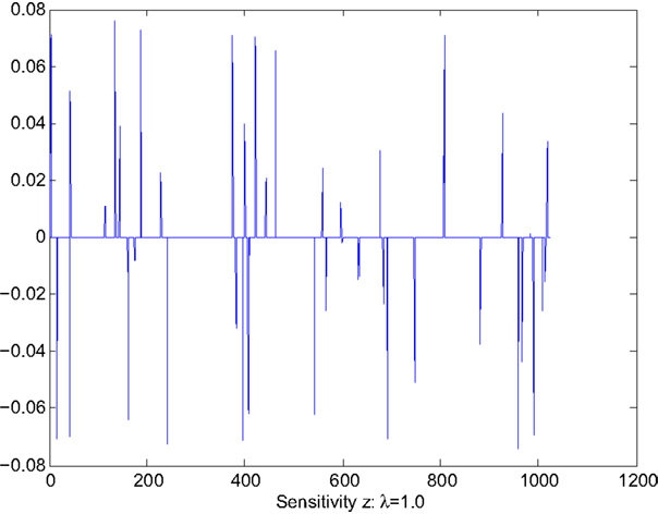
Figure 4. Sensitivity Z with sensitivity reduction: λ = 1.0.

7. Conclusion

Robustness of compressive sensing solutions has attracted extensive interest. Existing efforts have been focused on obtaining analytical bounds between the solutions of the perturbed and unperturbed linear measurement models. The perturbation is unknown but finite with a known upper bound. In this paper, we consider solution sensitivity to infinitesimal perturbations, the “other” side of perturbation has opposed to finite perturbations. The problem formulation enables the derivation of exact solutions. The results show that solution sensitivity is linear to measurement noise and proportional to the solution. We have also demonstrated how the sensitivity information can be incorporated in problem formulation to improve solution robustness. The new problem formulation provides a trade-off (i.e., by adjusting the parameter λ) between accuracy and robustness of compressive sensing solutions. One future research direction would be using the sensitivity information to adaptive optimization of parameterized compressive sensing problems. In computer vision, it is well recognized that the performance, e.g., the probability of detection, of object recognition is sensitive to feature selection and training data. The sensitivity information may be used to reduce such sensitivity, for example, in compressive sensing-based approaches to object recognition.

Conflict of Interest Statement

The author declares that the research was conducted in the absence of any commercial or financial relationships that could be construed as a potential conflict of interest.

Acknowledgments

This work is part of the author’s staff research at the North Carolina State University. The author would like to thank Prof. Dror Baron, Jin Tan, and Nikhil Krishnan for their helpful comments and constructive suggestions. Their comments lead to the correction of an error in Lemma 3.1 in an earlier version. This work is supported in part by the U.S. Army Research Office under agreement W911NF-04-D-0003.

References

Arias-Castro, E., and Eldar, Y. C. (2011). Noise folding in compressed sensing. IEEE Signal Process. Lett. 18, 478–481. doi: 10.1109/LSP.2011.2159837

CrossRef Full Text | Google Scholar

Boyd, S., Parikh, N., Chu, E., Peleato, B., and Eckstein, J. (2011). Distributed optimization and statistical learning via the alternating direction method of multipliers. Found. Trends Mach. Learn. 3, 1–122. doi:10.1561/2200000016

CrossRef Full Text | Google Scholar

Candes, E. J. (2008). The restricted isometry property and its implications for compressed sensing. C.R. Acad. Sci. Ser. I 346, 589–592. doi:10.1016/j.crma.2008.03.014

CrossRef Full Text | Google Scholar

Candes, E. J., and Romberg, J. (2005). l₁-MAGIC: Recovery of Sparse Signals via Convex Programming. Available at: http://users.ece.gatech.edu/~justin/l1magic/

Google Scholar

Candes, E. J., Romberg, J., and Tao, T. (2006). Stable signal recovery from incomplete and inaccurate measurements. Commun. Pure Appl. Math. 59, 1207–1223. doi:10.1002/cpa.20124

CrossRef Full Text | Google Scholar

Candes, E. J., and Wakin, M. B. (2008). An introduction to compressive sampling. IEEE Signal Process. Mag. 25, 21–30. doi:10.1109/MSP.2007.914731

CrossRef Full Text | Google Scholar

Chi, Y., Scharf, L. L., Pezeshki, A., and Calderbank, A. R. (2011). Sensitivity to basis mismatch in compressed sensing. IEEE Trans. Signal Process. 59, 2182–2195. doi:10.1109/TSP.2011.2112650

CrossRef Full Text | Google Scholar

Davenport, M. A., Laska, J. N., Treichler, J. R., and Baraniuk, R. G. (2012). The pros and cons of compressive sensing for wideband signal acquisition: noise folding versus dynamic range. IEEE Trans. Signal Process. 60, 4628–4642. doi:10.1109/TSP.2012.2201149

CrossRef Full Text | Google Scholar

Donoho, D., and Reevew, G. (2012). “The sensitivity of compressed sensing performance to relaxation of sparsity,” in Proceedings of the 2012 IEEE International Symposium on Information Theory (Cambridge, MA: IEEE Conference Publications), 2211–2215. doi:10.1109/ISIT.2012.6283846

CrossRef Full Text | Google Scholar

Donoho, D. L. (2006). Compressed sensing. IEEE Trans. Inf. Theory 52, 1289–1306. doi:10.1109/TIT.2006.871582

CrossRef Full Text | Google Scholar

Donoho, D. L., Elad, M., and Temlyakov, V. (2006). Stable recovery of sparse overcomplete representations in the presence of noise. IEEE Trans. Inf. Theory 52, 6–18. doi:10.1109/TIT.2005.860430

CrossRef Full Text | Google Scholar

Donoho, D. L., Maleki, A., and Montanari, A. (2011). The noise-sensitivity phase transition in compressed sensing. IEEE Trans. Inf. Theory 57, 6920–6941. doi:10.1109/TIT.2011.2165823

CrossRef Full Text | Google Scholar

Eldar, Y. C., and Kutyniok, G. (2012). Compressed Sensing: Theory and Applications. New York: Cambridge University Press.

Google Scholar

Figueiredo, M. A. T., Nowak, R. D., and Wright, S. J. (2007). Gradient projection for sparse reconstruction: application to compressed sensing and other inverse problems. IEEE J. Sel. Top. Signal Process. 1, 586–597. doi:10.1109/JSTSP.2007.910281

CrossRef Full Text | Google Scholar

Herman, M. A., and Strohmer, T. (2010). General deviants: an analysis of perturbations in compressed sensing. IEEE J. Sel. Top. Signal Process. 4, 342–349. doi:10.1109/JSTSP.2009.2039170

CrossRef Full Text | Google Scholar

Moghadam, A. A., Aghagolzadeh, M., and Radha, H. (2014). “Sensitivity analysis in RIPless compressed sensing,” in 2014 52nd Annual Allerton Conference on Communication, Control, and Computing (Allerton) (Monticello, IL: IEEE Conference Publications), 881–888. doi:10.1109/ALLERTON.2014.7028547

CrossRef Full Text | Google Scholar

Tang, Y., Chen, L., and Gu, Y. (2013). On the performance bound of sparse estimation with sensing matrix perturbation. IEEE Trans. Signal Process. 61, 4372–4386. doi:10.1109/TSP.2013.2271481

CrossRef Full Text | Google Scholar