Sensor fusion for fault detection and classification in distributed physical processes

This paper proposes a feature extraction and fusion methodology to perform fault detection and classification in distributed physical processes generating heterogeneous data. The underlying concept is built upon a semantic framework for multi-sensor data interpretation using graphical models of Probabilistic Finite State Automata (PFSA). While the computational complexity is reduced by pruning the fused graphical model using an information-theoretic approach, the algorithms are developed to achieve high reliability via retaining the essential spatiotemporal characteristics of the physical processes. The concept has been validated on a simulation test bed of distributed shipboard auxiliary systems.

1. Introduction

Sensor fusion has been one of the major focus areas in data analytics for distributed physical processes, where the individual sensory information is often used to reveal the underlying process dynamics and to identify potential changes therein. Distributed physical processes are usually equipped with multiple sensors having (possibly) different modalities over a sensor network to accommodate both model-based and data-driven diagnostics and control. The ensemble of distributed and heterogeneous information needs to be fused to generate accurate inferences about the states of critical systems in real time. Various sensor fusion methods have been reported in the literature to address the fault detection and classification problems; examples are linear and non-linear filtering, adaptive model reference methodologies, and neural network-based estimation schemes.

Researchers have used multi-layer perceptron (Liu and Scherpen, 2002) and radial basis function (Haykin, 1999) configurations of neural networks for detection and classification of plant component, sensor, and actuator faults (Napolitano et al., 2000). Hidden Markov Models and Gaussian Mixture Models are used on Multi-scale fractal dimension as features for bearing fault detection in Marwala et al. (2006). Similarly, principal component analysis (Fukunaga, 1990) and kernel regression (Shawe-Taylor, 2004) techniques have been proposed for data-driven pattern classification. These approaches address non-linear dynamics as well as scaling and data alignment issues. However, the effectiveness of data-driven techniques may often degrade rapidly for extrapolation of non-stationary data in the presence of multiplicative noise. Some of the above difficulties can be alleviated to a certain extent by simplifying approximations along with a combination of model-based and data-driven analysis as discussed below.

Robust filtering techniques have been developed to generate reliable estimations from sensor signals, because sensor time-series data are always noise-contaminated to some extent (Gelb, 1974; Grewal and Andrews, 2001). Recent literature has also reported Monte Carlo Markov chain (MCMC) techniques [e.g., particle filtering (Andrieu et al., 2004) and sigma point techniques (Julier et al., 2000)] that yield numerical solutions to Bayesian state estimation problems and have been applied to diverse non-linear dynamical systems (Li and Kadirkamanathan, 2001). The performance and quality of estimation largely depend on the modeling accuracy, which is the central problem in the filtering approach; either the dynamics must be linear or linearized, or the data must be strictly periodic or stationary for the linear models to be good estimators. It is noted that the estimation error could be considerably decreased with the availability of high-fidelity models and usage of non-linear filters, which require numerical solutions; such numerical methods are usually computationally expensive and hence may not be suitable for real-time estimation. Many techniques of reliable state estimation have been reported in literature; examples are multiple model schemes (Gopinathan et al., 1998), techniques based on analytical redundancy and residuals (Gertler, 1988), and non-linear observer theory (Garcia and Frank, 1997). Regarding sensor fusion, abnormal Patterns from Heterogeneous Time-Series have been selected via homogeneous anomaly score vectorization for Fault Event Detection (Fujimaki et al., 2009). In essence, the information from multiple sources must be synergistically aggregated for diagnosis and control of distributed physical processes (e.g., shipboard auxiliary systems).

This paper presents the development of a sensor data fusion method for fault detection and classification in distributed physical processes with an application to shipboard auxiliary systems, where the process dynamics are interactive. For example, the electrical system is coupled with hydraulic system with time-dependent thermal load. The challenge here is to mitigate several inherent difficulties that include: (i) non-stationary behavior of signals, (ii) diverse non-linearities of the process dynamics, (iii) uncertain input-output and feedback interactions and scaling, and (iv) alignment of multi-modal information and multiplicative process noise.

The sensor fusion concept, proposed in this paper, is built upon the algorithmic structure of symbolic dynamic filtering (SDF) (Ray, 2004). A spatiotemporal pattern network is constructed from disparate sensors and the fully connected network is then pruned by applying an information-theoretic (e.g., mutual information-based) approach to reduce computational complexity. The developed algorithms are demonstrated on a test bed that is constructed based on a notional MATLAB/Simulink model of Shipboard Auxiliary Systems, where a notional electrical system is coupled with a notional hydraulic system under a thermal load. A benchmark problem is created and the results under different performance metrics are presented.

The paper is organized in five sections including the present one. Section 2 presents the semantic framework for multi-sensor data modeling and explains how the proposed technique is used to prune the heterogenous sensor network for information fusion. Section 3 describes the test bed that is constructed based on a notional MATLAB/Simulink model to simulate shipboard auxiliary systems. Section 4 presents a fault injection scheme for conducting simulation exercises and validates the fault detection accuracy for different scenarios in the proposed method of information fusion. Finally, the paper is summarized and concluded in Section 5 with recommendations of future work.

2. Multi-Sensor Data Modeling and Fusion

This section presents a semantic information fusion framework that aims to capture temporal characteristics of individual sensor observations along with co-dependence among spatially distributed sensors. The concept of spatiotemporal pattern networks (STPNs) represents temporal dynamics of each sensor and their relational dependencies as probabilistic finite state automata (PFSA). Patterns emerging from individual sensors and their relational dependencies are called atomic patterns (AP) and relational patterns (RP), respectively. Sensors, APs, and RPs are represented as nodes, self-loop links, and links between pairs of nodes, respectively, in the STPN framework.

2.1. Modeling of Temporal Dynamics of Individual Sensor Data

This subsection briefly describes the concept of symbolic dynamic filtering (SDF) (Ray, 2004) for extracting atomic patterns from single-sensor data. The key concepts of SDF are succinctly presented below for completeness of the paper.

Symbolic feature extraction from time-series data is posed as a two-time-scale problem that is depicted in Figure 1. The fast scale is related to the response time of the process dynamics. Over the span of data acquisition, dynamic behavior of the system is assumed to remain invariant, i.e., the process is quasi-stationary at the fast scale. On the other hand, the slow scale is related to the time span over which non-stationary evolution of the system dynamics may occur. It is expected that the features extracted from the fast-scale data will depict statistical changes between two different slow-scale epochs if the underlying system has undergone a statistical change.

FIGURE 1

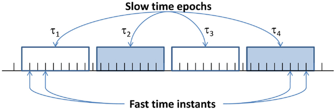
Figure 1. Notion of two-time-scale dynamics.

The algorithms of symbolic dynamic filtering (SDF) are formulated via symbolization of the time-series generated from dynamical systems along with subsequent state machine construction. The next step is the computation of the state probability vectors (or symbol generation matrices) as representatives of the statistical nature of the evolving dynamical system. To achieve this goal, the time-series data are partitioned by maximum-entropy partitioning (MEP) (Rajagopalan and Ray, 2006) to construct the symbol alphabet gma for generating symbol sequences. In this way, the information-rich regions of the time-series form finer partitioning and those with sparse information are partitioned coarser; the objective here is to maximize the Shannon entropy (Cover and Thomas, 2006) of the symbol sequence.

In the left hand corner of Figure 2, each cell is labeled by a symbol, where the alphabet of all these symbols is denoted by Σ. If Σ = {α, β, γ, δ}, then a time-series x₀, x₁, x₂… would generate a symbol sequence as: s₀, s₁, s₂…, where s_i ∈ Σ. Starting from an initial state, this mapping is called symbolic dynamic representation of the dynamical system as seen in the top right hand corner of Figure 2. The time-series data at an epoch t^k is used to compute the state-transition probabilities ${\mathrm{\pi }}_{\mathit{ij}}^k,$ of moving from state q_i to state q_j upon occurrence of a symbol, and the state probabilities $p_j^k,$ i.e., the probability of being in the state q_j at time epoch t^k. The stochastic stationary irreducible state-transition matrix is obtained as: ${\mathrm{\Pi }}^k\triangleq \left[{\mathrm{\pi }}_{\mathit{ij}}^k\right],i=1,2,\cdots ,\left|Q\right|,j=1,2,\cdots ,\left|Q\right|,$ and the corresponding state probability vector is obtained as: $p^k\triangleq \left[p_1^k,\cdots ,p_{\left|Q\right|}^k\right]$, where |Q| is the cardinality of the set Q of PFSA states, i.e., the number of PFSA states. The quasi-stationary statistics of the symbol sequence represented by the state-transition matrix Π^k at a (slow time scale) epoch t^k may evolve to Π^l at a future epoch t^l. A viable candidate for the pattern at an epoch t^k is the (|Q| × |Σ|) symbol generation matrix (also called morph matrix) ${\tilde{\Pi }}^k$ whose elements are the probabilities of symbols generated at the PFSA states. It is noted that ${\tilde{\Pi }}^k$ carries more information than the respective p ^k at the expense of higher dimensionality. The scalar-valued non-negative measure at an epoch t^k is obtained as the divergence [e.g., Euclidean distance, or Kullback–Liebler divergence (Cover and Thomas, 2006)] d(p ^k, p⁰) [resp., $d\left({\tilde{\Pi }}^k,{\tilde{\Pi }}^0\right)$] between the current pattern p ^k [resp., ${\tilde{\Pi }}^k$] from the reference pattern p⁰ [resp., ${\tilde{\Pi }}^0$] at the nominal condition denoted by the superscript “0.”

FIGURE 2

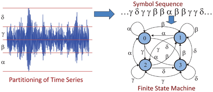
Figure 2. Construction of finite state automata (FSA) for symbolic dynamic filtering (SDF).

The core assumption in the construction of SDF is that the symbolization process under both nominal and faulty conditions is approximated as a Markov chain of order D (a positive integer), which is called the D-Markov machine. While the details of the D-Markov machine are given in Ray (2004), Adenis et al. (2012), and Li et al. (2014), the pertinent definitions and their implications are presented below.

Definition II.1. A deterministic finite state automaton (DFSA) is a 3-tuple G = (Σ, Q, δ) where (Ray, 2004; Adenis et al., 2012; Li et al., 2014):

(1) Σ is a non-empty finite set, called the symbol alphabet, with cardinality |Σ| < ∞;

(2) Q is a non-empty finite set, called the set of states, with cardinality |Q| < ∞;

(3) δ:Q × Σ→Q is the state-transition map; and Σ* is the collection of all finite-length strings with symbols from Σ including the (zero-length) empty string ε.

Remark II.1. Definition II.1 does not refer to an initial state because, in a statistically stationary setting, no initial state is required (Adenis et al., 2012).

Definition II.2. A probabilistic finite state automaton (PFSA) is constructed upon a DFSA G = (Σ, Q, δ) as a pair K = (G, π), i.e., the PFSA K is a 4-tuple K = (Σ, Q, δ, π), where (Ray, 2004; Adenis et al., 2012; Li et al., 2014):

(1) Σ, Q, and δ are the same as in Definition II.1;

(2) $\tilde{\mathrm{\pi }}:Q\times \Sigma \to \left[0,1\right]$ is the symbol generation function (also called probability morph function) that satisfies the condition ${\sum }_{\mathrm{\sigma }\in \Sigma }\tilde{\mathrm{\pi }}\left(q,\mathrm{\sigma }\right)=1\forall q\in Q,$ and π_ij is the probability of occurrence of a symbol σ_j∈Σ at the state q_i∈Q.

Definition II.3. A D-Markov machine (Ray, 2004) is a PFSA in which each state is represented by a finite history of D symbols as defined by (Ray, 2004; Adenis et al., 2012; Li et al., 2014):

• D is the depth of the Markov machine;

• Q is the finite set of states with cardinality |Q| ≤ |Σ|^D, i.e., the states are represented by equivalence classes of symbol strings of maximum length D where each symbol belongs to the alphabet Σ;

• δ:Q × Σ→Q is the state-transition function that satisfies the following condition if |Q| = |Σ|^D, then there exist α, β∈Σ and x∈Σ* such that δ(αx, β) = xβ and αx, xβ∈Q.

Remark II.2. Following Definition II.3, a D-Markov chain is a statistically stationary stochastic process S = …s₋₁, s₀, s₁… and the probability of emission of a symbol s_n depends only on the last D symbols. That is, $P\left[s_n|\cdots s_{n-D}\cdots s_{n-1}\right]=P\left[s_n|s_{n-D}\cdots s_{n-1}\right].$

The steps of D-Markov machine construction are as follows:

Step 1: State splitting to generate symbol blocks of different lengths. Words of length D on a symbol sequence qualify as the states of the D-Markov machine before the operation of state merging.

Step 2: State merging to assimilate histories from symbol blocks leading to the same symbolic behavior (Mukherjee and Ray, 2014) with a reduction in the number of states, i.e., the total number of states becomes less than or equal to |Σ|^D.

Let the state of a sensor A at the k^th instant be denoted as $q_k^A.$ With this notation, the ij^th matrix element ${\mathrm{\pi }}_{\mathit{ij}}^A$ of the (stationary) state-transition matrix Π^A is the probability that $q_{k+1}^A$ state is i given that the $q_k^A$ state was j, i.e., ${\mathrm{\pi }}_{\mathit{ij}}^A\triangleq P\left(q_{k+1}^A=i|q_k^A=j\right)$ for an arbitrary instant k.

2.2. Pattern Analysis of Multi-Sensor Information

Relational patterns (that are necessary for construction of STPN) are essentially extracted from the relational probabilistic finite state automata (PFSA). These PFSA are obtained as xD-Markov machines to determine cross-dependence as defined below; the underlying algorithm is described in Subsection 1.

2.2.1. Construction of relational PFSA: xD-Markov machine

This section describes the construction of xD-Markov machines from two symbol sequences {s₁} and {s₂} obtained from two different sensors (possibly of different modalities) to capture the symbol level cross-dependence. A formal definition is as follows:

Definition II.4. Let ℳ₁ and ℳ₂ be the PFSAs corresponding to symbol streams {s₁} and {s₂} respectively. Then a xD-Markov machine is defined as a 5-tuple ${\mathcal{M}}_{1\to 2}\triangleq \left({\mathcal{Q}}_1,{\Sigma }_1,m{a}_2,{\mathrm{\delta }}_1,{\tilde{\Pi }}_{12}\right)$ such that:

• ${\Sigma }_1=\left\{{\mathrm{\sigma }}_0,...,{\mathrm{\sigma }}_{\left|{\Sigma }_1\right|-1}\right\}$ is the alphabet set of symbol sequence {s₁};

• ${\mathcal{Q}}_1=\left\{q_1,q_2,\dots ,q_{\left|{\mathcal{Q}}_1\right|}\right\}$ is the state set corresponding to symbol sequence {s₁};

• ${\Sigma }_2=\left\{{\mathrm{\sigma }}_0,...,{\mathrm{\sigma }}_{\left|{\Sigma }_2\right|-1}\right\}$ is the alphabet set of symbol sequence {s₂};

• δ₁: 𝒬₁ × Σ₁→𝒬₁ is the state-transition mapping that maps the transition in symbol sequence {s₁} from one state to another upon arrival of a symbol in {s₁};

• ${\tilde{\Pi }}_{12}$ is the symbol generation matrix of size 𝒬₁ × Σ₂; the ij^th element of ${\tilde{\Pi }}_{12}$ denotes the probability of finding the symbol σ_j in the symbol string {s₂} while making a transition from the state q_i in the symbol sequence {s₁}.

In practice, ${\tilde{\Pi }}_{12}$ is reshaped into a vector of length 𝒬₁ × Σ₂ and is treated as the extracted feature vector that is a low-dimensional representation of the relational dependence between {s₁} and {s₂}. This feature vector is called a relational pattern (RP). When both symbol sequences are the same, RPs are essentially the atomic pattern (AP) corresponding to the symbol sequence; in that case, the xD-Markov machine reduces to a simple D-Markov machine. It is noted that an RP between two symbol sequences is not necessarily symmetric; therefore, RPs need to be identified for both directions. It is also useful to quantify cross state-transition matrices Π^AB and Π^BA to quantify the state level cross-dependence between sensors A and B. As illustrated in Figure 3, elements of the state-transition matrices Π^AB and Π^BA corresponding to the cross machines are expressed as:

$\begin{array}{llll}\hfill & {\mathrm{\pi }}_{\mathrm{k\ell }}^{\mathit{AB}}\triangleq P\left(q_{n+1}^B=\ell |q_n^A=k\right)\forall n& \hfill & \\ \hfill & {\mathrm{\pi }}_{\mathit{ij}}^{\mathit{BA}}\triangleq P\left(q_{n+1}^A=j|q_n^B=i\right)\forall n& \hfill & \end{array}$

where i, k∈Q^A and i, l∈Q^B. For a xD-Markov machine, the cross state-transition matrix is constructed from symbol sequences generated from two sensors by identifying the probability of occurrence of a state in one sensor from another state in the second sensor. For depth, D = 1 in a xD-Markov machine, a cross state-transition matrix and the corresponding cross symbol generation matrix are identical.

FIGURE 3

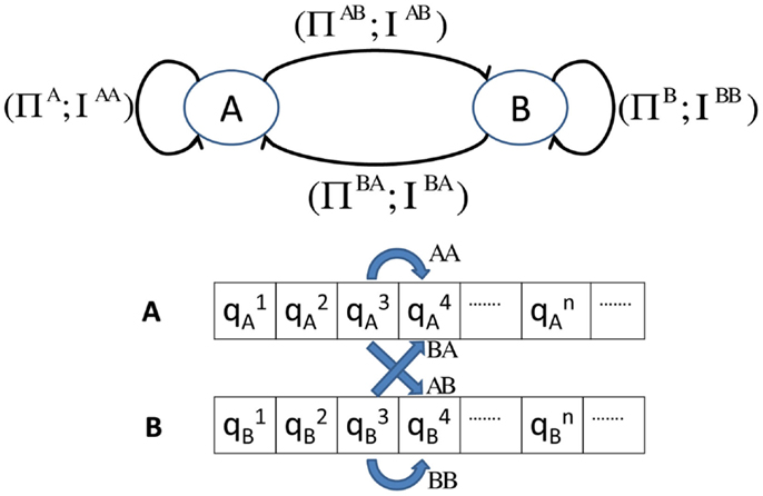
Figure 3. Illustration of Spatiotemporal Pattern Network (STPN).

2.2.2. Pruning of STPN

From the system perspectives, all APs and RPs need to be considered in order to model the nominal behaviors and to detect anomalies. However, it is obvious that there is a scalability issue if there is a significant number of sensors because the number of relational patterns increases quadratically with the number of sensors; for example, the number of RPs could be S(S-1) where S is the total number of sensors and total number of patterns become S². The explosion of the pattern space dimension may prohibit the use of a complete STPN approach for monitoring of large systems under computational and memory constraints. However, for many real systems, a large fraction of relational patterns may have a very low information content due to the lack of their physical (e.g., electro-mechanical or via feedback control loop) dependencies. Therefore, a pruning process needs to be established to identify a sufficient STPN for a system. This paper adopts an information-theoretic measure based on Mutual Information to identify the importance of an AP or an RP. Mutual information-based criteria have been very popular and useful in general graph pruning strategies (Butte and Kohane, 2000; Kretzschmar et al., 2011) including structure learning of Bayesian Networks (de Campos, 2006). In the present context, mutual information quantified on the corresponding state-transition matrix essentially provides the information contents of APs and RPs. The concept of network pruning strategy is briefly described below.

Mutual information for the atomic pattern of sensor A is expressed as:

$I^{\mathit{AA}}=I\left(q_{n+1}^A;q_n^A\right)=H\left(q_{n+1}^A\right)-H\left(q_{n+1}^A|q_n^A\right)$

where

$\begin{array}{lll}\hfill H\left(q_{n+1}^A\right)=-{\displaystyle \sum _{i=1}^{Q_A}}P\left(q_{n+1}^A=i\right){\log }_{2}P\left(q_{n+1}^A=i\right)& & \hfill \\ \hfill H\left(q_{n+1}^A|q_n^A\right)={\displaystyle \sum _{i=1}^{Q_A}}P\left(q_n^A=i\right)H\left(q_{n+1}^A|q_n^A=i\right)& & \hfill \\ \hfill H\left(q_{n+1}^A|q_n^A=i\right)=-{\displaystyle \sum _{i=1}^{Q_A}}P\left(q_{n+1}^A=l|q_n^A=i\right)\cdot & \\ \hfill {\log }_{2}P\left(q_{n+1}^A=l|q_n^A=i\right)\hfill & & \hfill \end{array}$

The quantity I^AA essentially captures the temporal self-prediction capability (self-loop) of the sensor A. However, as an extreme example, the AP for a random sensor data may not be very informative and its self mutual information becomes zero under ideal estimation.

Similarly, mutual information for the relational pattern R^AB is expressed as:

$I^{\mathit{AB}}=I\left(q_{n+1}^B;q_n^A\right)=H\left(q_{n+1}^B\right)-H\left(q_{n+1}^B|q_n^A\right)$

where

$\begin{array}{lll}\hfill H\left(q_{n+1}^B|q_n^A\right)={\displaystyle \sum _{i=1}^{Q_A}}P\left(q_n^A=i\right)H\left(q_{n+1}^B|q_n^A=i\right)& & \hfill \\ \hfill H\left(q_{n+1}^B|q_n^A=i\right)=-{\displaystyle \sum _{i=1}^{Q_B}}P\left(q_{n+1}^B=l|q_n^A=i\right)\cdot & & \hfill \\ \hfill {\log }_{2}P\left(q_{n+1}^B=l|q_n^A=i\right)\hfill & & \hfill \end{array}$

The quantity I^AB essentially captures sensor A’s capability of predicting sensor B’s outputs and vice versa for I^BA. Similar to atomic patterns, an extreme example would be the scenario where sensors A and B are not co-dependent (i.e., sensor A completely fails to predict temporal evolution of sensor B). In this case, R^AB is not very informative and I^AB will also be zero under ideal estimation.

Therefore, mutual information is able to assign weights on the patterns based on their relative importance (i.e., information content). The next step is to select certain patterns from the entire library of patterns based on a threshold on the metric. In this paper, patterns are selected based on a measure of information gain due to atomic and relational patterns. Formally, let the total information gain $I_G^{\mathit{tot}}$ is defined as the sum of mutual information for all patterns, i.e.,

$I_G^{\mathit{tot}}={\displaystyle \sum _{\left(A,B\right)\in \mathcal{S}\times \mathcal{S}}}{I}^{\mathit{AB}}$ (1)

where $\mathcal{S}$ is set of all sensors. Now, the goal is to eliminate insignificant patterns from the set $\mathcal{S}\times \mathcal{S}$ of all patterns. Let the set of rejected patterns be denoted as ${\mathcal{P}}^{\mathrm{rej}}\subset \mathcal{S}\times \mathcal{S}$ and the corresponding information gain be denoted as $I_G^{\mathit{rej}}.$ The set of rejected patterns is chosen such that, for a specified η∈(0, 1),

$\frac{I_G^{\mathit{rej}}}{I_G^{\mathit{tot}}}<\mathrm{\eta }$ (2)

where mutual information for any pattern in the reject set should be smaller than the mutual information for any pattern in the accepted set ${\mathcal{P}}^{\mathit{acc}}\triangleq \left(\mathcal{S}\times \mathcal{S}\right)\setminus {\mathcal{P}}^{\mathit{rej}},$ which is expressed as $I^{\mathit{AB}}{|}_{\left(A,B\right)\in {\mathcal{P}}^{\mathit{rej}}}\ll I^{\mathit{CD}}{|}_{\left(C,D\right)\in {\mathcal{P}}^{\mathit{acc}}}$ for a sufficiently small η. In this paper, η is chosen as 0.1 for the validation experiments. In the pruning strategy, it is possible that all patterns related to ascertain sensor might be rejected, implying that the sensor is not useful for the purpose at hand. However, the user may choose to put an additional constraint of keeping at least one (atomic or relational) pattern for each sensor in the accepted set of patterns.

Remark II.3. In order to use the STPN for fault detection, a network of PFSA can be identified following the above process under the nominal condition. Faulty conditions can then be detected by identifying the changes in parameters related to the accepted patterns. The structure of the STPN network is considered to be invariant under various health conditions of the system (i.e., nature of information content in different patterns do not change when there is a fault in the system). However, this conjecture may not hold under a very large unforeseen change in the system (i.e., a relational pattern that does not contain much information under usual circumstances may contain critical information under a large change in the system) and therefore, the STPN structure may need to change in that case. In such cases, new structures of the STPN can signify severely faulty conditions.

3. Description of Simulation Test Bed

A simulation test bed of shipboard auxiliary systems has been developed for testing the proposed algorithm of sensor fusion in distributed physical processes. The test bed is built upon the model of a notational hydraulic system that is coupled with a notional electrical system under an adjustable thermal loading.

The simulation model is implemented in MATLAB/Simulink as seen in Figure 4. This distributed notional system is driven by an external speed command ω_ref that serves as a set point for the speed, ω_e, of the permanent magnet synchronous motor (PMSM). A mechanical shaft coupling connects the fixed displacement pump (FDP) to the PMSM. The torque load of the PMSM, T_m, is obtained from the shaft model of the hydraulic system. In turn, the speed of the PMSM, ω_e, is an input to determine the angular speed of the shaft, ω_s, which drives the FDP and the cooling fan in the thermal system. In turn, the FDP drives the hydraulic motor (HM) with a dynamic load, which consists of the thermal load, T_t, and a time-varying mechanical torque load. The proportional-integral (PI) controller regulates the PMSMs electrical frequency under dynamic loading conditions that arise due to fluctuations in hydraulic and thermal loading. There is a mechanical coupling between the PMSM and the FDP of the hydraulic system, which is modeled by a rotational spring-damper system applied to an inertial load. The mechanical system outputs the shaft velocity that drives the FDP and the cooling fan of the thermal system. The pump, in turn, drives the HM through the pipeline. The HM is subjected to a time-varying load with a profile defined by the user as well as the thermal load that varies with the fan efficiency of the cooling mechanism. The systems are further coupled with a feedback loop since the torque requirement of the HM is input to the PMSM of the electrical system. The model has multiple parameters that can simulate various fault conditions. There are multiple sensors in each system with different modalities such as Hall Effect sensors, torque, speed, current, temperature, and hydraulic pressure sensors that are explained further in Section 4.

FIGURE 4

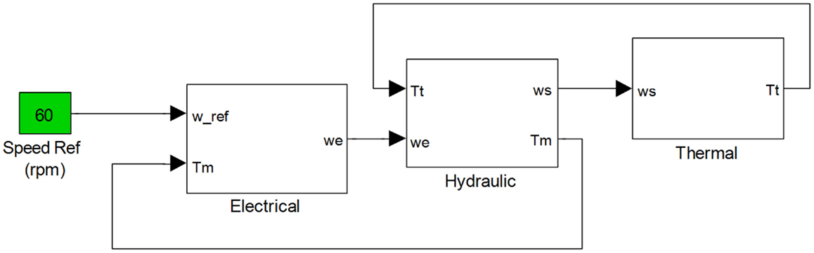
Figure 4. Notional coupled electrical, hydraulic and thermal systems.

The governing equations of the electrical component model are as follows:

$\begin{array}{llll}\hfill \frac{i_q}{\mathit{dt}}& =\frac{v_q-R{i}_q-w{L}_d{i}_d-w{\mathrm{\lambda }}_f}{L_q}& \hfill & \\ \hfill \frac{i_d}{\mathit{dt}}& =\frac{v_d-R{i}_d+w{L}_q{i}_q}{L_d}& \hfill & \\ \hfill \frac{w_r}{\mathit{dt}}& =\frac{T_e-T_l-B{w}_r}{J}& \hfill & \\ \hfill T_e& =\frac{3}{2}P\left[{\mathrm{\lambda }}_f{i}_q+\left(L_d-L_q\right)i_d{i}_q\right]& \hfill & \\ \hfill w_r& =\frac{w}{P}& \hfill & \end{array}$

where subscripts d and q have their usual significance of direct and quadrature axes in the equivalent 2-pole representation; v, i, and L are the corresponding axis voltages, stator currents, and inductances; R and ω are the stator resistance and inverter frequency, respectively; λ_f is the flux linkage of the rotor magnets with the stator; P is the number of pole pairs; T_e is the generated electromagnetic torque; T_l is the load torque; B is the damping coefficient; omega_r is the rotor speed; and J is the moment of inertia.

The governing equations of the fixed displacement pump (FDP) model are as follows:

$\begin{array}{llll}\hfill q_p& =D_p{\mathrm{\omega }}_p-k_{\mathit{leak}}{P}_p& \hfill & \\ \hfill T_p& =\frac{D_p{P}_p}{{\mathrm{\eta }}_m}& \hfill & \\ \hfill k_{\mathit{leak}}& =\frac{k_{\mathit{HP}}}{\mathrm{\nu \rho }}& \hfill & \\ \hfill k_{\mathit{HP}}& =\frac{D_p{\mathrm{\omega }}_{\mathit{nom}}\left(1-{\mathrm{\eta }}_v\right){\mathrm{\nu }}_{\mathit{nom}}\mathrm{\rho }}{P_{\mathit{nom}}}& \hfill & \end{array}$

The governing equations of the hydraulic motor (HM) model are as follows:

$\begin{array}{llll}\hfill {\mathrm{\omega }}_m& =\frac{q_m-k_{\mathit{leak}}{P}_m}{D_m}& \hfill & \\ \hfill T_m& =D_m{P}_m{\mathrm{\eta }}_m& \hfill & \\ \hfill k_{\mathit{leak}}& =\frac{k_{\mathit{HP}}}{\mathrm{\nu \rho }}& \hfill & \\ \hfill k_{\mathit{HP}}& =\frac{D_m{w}_{\mathit{nom}}\left(1-{\mathrm{\eta }}_v\right){\mathrm{\nu }}_{\mathit{nom}}\mathrm{\rho }}{P_{\mathit{nom}}}\end{array}$ (3)

where the subscripts p and m denote pump and motor parameters, respectively; the subscript nom denotes nominal values; q and P is the pressure differentials across delivery and terminal points; T is the shaft torque; D is the displacement; ω is the angular velocity; k_leak is the flow leakage coefficient; k_HP is the Hagen–Poiseuille coefficient; ν_v and ν_m are the volumetric and mechanical efficiencies, respectively; and ν and ρ are the fluid kinematic viscosity and density, respectively.

4. Results and Discussion

This section presents and discusses the results of validation of the sensor fusion algorithm on the simulation test bed.

4.1. Fault Injection, Sensors, Data Partitioning

Each of the electrical, hydraulic, and thermal subsystems of the shipboard auxiliary system is provided with a set of sensors as listed in Table 1. In the simulation test bed, selected parameters in each subsystem can be perturbed to induce faults as listed in Table 2.

TABLE 1

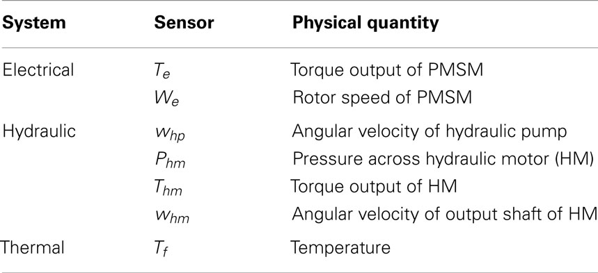
Table 1. Sensors of the system.

TABLE 2

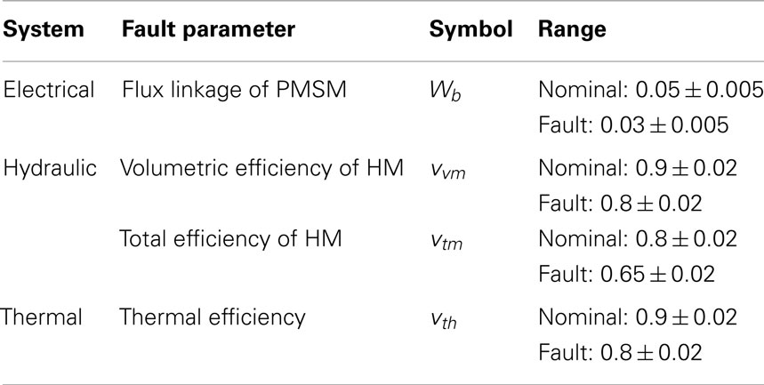
Table 2. Fault parameters of the system.

The pertinent assumptions in the execution of fault detection algorithms are delineated below:

• At any instant of time, the system is subjected to at most one of the faults mentioned in Table 2, because the occurrence of two simultaneous faults is rather unlikely in real scenarios.

• The mechanical efficiency of a hydraulic motor or a pump is assumed to stay constant over the period of observation as the degradation of machines due to wear and tear occurs at a much slower rate with respect to the drop in efficiency.

• The dynamical models in the simulation test bed are equipped with standard commercially available sensors. Exploration of other feasible sensors (e.g., ultra-high temperature sensors) to improve fault detection capabilities is not the focus of this study.

Figure 5 depicts a typical electromagnetic torque output for nominal and PMSM fault cases. As it is seen that the data itself is very noisy and, due to feedback control actions, there is no significant observable difference in the two cases in Figure 5. Information integration from disparate sensors has been performed to enhance the detection and classification accuracy in such critical fault scenarios.

FIGURE 5

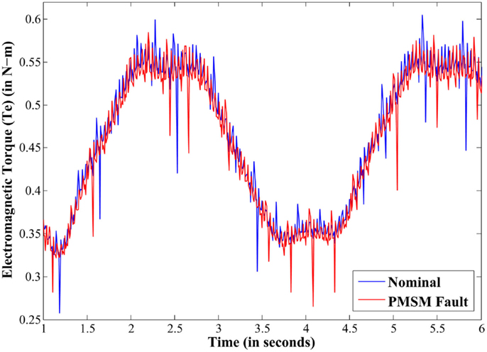
Figure 5. Electromagnetic torque under nominal and PMSM fault conditions.

For all the fault scenarios, 100 samples from each sensor are equally divided into two parts for training and testing purposes. For symbolization, maximum-entropy partitioning is used with alphabet size, |Σ| = 6 for all sensors although |Σ| does not need to be same for individual sensors. The depth for constructing PFSA states is taken to be D = 1 for construction of both atomic pattern and relational pattern. A reduced set of these patterns are aggregated to form the composite pattern, which serves as the feature classified by a k-NN classifier (with k = 5) using the Euclidean distance metric for fault detection (Bishop, 2006).

4.2. Fusion with Complete STPN

One sensor from each of the subsystems (i.e., T_f from thermal subsystem, T_e from electrical subsystem and T_hm from hydraulic subsystem) is selected for sensor fusion to identify component faults in the system. The composite patterns (CPs) are formed by concatenating atomic and relational patterns. Therefore, while patterns with high information content (based on the formulation above) help distinguishing between classes, patterns with low information content dilutes the ability of separating classes. Therefore, removing non-informative patterns may lead to reduction of both false alarm, missed detection rates, and computational complexity. In this study, CPs consist of all possible APs and RPs of T_f, T_e, and T_hm. It is seen in Table 3 that CPs perform better for detection of the nominal condition than individual sensors, but the false alarm rate is still high.

TABLE 3

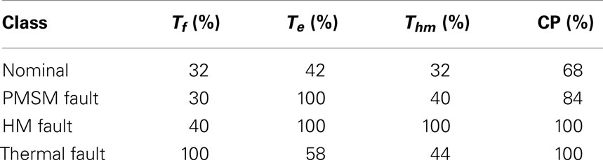
Table 3. Fault classification accuracy by exhaustive fusion.

4.3. Pruning of STPN

Pruning of large sensor networks of the given system is attempted here to reduce the complexity of fusion and improve the detection accuracy by capturing the essential spatiotemporal dynamics of the system. Left half of the Figure 6 shows a fully connected graph of seven sensors of the system where each node is a sensor; bi-directional arcs among them depict the RPs in both directions and self-loops are the APs corresponding to sensors.

FIGURE 6

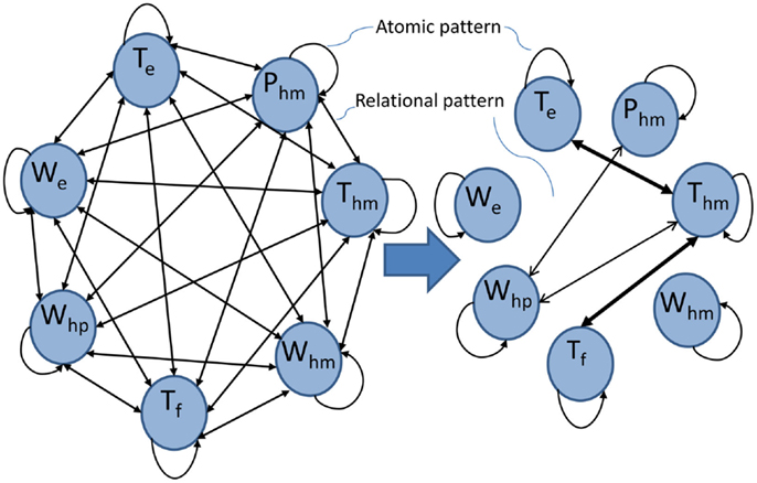
Figure 6. Pruning of STPN (Left: complete STPN, Right: pruned STPN).

The right half of Figure 6 demonstrates the pruned STPN, where the thickness of arcs represents the intensity of mutual information of the RPs among sensors. Both directions of arrows are preserved as the mutual information of the two oppositely directed RPs for a pair of sensors are comparable. In this example, all the self loops are kept intact and arcs with negligible mutual information are omitted from the graph. With higher η, the RPs (shown with thin lines in Figure 6) among w_hp, P_hm, and T_hm will not be included in the pruned network. In this simulation study, the structure of the reduced STPN is observed to remain stable for all the fault classes. The reduction in complexity of network graph is more significant in larger STPNs. The following two scenarios are chosen to justify the credibility of the pruned STPN in the light of fault detection accuracy.

4.3.1. Reduction of false alarm rates

The same set of sensors, namely, T_f, T_e, and T_hm, are selected as the STPN and it is subjected to the proposed pruning technique, which results in a composite pattern of AP of T_e $\left({\mathrm{\Pi }}^{T_e}\right)$ and two RPs (${\mathrm{\Pi }}^{T_{\mathit{hm}}{T}_e},$${\mathrm{\Pi }}^{T_{\mathit{hm}}{T}_f}$ as shown by two thick arcs in Figure 6). This action significantly reduces the false alarm rate as seen in Table 4, where APs of T_f and T_hm are dropped from the CP because these patterns do not facilitate better detection. Also PMSM fault detection accuracy does not degrade from 100% unlike fusion with complete STPN. Hence, this pruning technique reduces a CP containing 9 patterns (i.e., 3 APs, 6 RPs) to a CP of three APs and two RPs along with providing better class separability. Note, the non-informative patterns are actually acting as noise elements in the bag of patterns for the classification problem. Therefore, eliminating them from the stack is essentially analogous to increasing the signal to noise ratio, which resulted in increased accuracy of the decision system.

TABLE 4

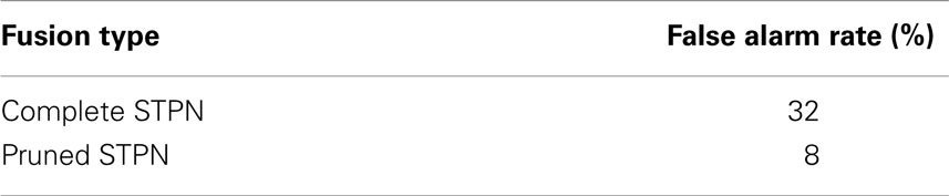
Table 4. Comparison of false alarm rate generated by exhaustive sensor fusion (complete STPN) and pruned STPN.

4.3.2. Adaptability to malfunctioning sensors

In a distributed physical process, such as the shipboard auxiliary system under consideration, malfunctioning of primary sensors in a subsystem is a plausible event. One of the current challenges in the fault detection area is to identify a fault in the subsystem with malfunctioning sensors from the sensor responses of the subsystems that are electromechanically connected. To simulate that situation, three prime heterogenous sensors from the hydraulic subsystem, namely, w_hp, P_hm, and T_hm, are selected and a fault is injected to the thermal subsystem by degrading the thermal efficiency (see Table 2). The T_f sensor of thermal subsystem is chosen to be the malfunctioning sensor and hence, it is not incorporated in the detection process of thermal fault.

As the individual sensors of the hydraulic subsystem performs rather poorly in detecting thermal faults as seen in Table 5, the information from these three sensors are fused by applying the proposed pruning technique on the hydraulic subsystem. The pruned STPN yields a CP consisting of an AP of w_hp $\left({\mathrm{\Pi }}^{w_{\mathit{hp}}}\right)$ and two RPs, namely, ${\mathrm{\Pi }}^{P_{\mathit{hm}}{w}_{\mathit{hp}}}$ and ${\mathrm{\Pi }}^{T_{\mathit{hm}}{w}_{\mathit{hp}}},$ depicted by two thin arcs in Figure 6; it results in a decent detection accuracy of 70% as seen in Table 5.

TABLE 5

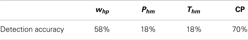
Table 5. Thermal fault detection by sensors of hydraulic subsystem.

5. Conclusion and Future Work

This paper deals with the issue of feature level fusion of multiple sensor data for data-driven fault detection techniques. The underlying algorithms are built upon the concepts of symbolic dynamic filtering (SDF) (Ray, 2004; Mukherjee and Ray, 2014) to construct a spatiotemporal pattern network from disparate sensors. The fully connected network is pruned by applying an information-theoretic approach to reduce computational complexity. In the proposed method, the abstract semantic fusion framework captures the temporal characteristics of individual sensor observations (i.e., atomic patterns) along with co-dependence among spatially distributed sensors (i.e., relational patterns) to construct a fully connected graph of the sensor network. The pruning strategy preserves the patterns having higher mutual Information to construct composite patterns that serve as the primary features for fault detection in real time. The proposed information fusion method has been validated on a test bed representing shipboard auxiliary systems. The results show that fusion with network pruning identifies component faults with a better accuracy than fusion based on the fully connected sensor network. The proposed fusion method is computationally less intensive compared to the state-of-the-art spatiotemporal fusion technique like Dynamic Bayesian Network (DBN) (Murphy, 2002) in learning phase. Moreover, compared to other sensor network pruning techniques, varied time scales of sensors of the network can be handled in an efficient way by STPN construction in the proposed technique. The pattern generation technique (SDF) is also compared extensively to the benchmark feature extraction techniques in Rao et al. (2009) and Bahrampour et al. (2013) and found to have comparable or better performance in anomaly detection and classification along with higher computational efficiency. However, the objective function of the pruning operation does not involve classification accuracy explicitly. Therefore, comparison of the current objective function with a classification-oriented objective function remains an important future work. Although, the classification performance may get better with such an objective function, computational complexity, and data availability may become issues as it will become a supervised pruning scheme as opposed to the current un-supervised scheme. Apart from this task, the following research areas are recommended as topics of future investigation:

• Optimization of the threshold of ratio of mutual information η (Section 2) subjected to better fault detection and lesser complexity.

• Rigorous testing of robustness (e.g., using boosting schemes) of the pruning strategy over different fault types and classes.

• Validation of the fusion algorithm on larger sensor network of real distributed systems.

• Comparison between developed method and other state-of-the-art network pruning and fusion algorithm (both model-driven and data-driven) for fault detection.

• Comparison with other types of classifiers for the same pruned network.

Conflict of Interest Statement

The authors declare that the research was conducted in the absence of any commercial or financial relationships that could be construed as a potential conflict of interest.

Acknowledgments

This work has been supported in part by US Navy contract no. N00014-M-12-0055. Any opinions, findings, and conclusions or recommendations expressed in this publication are those of the authors and do not necessarily reflect the views of the sponsoring agencies.

References

Adenis, P., Wen, Y., and Ray, A. (2012). An inner product space on irreducible and synchronizable probabilistic finite state automata. Math. Control Signals Syst. 23, 281–310. doi: 10.1007/s00498-012-0075-1

CrossRef Full Text | Google Scholar

Andrieu, C., Doucet, A., Singh, S., and Tadic, V. B. (2004). Particle methods for change detection, system identification, and control. Proc. IEEE 92, 423–438. doi:10.1109/JPROC.2003.823142

CrossRef Full Text | Google Scholar

Bahrampour, S., Ray, A., Sarkar, S., Damarla, T., and Nasrabadi, N. M. (2013). Performance comparison of feature extraction algorithms for target detection and classification. Pattern Recognit. Lett. 34, 2126–2134. doi:10.1016/j.patrec.2013.06.021

CrossRef Full Text | Google Scholar

Bishop, C. M. (2006). Pattern Recognition and Machine Learning. New York, NY: Springer.

Google Scholar

Butte, A. J., and Kohane, I. S. (2000). “Mutual information relevance networks:functional genomic clustering using pairwise entropy measurements,” in Pacific Symposium on Biocomputing (Island of Oahu, Hawaii), 418–429.

Google Scholar

Cover, T., and Thomas, J. (2006). Elements of Information Theory, 2nd Edn. New York, NY: Wiley.

Google Scholar

de Campos, L. M. (2006). A scoring function for learning Bayesian networks based on mutual information and conditional independence tests. J. Mach. Learn. Res. 7, 2149–2187.

Google Scholar

Fujimaki, R., Nakata, T., Tsukahara, H., Sato, A., and Yamanishi, K. (2009). Mining abnormal patterns from heterogeneous time-series with irrelevant features for fault event detection. Stat. Anal. Data Min. 2, 1–17. doi:10.1002/sam.10030

CrossRef Full Text | Google Scholar

Fukunaga, K. (1990). Statistical Pattern Recognition, 2 Edn. Boston, MA: Academic Press.

Google Scholar

Garcia, E. A., and Frank, P. M. (1997). Deterministic nonlinear observer-based approaches to fault diagnosis: a survey. Control Eng. Pract. 5, 663–670. doi:10.1016/S0967-0661(97)00048-8

CrossRef Full Text | Google Scholar

Gelb, A. (ed.) (1974). Applied Optimal Estimation. Cambridge, MA: The MIT Press.

Google Scholar

Gertler, J. J. (1988). Survey of model-based failure detection and isolation in complex plants. IEEE Control Syst. Mag. 8, 3–11. doi:10.1109/37.9163

CrossRef Full Text | Google Scholar

Gopinathan, M., Boskovic, J. D., Mehra, R. K., and Rago, C. (1998). “A multiple model predictive scheme for fault-tolerant flight control design,” in Conference on Decision and Control (Tampa, FL), 1376–1381.

Google Scholar

Grewal, M. S., and Andrews, A. P. (2001). Kalman Filtering: Theory and Practice Using MATLAB, 2 Edn. New York: John Wiley & Sons.

Google Scholar

Haykin, S. (1999). Neural Networks: A Comprehensive Foundation. Upper Saddle River, NJ: Prentice Hall.

Google Scholar

Julier, S., Uhlmann, J., and Durrant-Whyte, H. F. (2000). A new method for the nonlinear transformation of means and covariances in filters and estimators. IEEE Trans. Automat. Contr. 45, 477–482. doi:10.1109/9.847726

CrossRef Full Text | Google Scholar

Kretzschmar, H., Stachniss, C., and Grisetti, G. (2011). “Efficient information-theoretic graph pruning for graph-based slam with laser range finders,” in International Conference on Intelligent Robots and Systems (IROS) (San Francisco, CA), 865–871.

Google Scholar

Li, P., and Kadirkamanathan, V. (2001). Particle filtering based likelihood ratio approach to fault diagnosis in nonlinear stochastic systems. IEEE Trans. Syst. Man Cybern. 31, 337–343. doi:10.1109/5326.971661

CrossRef Full Text | Google Scholar

Li, Y., Shen, Z., Ray, A., and Rahn, C. (2014). Real-time estimation of lead-acid battery parameters: a dynamic data-driven approach. J. Power Sources 268, 758–764. doi:10.1016/j.jpowsour.2014.06.099

CrossRef Full Text | Google Scholar

Liu, J., and Scherpen, J. M. A. (2002). Fault detection method for nonlinear systems based on probabilistic neural network filtering. Int. J. Syst. Sci. 33, 1039–1050. doi:10.1080/0020772021000046216

CrossRef Full Text | Google Scholar

Marwala, T., Mahola, U., and Nelwamondo, F. (2006). “Hidden Markov models and Gaussian mixture models for bearing fault detection using fractals,” in Proceedings of International Joint Conference on Neural Networks (Vancouver, BC), 3237–3242.

Google Scholar

Mukherjee, K., and Ray, A. (2014). State splitting and merging in probabilistic finite state automata for signal representation and analysis. Signal Processing 104, 105–119. doi:10.1016/j.sigpro.2014.03.045

CrossRef Full Text | Google Scholar

Murphy, K. P. (2002). Dynamic Bayesian Networks: Representation, Inference and Learning. Ph.D. thesis, University of California, Berkeley, CA.

Google Scholar

Napolitano, M. R., An, Y., and Seanor, B. A. (2000). A fault tolerant flight control system for sensor and actuator failures using neural networks. Aircr. Des. 3, 103–128. doi:10.1016/S1369-8869(00)00009-4

CrossRef Full Text | Google Scholar

Rajagopalan, V., and Ray, A. (2006). Symbolic time series analysis via wavelet-based partitioning. Signal Processing 86, 3309–3320. doi:10.1016/j.sigpro.2006.01.014

CrossRef Full Text | Google Scholar

Rao, C., Ray, A., Sarkar, S., and Yasar, M. (2009). Review and comparative evaluation of symbolic dynamic filtering for detection of anomaly patterns. Signal Image Video Process. 3, 101–114. doi:10.1007/s11760-008-0061-8

CrossRef Full Text | Google Scholar

Ray, A. (2004). Symbolic dynamic analysis of complex systems for anomaly detection. Signal Processing 84, 1115–1130. doi:10.1016/j.sigpro.2004.03.011

CrossRef Full Text | Google Scholar

Shawe-Taylor, J. (2004). Kernel Methods for Pattern Analysis. Cambridge: Cambridge University Press.

Google Scholar