Spatiotemporal variability of chlorophyll-a concentration in the South Brazil Bight using 25 years of multi-sensor orbital data (1998–2022)

Chlorophyll-a (Chl-a) concentration is a key climate variable, as its variability is associated with meteorological and oceanographic processes. This study analyzed 25 years (1998–2022) of Chl-a data from the European Space Agency (ESA) Ocean Colour Climate Change Initiative (OC-CCI) multisensor archive for the South Brazil Bight, Southwestern Atlantic. Temporal variability and trends were assessed using the Census X11 method, Mann-Kendall, and Sens’ slope tests. The ESA OC-CCI data highlight reliable regional performance, although Chl-a concentrations above 10 mg.m⁻³ were underestimated. Temporal analyses showed the lowest Chl-a variability (29%) in open ocean waters, with 81% of the variability attributed to seasonal dynamics influenced by the South Atlantic Subtropical Gyre (SASG). A negative Chl-a trend of −11.0% was observed over the 25-year period, attributed to the expansion of the oligotrophic area of the SASG. In the shelf areas southwest of São Sebastião Island, Chl-a variability was moderate (34%–39%), with no discernible long-term trend, but significant interannual variability (44%). The Cape Frio upwelling region shows an increasing Chl-a trend (14.5% in the last 25 years), driven by atmospheric circulation affecting local winds. The highest Chl-a variability (74%) occurred along the southern continental shelf, associated with seasonal nutrient inputs from the Subtropical Shelf Front, with a Chla-a trend increase of 7.5% in 25 years. These results highlight the dynamic and variable Chl-a responses to environmental forcing across the South Brazil Bight.

1 Introduction

Chlorophyll-a (Chl-a) concentration is classified as an Essential Climate Variable by the World Meteorological Organization and the Global Climate Observing System (GCOS, 2021). It serves as an indicator of total phytoplankton biomass, a key parameter for monitoring the trophic status of aquatic environments (Cael et al., 2023) and the response of marine ecosystems to changes due to modulation of environmental conditions associated with climate or human influences (Rabalais et al., 2009). A clear diagnostic of the current status and recent changes in the biogeochemical properties of marine ecosystems is a pre-requisite to support current efforts to develop sustainable management of global (UNESCO-IOC, 2021; IPCC, 2023) and regional (CGEE, 2022) marine waters.

Focusing on Ocean Color Remote Sensing (OCRS) observations, medium to low spatial resolution (300 m–1 km) satellite archives now provide information over a sufficiently long time period (daily continuous data since 1997) to characterize the response of ocean waters to environmental changes at different time scales (interannual changes, seasonal modulations, episodic events) (IPCC, 2023). International efforts have been developed to generate long and consistent remotely sensed ocean color time series by merging the satellite sensors into a unique dataset (IOCCG, 2007). Among the multi-sensor projects that ensure operational continuity and accessibility, data from the Ocean Colour Climate Change Initiative (OC-CCI) (Sathyendranath et al., 2019; Jackson et al., 2022) are currently the only merged products available globally at 1 km resolution and were therefore considered in the current study.

The study of 25 years of temporal variation combined with 1 km spatial resolution of satellite chlorophyll-a (Chl-a_sat) estimates from multi-sensor data over the South Brazil Bight (SBB), SW Atlantic, represents an innovative and unmet challenge. However, to fully exploit the potential of global Chl-a_sat, regional quality-control of the data is required prior to time series analysis. The quality of the Chl-a_sat allows a robust temporal analysis, where temporal variations are considered as a response to environmental changes rather than as a potential limitation of the algorithm used (Mélin et al., 2017; Sathyendranath et al., 2017). While many studies have documented the performance of Chl-a algorithms (O’Reilly and Werdell, 2019; Lavigne et al., 2021; Tilstone et al., 2021; Tran et al., 2023; Werdell et al., 2023) with several studies evaluating the SBB for mono-sensor applications (Garcia et al., 2005; Kampel et al., 2007; Carvalho et al., 2014; Oliveira et al., 2016; Cesar et al., 2023), more regional evaluations of the merged datasets are still required.

The South Brazil Bight is a dynamic zone influenced by seasonal hydrographic (Castro, 2014) and biogeochemical (Brandini et al., 2018) processes. The circulation of the shelf currents, forced by changes in the wind, promotes the intrusion of cold, nutrient-rich water, which is essential for phytoplankton growth (Castro et al., 2006). The outer shelf and shelf break are influenced by the water masses transported by the Brazil Current, whose meanders and eddies promote nutrient-rich water intrusion (Campos et al., 2000; Silveira et al., 2020). Large river and estuarine discharges, such as those from the La Plata River and Patos Lagoon, contribute to the remote fertilization of the shelf region (Garcia and Garcia, 2008; Gonçalves-Araujo et al., 2018). The variability of Chl-a in the SBB is intrinsically linked to changes in these atmospheric and oceanographic processes. Comprehending these environmental modulations is essential for understanding the structure and dynamics of marine ecosystems.

Previous studies in the SBB based on long-term ocean color time series are relatively scarce. For example, Ciotti et al. (2010) analyzed the seasonal and interannual variation of Chl-a_sat over the SBB using 12 years of data from the Sea-viewing Wide Field-of-view Sensor (SeaWiFS). They found no increase or decrease in Chl-a_sat concentration over time, treating the SBB as a single, homogeneous region, despite its dynamic spatial and temporal characteristics. The authors also noted the limited observation period as a limitation for trend analysis. Therefore, a pixel-based, long-term analysis of Chl-a_sat over the SBB is still needed to capture patterns at smaller spatial and larger temporal scales to provide insights to better understand Chl-a concentration variations and climate-related impacts.

In this context, this study aims to analyze the spatial and temporal variability of Chl-a_sat estimates in the SBB over 25 years and their possible relationship with environmental changes. For this purpose, the daily OC-CCI Chl-a_sat product (1998–2022) was evaluated by comparisons with in situ Chl-a measurements. The respective daily OC-CCI R_rs(λ) spectrum was used to classify each matchup point taking into account the Optical Water Type (OWT) classification (Mélin and Vantrepotte, 2015). The Chl-a_sat performance assessment was the basis for applying the Census X11 decomposition method and long-term trend analysis in a quality-controlled Chl-a_sat dataset. The Chl-a_sat observations were analyzed by applying adapted statistical methods, including monotonic trend detection (Hirsch et al., 1982) and time series decomposition techniques, to describe the dominant patterns of temporal variability and to assess the shape of the observed changes in Chl-a_sat concentrations over the past 25 years (Vantrepotte and Mélin, 2009; 2011).

2 Materials and methods

2.1 Study area

The SBB is located in the subtropical western South Atlantic and extends in latitude from Cape São Tomé (22° S) to Cape Santa Marta (28.5° S) (Figure 1). The shelf break is associated with the 180 m isobath, with the widest shelf extension occurring in the central region (160 km on average), in contrast to the narrower northeastern shelf (60 km long on average) (Mahiques et al., 2010). At Cape Frio ($\sim$23° S), the coastline abruptly shifts from North-South to East-West direction. Changes in bottom topography and shoreline orientation contribute to upwelling events in the region (Rodrigues and Lorenzzetti, 2001; Calado et al., 2010).

Figure 1

Figure 1. (A) Location of the South Brazil Bight (red triangle) on the map of South America, with the borders of Brazil highlighted (grey shading). (B) Currents and water masses. Red arrow: the Brazil Current which transports the Tropical Water (surface) and the South Atlantic Central Water (SACW) at depth. Light blue curved arrow: the SACW inshore intrusion over the SBB shelf. Dark blue arrow: the Brazilian Coastal Current, which transports the Subtropical Shelf Front. (C, D) are satellite estimates of OC-CCI multi-sensor monthly mean surface chlorophyll-a concentrations over the South Brazil Bight during (C) austral summer (January) and (D) austral winter (July) of 2007. From the coast to the open ocean, the thin black lines are the 50, 100, and 180 m isobaths. The white circles labeled P1 to P4 are representative sites of the open ocean waters (P1), the Cape Frio upwelling system (P2), the interannual variability of São Sebastião Island (P3), and the Subtropical Shelf Front (P4) discussed in the text. Acronyms along the coast are referenced in the figure legend.

The SBB is influenced by three water masses: the Tropical Water (TW), the South Atlantic Central Water (SACW), and the Coastal Water (CW) (Emílsson, 1961; Peterson and Stramma, 1991; Castro et al., 2006). Each of these water masses is characterized by specific thermohaline characteristics (and thus nutrient contents). The TW (salinity >36 psu; temperature >20°C) and the SACW (salinity between 34.6 psu and 36 psu; temperature <20°C) are transported southward by the Brazil Current (BC) at depths between 0–150 m and 150–500 m, respectively (Silveira et al., 2020). The CW has a low salinity characteristic as it corresponds to continental water inputs combined with TW and SACW mixing. It can be present in coastal parts north of the SBB shelf, from Cape Frio to São Sebastião Island, and in large cross-shelf extensions south of the SBB shelf (Braga and Niencheski, 2006; Fries et al., 2019; Marta-Almeida et al., 2021; Dottori et al., 2023; Silva et al., 2023; Braga et al., 2024). The contribution of water masses varies throughout the year, depending on the seasonal modulation of atmospheric and oceanographic processes.

During the austral summer, local east-northeast winds are responsible for a wind-driven Ekman transport of surface CW and TW waters offshore, making way for SACW intrusion (Castro, 2014). Where the continental shelf is narrow, such as at Cape Frio and Cape Santa Marta, SACW intrusion can reach the surface under favorable E-NE wind conditions (Castelao and Barth, 2006). Three days of 10 m.s⁻¹ northeasterly winds could bring the SACW to the surface along the Cape Frio coast (coastal upwelling), greatly increasing Chl-a concentrations (e.g. from 0.01 mg.m^-3–5.6 mg.m^-3 as shown in Gonzalez-Rodriguez et al. (1992)). The nutrient-rich upwelling water can remotely fertilize the shelf flowing from its core to the southwest, transported by the wind-driven coastal current and the Brazil Current (Valentin, 2001; Brandini et al., 2018; Calil et al., 2021).

The onshore position of the Brazil Current (BC) during the summer season (Lorenzzetti et al., 2009) can intensify the subsurface intrusion of the SACW over the shelf (Coelho-Souza et al., 2012; Castro, 2014). As the conservation of vorticity activity changes due the topography and shoreline orientation, the BC generates cyclonic and anticyclonic meanders and eddies (Campos et al., 2000; Silveira et al., 2000), which may lead to shelf break upwelling and support the coastal upwelling events of SACW (Campos et al., 2000; Calado et al., 2010; Coelho-Souza et al., 2012). When the TW is present in the upper layer, an oligotrophic condition is observed with average Chl-a values around 0.21 mg.m⁻³ over the SBB, varying from 0.13 mg.m⁻³ offshore to 0.46 mg.m⁻³ on the shelf (Kampel, 2003; Gaeta and Brandini, 2006). Along the coast, the Chl-a concentration has a year-round average value of $\sim$ 2.9 mg.m⁻³, induced by continental inputs to the CW and shallower depths providing nutrients to the euphotic zone (Gaeta and Brandini, 2006).

During winter, while the frequency of southwesterly winds and the northward intrusion of cold fronts coming from the south increases (Piola et al., 2000; Pimenta et al., 2005; Oliveira and Kampel, 2019; Bodnariuk et al., 2021), the South Atlantic Subtropical High (SASH), which corresponds to northeasterly winds, moves further north and east (Pezzi et al., 2022; Dottori et al., 2023). The passage of cold fronts creates turbulence in the vertical structure of the water masses over the shelf, supplying nutrients that enhance Chl-a levels throughout the year (Gaeta et al., 1999), especially in winter when the thermocline stratification is weaker (Castro, 2014). The South Atlantic Subtropical Gyre (SASG) is also retreating toward the equator, bringing the BC front together. These processes favor the intrusion of the La Plata Plume Water (PPW), which is associated with colder, nutrient-rich Sub-Antarctic Water and the Patos/Mirim Lagoon plumes across the shelf. The combination of these waters is referred to as the Subtropical Shelf Front (SSF) and moves along the inner-middle shelf of the SBB, carried by the Brazil Coastal Current (Piola et al., 2000; de Souza and Robinson, 2004). Under the influence of the nutrient-rich SSF, the Chl-a concentration increases with values higher than 2.0 mg.m⁻³ (Brandini, 1990). Higher surface Chl-a concentrations are also observed over the SBB replacing the oligotrophic conditions typical of summer, with average values of 0.23 mg.m⁻³ offshore and 0.96 mg.m⁻³ on the shelf (Kampel, 2003).

2.2 In situ and satellite data sets

A compilation of in situ surface (<2 m depth) Chl-a measurements (hereafter Chl-a_insitu) collected in the SBB waters was performed considering multiple cruises (Supplementary Table S1) for regional satellite validation exercises. The samples of Chl-a_insitu measurements used in this study were collected from 1998 to 2022 combining the same period of the satellite Chl-a dataset. The methodologies used to calculate the Chl-a_insitu concentrations varied according to the data source (e.g., HPLC, fluorometry, and spectrophotometry). The methodological details are described in the respective references (Supplementary Table S1).

Daily multi-sensor merged OC-CCI remote sensing reflectance (R_rs(λ)) spectra and the Chl-a_sat archives from January 1998 to December 2022 were downloaded from the European Space Agency (ESA) website (https://climate.esa.int/en/projects/ocean-colour/data/) in its version 6.0. The OC-CCI data source was used because of its long time series availability of more than 25 years (September 1997 – present) of Level 3 daily data in a gridded cell size of 1 km spatial resolution and cloud masked.

For the R_rs(λ), the input data set is the combination of SeaWiFS, Moderate Resolution Imaging Spectroradiometer (MODIS), Medium Resolution Imaging Spectrometer (MERIS), Visible Infrared Imaging Radiometer Suite (VIIRS), and Ocean and Land Color Instrument (OLCI). The SeaWiFS sensor is atmospherically corrected using the NASA l2gen, while the other sensors use POLYMER (Steinmetz et al., 2011). The Level 2 product of each sensor is masked by applying the IDEPIX cloud and land masks (all sensors), the NASA L2 flags (for SeaWiFS), and the POLYMER bitmask (for MODIS, MERIS, VIIRS, and OLCI). The masked Level 2 of SeaWiFS, MODIS, and VIIRS sensors are band shifted to MERIS nominal bands (λ = 412, 443, 490, 510, 560, and 665 nm) by first computing the inherent optical properties (IOPs) of each sensor using the quasi-analytical algorithm inversion model (Lee et al., 2002), and second using the IOPs to calculate the R_rs(λ) in the MERIS bands for each sensor (Jackson et al., 2022). The band shift of each sensor is adjusted using a bias correction and all individual sensors are merged with a simple average to produce the final OC-CCI R_rs product. The merged R_rs bands are used to calculate the Chl-a_sat estimate based on empirical Color Index (CI) and blue/green band ratio algorithms such as OCI, OCI2, OC2, and OCx (Werdell et al., 2023). All the Chl-a_sat algorithms are merged and weighted according to the OC-CCI water type classification (Moore et al., 2009).

To map the extent of the SSF intrusion, daily Multiscale Ultrahigh Resolution (MUR) Sea Surface Temperature (SST) was used to generate monthly averages of SST for July and August 2007. The SST dataset was obtained from the Physical Oceanography Distributed Active Archive Center (PO.DAAC) website (https://podaac.jpl.nasa.gov/dataset/MUR-JPL-L4-GLOB-v4.1) with a spatial resolution grid of 1 km in its Level 4 (JPL MUR MEaSUREs Project, 2015).

2.3 OC-CCI Chl-a_sat validation

A matchup validation exercise was performed by extracting the OC-CCI Chl-a_sat over a 3 × 3 pixel window centered on the location of each station composing the Chl-a_insitu data set. Chl-a_sat averages were then calculated for each subset using standard quality control criteria. In practice, matchup data were selected based on criteria requiring at least 5 valid pixels to ensure the spatial representativeness of each subset and a maximum coefficient of variation of 25% for Chl-a_sat values, excluding data with high spatial heterogeneity (Kahru et al., 2014; Concha et al., 2021). Since OC-CCI data are a composite of multiple sensors, it is not possible to evaluate performance within a time window of hours. The time window criterium for matchup was defined as the same day between satellite imagery and in situ sampling.

Classical statistical descriptors were used to evaluate the performance of the OC-CCI Chl-a_sat estimates at the regional scale. All statistical analyses were performed on the log-transformed Chl-a data (in situ and satellite) due to its log-normal distribution in oceanic waters (Campbell, 1995). These include the bias for identifying systematic differences, the Root Mean Square Difference (RMSD), the coefficient of determination (r²), and the slope and intercept of the linear regression line between log₁₀(Chl-a_sat) and log₁₀(Chl-a_insitu) (Bailey and Werdell, 2006). The Median Absolute Percent Difference (MAPD) was also calculated using the log-transformed dataset and analyzed as the percentage error of the log₁₀(Chl-a_sat) estimate. An overview of the statistical descriptor equations was attached in the Supplementary Equations S1–S4.

2.4 Optical water type (OWT) classification

OWT classification was performed on the OC-CCI R_rs(λ) spectra extracted at the same 3 × 3 pixel window locations and dates as the Chl-a_sat matchups. The mean R_rs(λ) for each 3 × 3 pixel window was calculated using the same criteria applied to the Chl-a_sat data (≥5 valid pixels and ≤25% variance). The normalized R_rs(λ) was obtained by dividing each R_rs(λ) by the integral of the R_rs spectrum from 412 nm to 665 nm, considering linear interpolation between the nominal wavelength center bands based on the MERIS sensor. Each normalized R_rs spectrum was then assigned to one of the 17 global OWT classes defined by Mélin and Vantrepotte (2015) and updated by Jorge et al. (2021). For this, a multivariate probability density function was calculated for each normalized R_rs spectrum and the 17 OWTs references using the Python package “scipy” v.1.13. The higher probability of similarity between the R_rs spectrum and an OWT class was taken into account. This classification method was also applied to the monthly R_rs(λ) composite images on a pixel-by-pixel basis to analyze the spatial distribution of OWTs over the SBB from 1998 to 2022.

2.5 Time series analysis

For time series analyses, monthly composites for Chl-a_sat and R_rs(λ) were generated using the corresponding daily OC-CCI data from January 1998 to December 2022. The geometric mean was applied, which is less sensitive to extreme values, meaning that outliers or a small number of Chl-a_sat and R_rs(λ) samples may have a significantly smaller impact on the results of the time series analysis. The monthly Chl-a_sat time series was decomposed on a pixel-by-pixel basis using the Census X11 method (Pezzulli et al., 2005). As described in detail in Vantrepotte and Mélin (2011), this iterative analysis involves the successive application of bandpass filters to decompose the time series into three additive components: seasonal, irregular (sub-annual), and interannual variability. The Census X11 method needs a regular continuous time series. In cases where the pixel has <25% representativeness along the 300 months (25 years), the Census X11 interpolates the gaps according to the method described in Ibanez and Conversi (2002). Otherwise, for the pixels with >25% gaps, the Census X11 excludes the entire data and masks the respective pixel along the time-series analysis, avoiding a non-fiducial interpolation of missing data (Vantrepotte and Mélin, 2009). The interest in this method for accurately describing temporal variation patterns has been demonstrated in various ocean color-based studies at regional or global scales (Beaulieu et al., 2013; Loisel et al., 2014; Keerthi et al., 2022). In addition to visualizing the temporal patterns associated with the extracted time series, the Census X11 output allows to display the relative importance (in %) of the three components to the total variance of the series.

The non-parametric seasonal Mann-Kendall test (Hirsch et al., 1982) with a statistical probability threshold of 0.05 (p < 0.05) was applied to the monthly Chl-a_sat time series to identify increasing or decreasing trends in specific regions. The magnitude of existing monotonic trends was calculated using the seasonal Sen’s slope method (Sen, 1968). The Python package “pymannkendall” version 1.4.3 (Hussain and Mahmud, 2019) was used for the seasonal Mann-Kendall and seasonal Sen’s slope statistical tests. The Pruned Exact Linear Time computational cost method (Killick et al., 2012) was used to detect the change points based on the mean of the monthly Chl-a_sat interannual signal time series observations. This method is implemented in the Matlab package “findchangepts” in its version available in R2020a. A minimum distance of 12 steps (1 year) was set between the change points, since the input data is the interannual signal of monthly Chl-a_sat.

3 Results

3.1 OC-CCI chlorophyll-a validation

A total of 185 matchups were obtained with Chl-a_insitu concentrations ranging from 0.1 to 351.5 mg.m⁻³ and a mean value of 25.5 mg.m⁻³. The mean concentration of Chl-a_sat estimates was 9.8 mg.m⁻³ with a minimum of 0.1 mg.m⁻³ and a maximum that did not exceed 32.5 mg.m⁻³ (Table 1). The OC-CCI Chl-a_sat was retrieved with a satisfactory accuracy up to about 10 mg.m⁻³, where an underestimation of the Chl-a_sat values was found. The respective R_rs(λ) spectrum of the Chl-a_sat concentrations above the threshold of 10 mg.m⁻³, corresponded to samples belonging to OWTs 1 and 2 (Figure 2).

Table 1

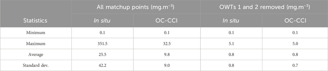
Table 1. Statistical comparison (in mg.m⁻³) between in situ and OC-CCI Chl-a matchup points with all OWT classes and removing OWTs 1 and 2.

Figure 2

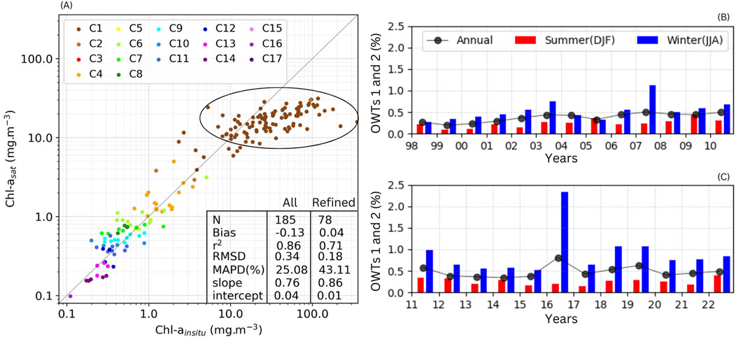
Figure 2. (A) Scatter plot of Chl-a matchups with statistical performance (in log scale). Colors represent the OWT classification for each sample, from turbid (C1) to oligotrophic (C17) waters. The black ellipse represents the Chl-a_sat limit corresponding to some classes 1 and 2 matchups. The table columns refer to all matchup points (“All”) and after removal of OWTs 1 and 2 (“Refined”). (B, C) are the annual and seasonal percentage areas of OWTs 1 and 2 compared to the total area of the SBB from 1998 to 2010 (B) and 2011–2022 (C).

When OWTs 1 and 2 were removed from the matchup validation, the statistics showed better agreement between the Chl-a_insitu and Chl-a_sat with similar values for minimum, maximum, average, and standard deviation (Table 1). In general, the Chl-a_sat performance also showed an improvement in results after removing pixels from OWTs 1 and 2 (Figure 2). The number of samples decreased to 78 out of 185, however the bias decreased from −0.13 to 0.04, and the RMSD improved from 0.34 to 0.18. The regression line parameters had a better fit to the data (slope = 0.86, intercept = 0.01). Spatially, the in situ samples belonging to OWTs 1 and 2 were observed mainly inside Guanabara Bay and Sepetiba Bay (Figure 3).

Figure 3

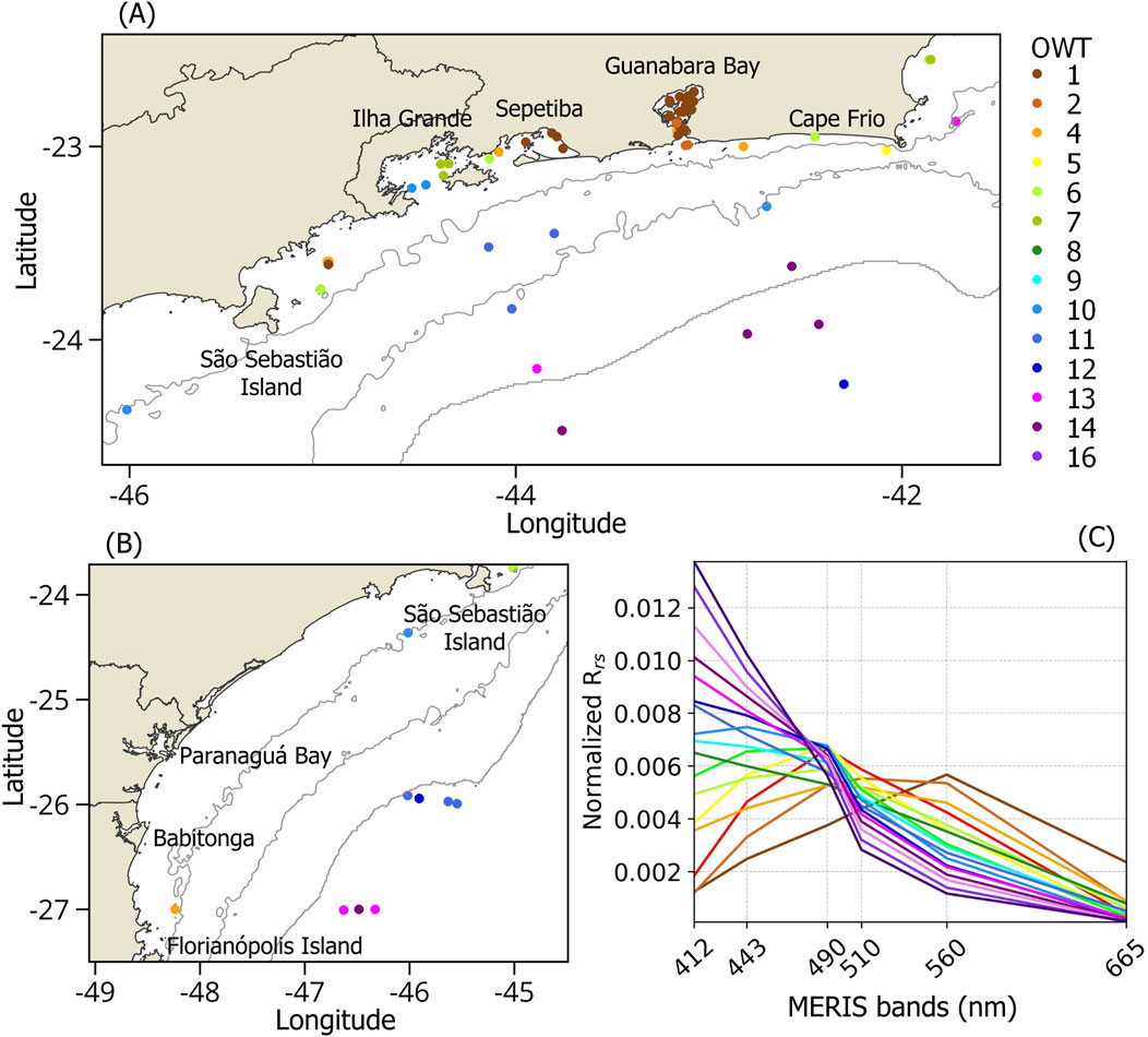
Figure 3. Spatial distribution of Chl-a_insitu and Chl-a_sat matchup points and the corresponding OWT classes in colors from Cape Frio to São Sebastião Island (A) and from São Sebastião Island to Florianópolis Island (B). From the coast to the open ocean, the thin gray lines are the 50, 100, and 180 m isobaths. (C) OWTs normalized spectra from classes C1 (turbid) to C17 (oligotrophic) adapted from Jorge et al. (2021).

A pixel-based classification was done in the monthly OC-CCI R_rs(λ) images to identify the areas where OWTs 1 and 2 were present. Overall, OWTs 1 and 2 represent less than 1% of the total valid pixels in the study area and are more present during the winter season (Figure 2). Episodic events with a higher frequency of OWTs 1 and 2 coincide with the northernmost position of the SSF associated with PPW discharge and southerly winds. The OWTs 1 and 2 were throughout the year in estuaries, bays, and coastal areas (Supplementary Figure S1). These include areas such as Guanabara Bay, Sepetiba Bay, Santos Estuary, Cananeia-Iguape Estuary-Lagoon Complex, Paranaguá Bay, Babitonga Bay, and the coastal waters between Santos Estuary and Florianópolis Island influenced by continental inputs (Marta-Almeida et al., 2021). In practice, since the Chl-a_sat performance is biased for concentrations above 10 mg.m⁻³, the following analysis, Sections 3.2, 3.3 were performed using the Chl-a_sat time series from 1998 to 2022, after excluding the pixels classified as OWTs 1 and 2. The number of available daily data for each month and year used to perform further spatial and temporal analysis is described in Supplementary Table S2–S5.

3.2 Spatial Chl-a_sat variability

Four regions of interest were selected as representative of different temporal variability patterns based on the amplitude of the Chl-a_sat coefficient of variation (CV, %) and temporal variability patterns highlighted by the relative contribution of the Census X11 components (irregular, seasonal and interannual, in %, Figure 4) to the total variance of the Chl-a_sat signal from 1998 to 2022. These regions were also combined with the trend analysis criterium calculated by the Mann-Kendall and Sen’s slope tests to define areas where Chl-a_sat showed a significant increase or decrease over the 25 years.

Figure 4

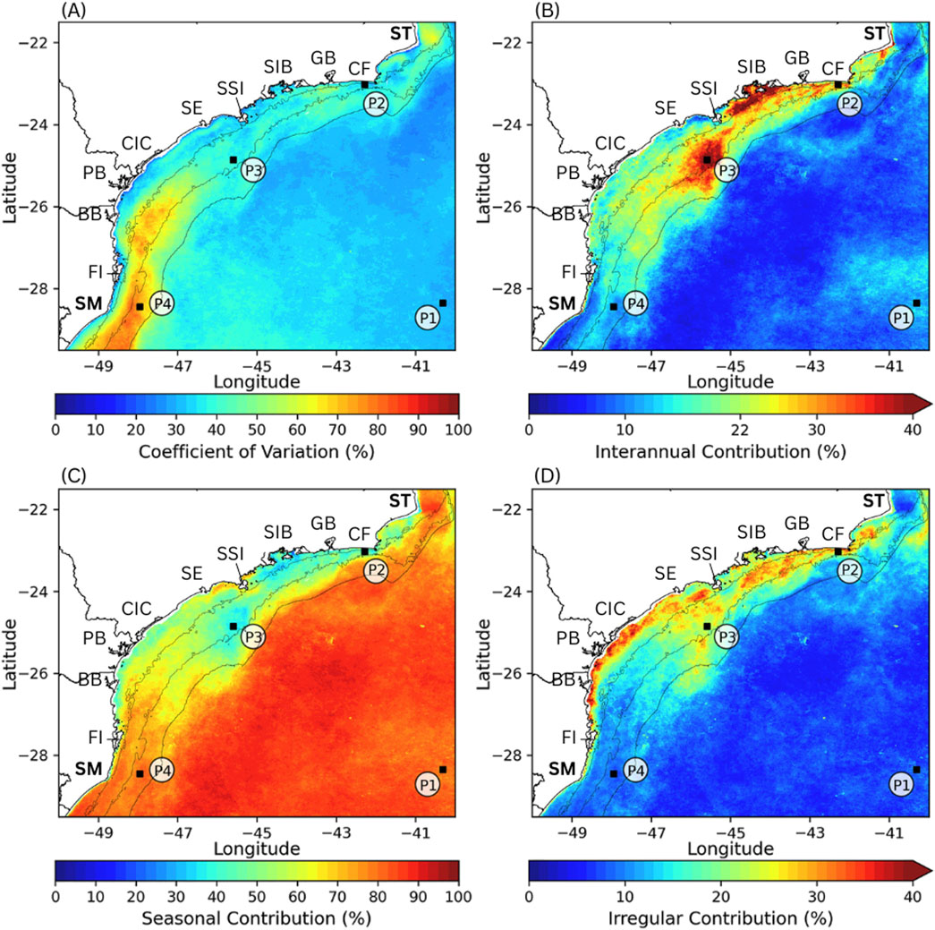
Figure 4. (A) Chl-a_sat coefficient of variation (%). Analysis of the relative contribution of the interannual (B), seasonal (C), and irregular (D) Census X11 components to the total variation of the Chl-a_sat time series over the period 1998-2022. The white circles labeled from P1 to P4 are representative sites of the open ocean (P1), the Cape Frio upwelling system (P2), the São Sebastião Island interannual variation (P3), and the Subtropical Shelf Front (P4) discussed in the text. From the coast to the open ocean, the thin black lines are the 50, 100, and 180 m isobaths. A list of region names and their respective acronyms is given in Figure 1.

Exercises using different coverage sizes were conducted over the four regions of interest, and it was found that a 5 × 5 pixel window best elucidated the different patterns over the SBB. As observed in Supplementary Figure S1, the 5 × 5 pixel windows sites are not located over the pixels classified as OWTs 1 and 2 where the Chl-a_sat algorithm limitations and the gaps after removing OWTs 1 and 2 could affect the analysis. In this way, monthly Chl-a_sat concentration averages of 5 × 5 pixel windows identified from P1 to P4 were extracted and used to explain the different patterns identified in the four regions of interest over the SBB.

Open ocean waters (P1 site) associated with the SASG show relatively low temporal variability with CV values lower than 30% (Figure 4A). In these oceanic water masses, the seasonal cycle globally controls most of the temporal variation of the Chl-a_sat. This is illustrated by the statistics extracted for P1, where 81% of the total variance of the Chl-a_sat concentration (ranging from 0.04 mg.m⁻³ to 0.18 mg.m⁻³) can be attributed to seasonal modulations (Table 2).

Table 2

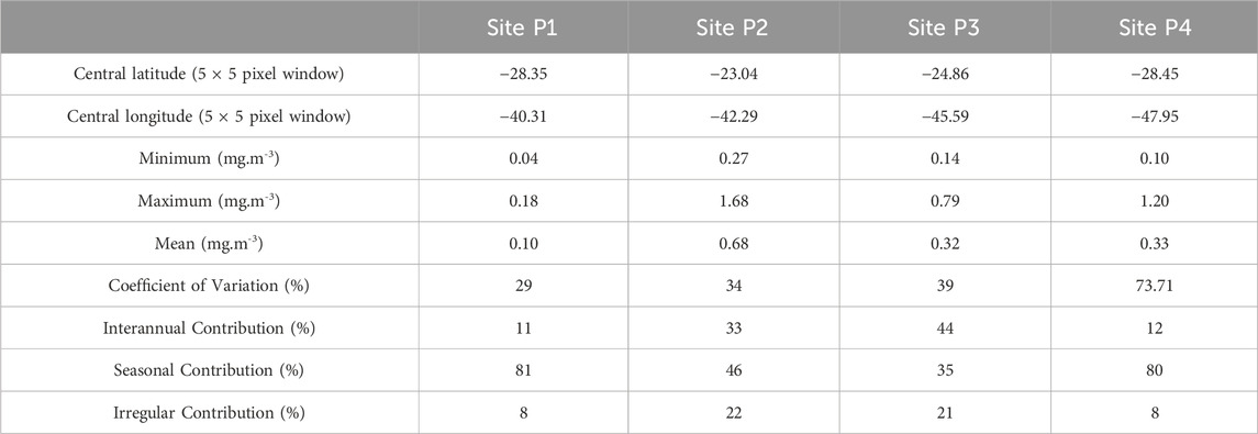
Table 2. Statistics of the monthly Chl-a_sat concentration values (minimum, maximum, and mean) and the results of the Census X11 decomposition analysis for the coefficient of variation (CV) and the contribution of the interannual, seasonal, and irregular components at the four sites (P1 to P4) identified in Figure 4.

In contrast to the pattern shown for the oceanic waters, the northern and central regions of the SBB shelf, from Cape Frio to the latitude of Paranaguá Bay (23° S–25° S), show a heterogeneous temporal CV variability ranging from 30% to 50%. In the Cape Frio sector (P2), where coastal upwelling occurs, the Chl-a_sat CV is 34%, with minimum and maximum monthly Chl-a_sat concentrations between 0.27 mg.m⁻³ and 1.68 mg.m⁻³, respectively. The contribution of the Census X11 components to the total variance of the series is globally balanced, with 33%, 43%, and 24% associated with the interannual (Figure 4B), seasonal (Figure 4C), and irregular (Figure 4D) terms, respectively. The southwest of São Sebastião Island (P3) has a monthly Chl-a_sat concentration between 0.14 mg.m⁻³ and 0.79 mg.m⁻³ (CV = 39%). In this area, a dominance of the interannual variation is found (44% of the total variation of the series) followed by the seasonal (35%) and irregular (21%) variations (Table 2).

From 25° S to the south (between 50 and 180 m isobaths), influenced by the SFF, the Chl-a_sat CV ranges from 50% to 84% (Figure 4A). This high variability is mainly related to the contribution of the seasonal component (Figure 4C). In P4, representative of the southern region of the SBB continental shelf, the CV is 74% with Chl-a_sat concentrations ranging from 0.10 mg.m⁻³ to 1.2 mg.m⁻³, and 80% of the variance of the series is explained by the seasonal pattern.

3.3 Chl-a_sat seasonal pattern and trend analysis

At site P1, the monthly Chl-a_sat climatology shows lower values during the austral summer and higher values during the winter (Figure 5A). During the austral summer, north-northeasterly winds favor the SASG area of low Chl-a_sat concentrations to expand south-southeastward with warmer SST intensifying the vertical stratification of the water column. The processes that occur during the summer (December to February) do not make the nutrients in the mixed layer available for phytoplankton assimilation. In winter (June to August), southerly winds favor the retreat of the SASG to the north-northwest, which is replaced by cooler waters, reducing vertical stability. This displacement of the mixed layer into deeper waters tends to increase nutrient availability, which promotes phytoplankton primary production and biomass growth (McClain et al., 2004; Signorini et al., 2015).

Figure 5

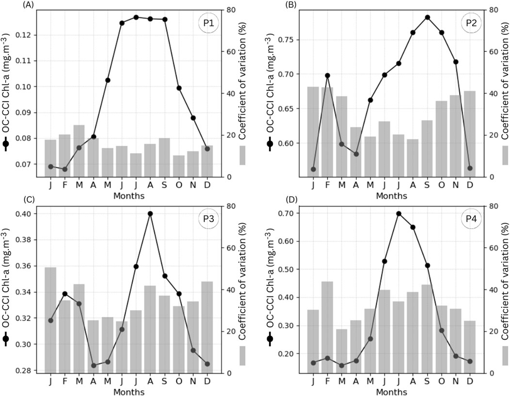
Figure 5. Monthly climatology of Chl-a_sat concentration (mg.m⁻³) between 1998 and 2022 at sites P1 (A), P2 (B), P3 (C), and P4 (D) and the Chl-a_sat coefficient of variation. Note that the Chl-a_sat y-axis has different scales.

The high Chl-a_sat concentration during the summer season in the climatological analysis at P2 (Figure 5B) and P3 (Figure 5C) is related to the SACW upwelling in the Cape Frio region (P2) and the SACW intrusion in P3. The winds from the first quadrant (north-northeast) are present throughout the year but predominate during the summer season (Cerda and Castro, 2014), favoring the Ekman transport of surface waters offshore and the SACW intrusion over the shelf. At P3, the SACW intrusion does not necessarily reach the surface (Brandini et al., 2014), although vertical mixing influenced by surface (wind) and bottom (SACW intrusion) stress can occur. Nevertheless, satellite observations can capture the high Chl-a_sat concentration in the subsurface, as this maximum occurs at the first optical depth in the water column (i.e., ≥37% of the incident light) (IOCCG, 2019; Nababan et al., 2021).

The higher Chl-a_sat CV at P2 during summer (about 40%) compared to the winter months of the climatological analysis may be related to the frequency and persistence of short-term phytoplankton blooms. For example, in the Cape Frio region (P2), upwelling episodes lasting 2 days and a rapid increase in biomass from 0.01 to 5.6 mg.m⁻³ were observed (Gonzalez-Rodriguez et al., 1992). The variability of the surface Chl-a_sat concentration during the summer months in this area is related to the amount and duration of the upwelling events as shown by the CV values higher than 40%. During the winter, in the absence of favorable winds, the surface Chl-a_sat remains stable and the CV maintains around 20%.

High surface Chl-a_sat concentrations during the winter time period for the P2 and P3 have been already reported in previous studies (Kampel, 2003; Ciotti et al., 2010). During winter, the northeasterly winds weaken and southerly winds dominate, while the Brazil Current retreats, carrying the TW and SACW off the shelf (Silveira et al., 2000). The southerly winds generate vertical turbulence in the shelf water, which tends to homogenize the water column (Castro, 2014), introducing nutrients into the euphotic layer (Brandini et al., 2018) and promoting an increase in phytoplankton biomass. The P4 site is also influenced by the northward intrusion of the nutrient-rich SSF (Piola et al., 2000; Brandini et al., 2018). The SSF can also occasionally reach the northern part of the SBB, such as site P3, transported by the Brazilian Coastal Current (BCC). Figure 6 shows the long range of the SSF intrusion in 2007 following the 19°C–20°C isotherm up to site P3. Cross-correlation analysis between monthly Chl-a_sat concentrations at P3 and P4 showed an increase in phytoplankton biomass with a 1-month delay (first peak in P4 followed by P3). Zavialov et al. (2002) found average values of BCC velocity along-shore of 16 cm.s⁻¹, which corresponds to a northward SSF intrusion of 414 km.month⁻¹. This is the approximate distance between P4 and P3, confirming the Chl-a_sat cross-correlation result and the influence of the SSF intrusion driven by BCC northward flow at both sites in some episodic events.

Figure 6

Figure 6. Subtropical Shelf Front (SSF) buoyancy advection in July (A) and August (B) of 2007. The dark blue line contour is the 19°C isotherm and the light blue is the 20°C isotherm. Sites P1 to P4 are labeled in (A) and represented by black squares in both images. A list of region names and their respective acronyms is given in Figure 1.

In addition to the seasonal variation previously described from the 25-year monthly climatology, an analysis of the Census X11 time series was conducted to more accurately describe Chl-a dynamics in different areas of the SBB, taking into account episodic events and interannual variation in seasonal patterns and average Chl-a_sat values. At P1, the seasonal oscillation is evident with Chl-a_sat peaks in winter, in agreement with the observed climatology (Figure 5). The change point detection applied to the Census X11 interannual term at the P1 site shows the presence of a regime shift in August 2011 with a 10% decrease in the Chl-a_sat mean (from 0.10 mg.m⁻³ to 0.09 mg.m⁻³). This is consistent with the results of the monotonic trend analysis, which shows the presence of a significant (p < 0.05) decrease (−0.44%.year⁻¹, −11% over the 25 years) in the Chl-a_sat time series (Figure 7). The size of the oligotrophic area of the SASG, warmer SST, and changes in the meridional and extratropical atmospheric circulation are possible drivers for the decrease in the Chl-a_sat concentration (Vantrepotte and Mélin, 2011; Signorini et al., 2015).

Figure 7

Figure 7. Census X11 time series decomposition at site P1, representative of oceanic waters. (A) Monthly Chl-a_sat concentrations. (B) The interannual signal (black line) and the monotonic trend (red line). The vertical grey bars indicate the change points in the Chl-a_sat average detected in the interannual signal and the Chl-a_sat average before and after the change point (dashed grey line). (C) The seasonal and irregular signals. The x-axis labels are years from 01/1998 to 12/2022 and the x-ticks are located in January of each year.

Over the Cape Frio upwelling region (P2), the monthly Chl-a_sat concentration shows small temporal scale (sub-annual) variations (Figure 8A), as also underlined by the relatively high contribution of the irregular component (22%) to the total variance of the Chl-a_sat (Figure 4). These small-scale variations observed in the irregular signal (Figure 8C) could be related to episodic and irregular phytoplankton blooms induced by the influence of favorable local northeasterly winds (Gonzalez-Rodriguez et al., 1992; Valentin, 2001). The trend analysis indicates the presence of a significant (p < 0.05) monotonic increase of 0.58%.year⁻¹ (i.e. 14.5% in the past 25 years) in this area. The change detection analysis shows that this increasing trend is more likely associated with the presence of a tipping point in the mean Chl-a_sat between August 2011 and October 2012 (Figure 8B). Splitting the time series before and after 2011-2012, the Chl-a_sat shows a significant increase from 1998 to 2011 with an average of 0.64 mg.m⁻³, a peak in Chl-a_sat between 2011 and 2012 with the Chl-a_sat value reaching 1.0 mg.m⁻³, and a significant decreasing trend in Chl-a_sat, returning to an average value of 0.68 mg.m⁻³ from 2012 to 2022.

Figure 8

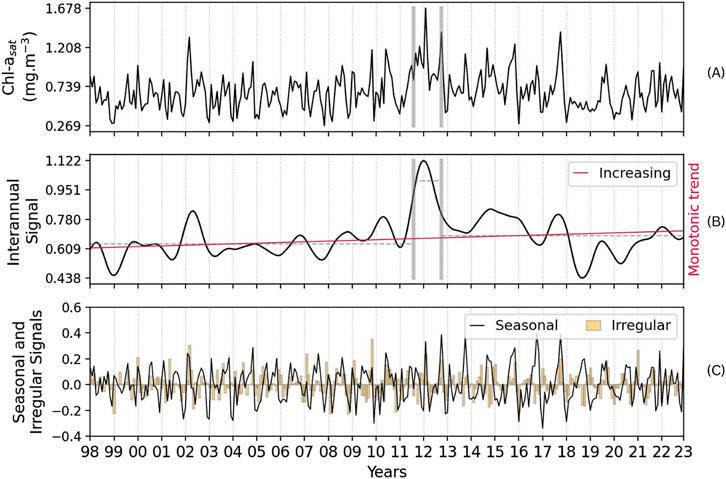
Figure 8. Census X11 time series decomposition at site P2, representative of the Cape Frio upwelling system. (A) Monthly Chl-a_sat concentrations. (B) The interannual signal (black line) and the monotonic trend (red line). The vertical grey bars indicate the change points in the Chl-a_sat mean detected in the interannual signal and the Chl-a_sat mean before and after the change point (dashed grey line). (C) The seasonal and irregular signals. The x-axis labels are the years from 01/1998 to 12/2022 and the x-ticks are located in January of each year.

The tipping point identified in the Chl-a_sat averages in August 2011 at points P1 (Figure 7) and P2 (Figure 8) indicates an inverse correlation between the two regions, probably related to changes in the atmospheric and oceanic circulation (Yang et al., 2023; Xing et al., 2024). At P1, the interannual component of Chl-a_sat shows a decrease until 2011 (p < 0.05) and then an increase from 2014 (p > 0.05). Conversely, the Cape Frio upwelling system at P2 increased until 2011 and then showed a decrease in Chl-a_sat averages from 2012 onwards. Over the 25-year series, both sites show inverse long-term patterns in the Chl-a_sat with significant decreasing trends at P1 and increasing trends at P2.

At P3, located in the southwest of São Sebastião Island, no significant trend in Chl-a_sat was detected (p > 0.05), although considerable interannual variability was observed, as indicated by four change points from 1998 to 2022 (Figure 9). The average Chl-a_sat concentrations during the periods 1998–2004 (0.35 mg.m⁻³), 2007–2012 (0.33 mg.m⁻³) and 2015–2022 (0.31 mg.m^-3) were very similar to the overall average for P3 (0.35 mg.m⁻³) from 1998 to 2002. In contrast, a significantly lower average Chl-a_sat of 0.23 mg.m⁻³ was recorded between 2004 and 2007, while a higher average of 0.45 mg.m⁻³ was recorded from 2012 to 2014. This combination of lower (2004–2007) and higher (2012–2014) Chl-a_sat values, together with low variability during other periods, explains the lack of significant trends over the entire OC-CCI timeframe (1998–2022). It also highlights the importance of accurately representing nonlinear interannual patterns, which can be masked by simple trend analysis.

Figure 9

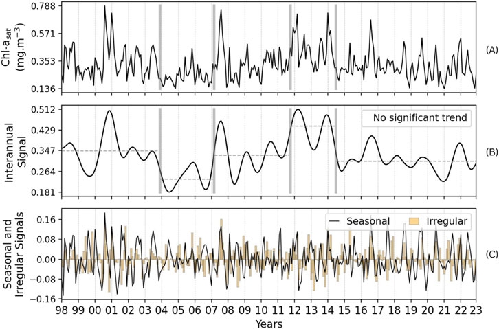
Figure 9. Census X11 time series decomposition at site P3, representative of the southwest of São Sebastião Island (A) Monthly Chl-a_sat concentrations. (B) The interannual signal (black line). The vertical grey bars indicate change points in the Chl-a_sat mean detected in the interannual signal and the Chl-a_sat mean before and after the change point (dashed grey line). (C) The seasonal and irregular signals. The x-axis labels are years from 01/1998 to 12/2022 and the x-ticks are located in January of each year.

The southern part of the SBB shelf (site P4) shows a significant (p < 0.05) Chl-a_sat increase of 0.3% per year (7.5% in 25 years) (Figure 10). This region shows a well-defined seasonal cycle, with elevated Chl-a_sat values during the winter throughout the 25-year period. While no change points were detected in the interannual Chla term, five local maxima (in 2000, 2003, 2007, 2013, and 2016) followed by five local minima (in 2001, 2004, 2008, 2014, and 2017) can be identified. These variations are related to the El Niño-Southern Oscillation (ENSO) phase which affects the SSF volume and, in combination with atmospheric wind changes, drives the SSF northwards over the SBB shelf, as indicated by the extension of the cold-water plume observed on the SST maps (<20°C) in Figure 6. Similar interannual patterns are observed for P3 and P4 (correlation coefficient of 0.53), mainly due to the comparable signal responses during the aforementioned maximum and minimum years mentioned above. This suggests that the aforementioned influence of ENSO anomalies can also affect the P3 site, as highlighted by the high contribution of the interannual variability to the total variance of the Chl-a_sat observed in the south of São Sebastião Island.

Figure 10

Figure 10. Census X11 time series decomposition at site P4, representative of the southern SBB shelf influenced by seasonal SSF intrusion. (A) Monthly Chl-a_sat concentrations. (B) The interannual signal (black line) and the monotonic trend (red line). (C) The seasonal and irregular signals. The x-axis labels are years from 01/1998 to 12/2022 and the x-ticks are located in January of each year.

4 Discussion

4.1 OC-CCI chlorophyll-a assessment

Matchup analysis of the OC-CCI Chl-a_sat product in the SBB identified a major limitation: it underestimates Chl-a_insitu above 10 mg.m⁻³, whose concentration is however rarely reached in the area. For example, Kampel et al. (2007) evaluated the performance of the algorithms for the SeaWiFS sensor using the Chl-a dataset, which includes 117 samples over the SBB and found maximum concentrations of about 3.00 mg.m⁻³. Carvalho et al. (2014) compared 49 Chl-a_insitu samples near the Santos Estuary, reporting mean concentrations of 2.46 mg.m⁻³ and a low frequency of values above 10 mg.m⁻³ in inner shelf waters, with spectral shapes typical of turbid waters. Brandini et al. (2014) found Chl-a_insitu concentrations ranging from 0.07 to 6.2 mg.m⁻³ in a transect at latitude −26.7° S, sampling along the 20–180 m isobaths. Cesar et al. (2023) analyzed 15 years of monthly surface Chl-a_insitu measurements done in the 40 m isobath northeast of São Sebastião Island (23.60° N – 44.97° W) and found an average Chl-a of 1.0 mg.m⁻³, with episodic events reaching up to 18 mg.m⁻³.

The limitation of the Chl-a_sat estimates is associated with pixels classified as OWTs 1 and 2, which represent less than 1% of the total pixels imaged in the SBB (Figure 2). Considering the spatial pixel-by-pixel classification of the monthly R_rs(λ) spectra, this 1% is located in bays, lagoons, estuaries, and coastal regions influenced by continental inputs (Supplementary Figure S1). In turbid or high Chl-a coastal waters, it is necessary to use the information provided in the red and near-infrared (NIR) portion of the R_rs signal due to the influence of non-algal particle reflectance and phytoplankton absorption and fluorescence processes at the longest visible wavelengths. In enclosed bays and estuaries, high concentrations of colored dissolved organic matter can obscure the phytoplankton Chl-a signal at shorter wavelengths of the R_rs spectrum, which are typically used in blue-green band ratio algorithms (Neil et al., 2019; Lavigne et al., 2021; Tran et al., 2023). Thus, the use of the OC-CCI Chl-a_sat product remains feasible for broader studies over the entire SBB shelf, but should be avoided for studies in the coastal environment where Chl-a concentrations can often exceed 10 mg.m⁻³.

The current OC-CCI catalog does not provide the R_rs in the NIR, which limits the application of Chl-a_sat inversion models specifically designed for turbid or high Chl-a coastal waters, such as those used in the matchup analysis. In the context of monitoring high Chl-a values using satellite data, two options are currently available, each with inherent limitations. The first option is to use a mono-sensor time series; the MODIS sensor on board the Aqua satellite currently provides the longest continuous ocean color time series. However, the NASA Ocean Biology Processing Group (OBPG) recently reported a degradation in the radiometric quality of the MODIS sensor in early 2023, which is expected to continue to worsen (Twedt et al., 2023). Consequently, the longest available time series from a single ocean color data source is limited to 20 years of MODIS data (2002–2022) until a potential recalibration for the 2023 dataset is implemented.

The second option is to use the merged products, which do not include the necessary enhancements for coastal environments, such as the availability of the NIR band and Chl-a algorithms that incorporate the NIR band into the Chl-a_sat merged product. According to the OC-CCI project User Guide, the upcoming OC-CCI version (v7.0) will use the OLCI sensor bands as the default central wavelengths, but there is no mention of the implementation of the NIR bands so far (Jackson et al., 2022). This new version will also include any sensor reprocessing updates before June 2023, which will not address the degradation of MODIS data. In both scenarios, atmospheric corrections developed for turbid-eutrophic waters should be applied as described in IOCCG (2024), as well as the validation of the products for these higher Chl-a coastal values is also essential as applied in previous studies (Lavigne et al., 2021; Tran et al., 2023). It remains essential to assess the suitability of merged products compared to mono-sensor time series (Mélin et al., 2017; Sathyendranath et al., 2017).

Of the 17 OWTs describing the optical diversity of global marine waters, as documented by Jorge et al. (2021) and complementing the initial classification by Mélin and Vantrepotte (2015) for global coastal waters (16 classes), 12 were observed at a regional scale, with classes 3, 5, 8, 15, and 17 missing. The validation of the OC-CCI Chl-a product in this study does not fully represent the regional diversity; for example, OWT 17 was identified in the open ocean waters of the SBB during the austral summer season, but there are no matchup data for validation in this region highlighting the need to further develop validation in the region.

4.2 Chl-a_sat dynamics in the SBB over the past 25 years

The long-term trend of Chl-a_sat over the oligotrophic waters of the ocean gyres has been studied without a general agreement between increase (McClain et al., 2004; Aiken et al., 2017; Hammond et al., 2020; Cael et al., 2023) or decrease (Vantrepotte and Mélin, 2011; Signorini et al., 2015). The opposite trend observed between studies is mainly related to the spatiotemporal coverage. For example, Ciotti et al. (2010) performed a monotonic trend analysis over the entire South Brazil Bight using a regional average time series, for which no significant trend was observed. This may be due to compensation of increasing and decreasing trend patterns within the large region selected by the authors. In other cases, such as in McClain et al. (2004) and Hammond et al. (2020), the integration of the full SASG may lead to increasing trends. Another point is the number of years used in previous studies and the need for long-term observations (Henson et al., 2010; Mélin et al., 2017). For example, if this study had used a time series starting from 2012 (10 years), the monotonic trend observed would be different (and in some cases as sites P1 and P2 opposite) than that observed with 25 years of data.

At site P1, the decrease in the Chl-a_sat concentration (−0.48%.y⁻¹) follows the trend observed by Vantrepotte and Mélin (2011) and Signorini et al. (2015). Vantrepotte and Mélin (2011) calculated the monotonic trend in the southwestern region of the SASG, which is representative of site P1. They found a decreasing trend up to −1.0%.y⁻¹ using 10 years of data from the SeaWiFS sensor. Signorini et al. (2015) combined SeaWiFS and MODIS sensors in a 16-year time series and found a decreasing trend of −0.30% and −0.23%.y⁻¹ in Chl-a_sat estimated using the standard and Ocean Color Index algorithms, respectively.

The decrease in open ocean Chl-a_sat concentrations observed in these studies is associated with the increasing trend of SST in the South Atlantic (Polovina et al., 2008; Johnson and Lyman, 2020), which intensifies thermocline stratification and prevents the coupling of nutrients to the mixed layer depth. This gap between nutrients and the thermocline prevents the assimilation and growth of phytoplankton biomass, thereby expanding the oligotrophic regions of the great gyres (Behrenfeld et al., 2006). The decrease in SASG Chl-a_sat concentrations may be related to the poleward shift of the SASG (Yang et al., 2020; Drouin et al., 2021), which intensifies the permanent presence of oligotrophic waters in the southern part of the SBB. The SASG shift is associated with the spin-up circulation of the gyre, which is driven by increased wind stress curl (Marcello et al., 2018). The positive phase of the Southern Annular Mode (SAM) and its upward positive index trend leads to changes in the basin-wide winds in the Southern Hemisphere (Fogt and Marshall, 2020). Changes in the wind circulation influenced by the SAM contribute to the strengthening of the western boundary current of the SASG and its poleward flow (Sun et al., 2017; Li et al., 2022).

In the northern region of the SBB shelf, at the Cape Frio upwelling system (P2 site), the dynamics of the phytoplankton biomass are related to the easterly and northeasterly winds, which promote the coastal upwelling due to the intrusion of cold and nutrient-rich water from the SACW into the euphotic zone. During sustained E-NE winds >10 m.s⁻¹, the SACW can reach the surface (Valentin, 2001). This process leads to an increase in biological activity, which has been detected by satellite observations. Light availability in the Cape Frio upwelling system is rarely a limiting factor of the phytoplankton budget in this area (Valentin, 2001), suggesting that the observed Chl-a_sat variation may be a response to the nutrient availability of the SACW as a consequence of changes in wind intensity and direction (Castelao and Barth, 2006; Wu et al., 2012; Cerda and Castro, 2014; Varela et al., 2018; De Souza et al., 2020) and/or the position of the BC, its meandering along the shelf break and its strength (Campos et al., 1995; Campos et al., 2000; Lorenzzetti et al., 2009; Palóczy et al., 2014; Pontes et al., 2016; Yang et al., 2016; Chen et al., 2019).

The significant increase in Chl-a_sat concentration at Cape Frio follows the ocean-atmosphere interactions in the Southwest Atlantic such as the intensification of wind stress (Li et al., 2022) and the acceleration of gyre circulation (Marcello et al., 2018). The intensification of winds may be associated with the southward shift of the South Atlantic Subtropical High during the positive phase of the SAM (Sun et al., 2017) and the corresponding poleward shift of the mid-latitude easterly winds (Li et al., 2022). Stronger winds could contribute to longer and more frequent upwelling events, which could promote persistent blooms and increase Chl-a concentrations. Strengthening of the BC, the western boundary current of the SASG (Wu et al., 2012; Yang et al., 2016), may favor its permanence over the SBB shelf, maintaining TW and SACW for longer, promoting nutrient availability and increasing the phytoplankton biomass. Yang et al. (2023) observed an increase in Chl-a_sat associated with the BC strength SST gradient (2°C.km⁻¹.decade⁻¹). Li et al. (2022) also associated the BC strength SST gradient with increased eddy frequencies due to baroclinic instabilities of enhanced SST gradients.

The aforementioned changes in the oceanic and atmospheric circulation (wind intensity, SASG larger area and BC poleward flow) influence the decrease in Chl-a_sat concentration at the open ocean site P1 (Figure 7) and the increase on the northern SBB shelf at the Cape Frio site P2 (Figure 8). The shift in climate patterns in 2011-2012, particularly those related to the El Niño-Southern Oscillation (ENSO) and the Southern Annular Mode (SAM), is crucial for understanding the observed changes in SST and Chl-a_sat dynamics over the study regions. Specifically, this period coincided with a La Niña event and the positive phase of SAM, which together exerted significant influences on local and regional environmental conditions. During 2011-2012, the negative El Niño 3.4 index (indicative of La Niña conditions) contributed to cooler SSTs and reduced rainfall over the SBB. At the same time, a positive Southern Oscillation Index (SOI) strengthened the northeastern trade winds, while the positive phase of SAM weakened the subtropical jet and southerly winds to the north (Reboita et al., 2009; Fogt and Marshall, 2020).

These changes had different effects on the two primary study sites (P1 and P2). At site P1, the combination of these oceanic-atmospheric anomalies cooled the oligotrophic waters of the open ocean, while the atmospheric circulation enhanced the southward expansion of the oligotrophic zone. The resulting negative shift in Chl-a_sat at P1 suggests that wind patterns rather than SST may have played a stronger role, supporting previous findings by McClain et al. (2004). Site P2, which is more influenced by local wind patterns, had more frequent and longer-lasting phytoplankton blooms and responded more rapidly to La Niña conditions. In this region, the shorter cause-effect relationship between wind changes and phytoplankton blooms resulted in a faster response compared to the open ocean, with the observed effects occurring predominantly during the La Niña period.

Interestingly, the elevated Chl-a_sat in P3 from 2012 to 2014 may reflect the remote influence of P1 or stronger intrusion of SACW over the shelf. However, the southern SBB shelf (P4) did not exhibit a similar peak in Chl-a_sat during 2011-2012, likely due to the combined effects of reduced rainfall associated with La Niña and weaker southerly winds from the positive SOI and SAM phases. At site P4, the peaks are characterized by a positive ENSO phase (El Niño), when higher rainfall and more frequent and stronger southerly winds are present (Piola et al., 2000; Pimenta et al., 2005; Garcia and Garcia, 2008). These results emphasize the complex interplay between regional and local climate drivers, with different effects on SST and primary productivity in the study areas.

Our results do not allow us to conclude whether the Chl-a_sat trend slope inversion from decrease (increase) to increase (decrease) at P1 (P2) before and after the tipping point in August 2011 indicates a return of the environment to its average Chl-a_sat concentration. Longer OCRS time series are needed to investigate the causality and impact of climate change on Chl-a_sat concentrations (Henson et al., 2010).

The monthly Chl-a_sat climatology in the central region of the SBB shelf described by the P3 site (Figure 5C) has the maximum values in winter and a smaller peak in summer, just like the P2 site at Cape Frio. The summer Chl-a_sat concentration peaks at P3 are related to the SACW processes of cross-shelf intrusion, along-shelf advection, and local upwelling. Cross-shelf intrusion is driven by northeasterly wind-driven stress, which promotes offshore Ekman transport and SACW intrusion across the shelf bottom (Cerda and Castro, 2014). Advection along the shelf is associated with the southwestward flow of SACW from the Cape Frio coastal upwelling system towards São Sebastião Island (Brandini et al., 2018; Calil et al., 2021). Calil et al. (2021) also observed a secondary local upwelling system on the southwestern coast of São Sebastião Island, suggesting that its events are an interaction between coastal currents and the island boundary.

Another contributor to the summer peaks in the Chl-a_sat climatology is the presence of the South Atlantic Convergence Zone (SACZ), which crosses the center of Brazil and moves north and south across the SBB. The SACZ promotes intense rainfall and ocean-atmosphere instabilities over the SBB, especially at the P3 site (Pezzi et al., 2022). The rainfall promotes vertical turbulence in the water column and the input of continental discharges, such as from the Santos Estuary and the Cananeia-Iguape Estuary-Lagoon Complex at P3, through the dispersion of CW along the shelf (Marta-Almeida et al., 2021; Silva et al., 2023). Gaeta et al. (1999) documented Chl-a concentrations up to 40 mg.m⁻³ at a coastal station east of São Sebastião Island after 5 days of rainfall during the summer season.

The winter peak of Chl-a_sat concentration in the central region of the SBB continental shelf is mainly related to the northern retreat of the BC and the strength of the southerly wind fields (frontogenesis events), which mix the vertical structure of the water column over the shelf and transport the nutrient-rich SSF waters northwards by the BCC as far as São Sebastião Island ($\sim$24°S) (de Souza and Robinson, 2004; Nagai et al., 2014; Mendonça et al., 2017; Lobo et al., 2024). In extreme events, the SSF can reach regions further north, as seen on the shelf off Sepetiba Bay (Stevenson et al., 1998) Figure 5. The northward intrusion of the SSF follows a seasonal oscillation, with a northern position in winter, driven by the continental outflow and southerly winds. Piola et al. (2008) observed that the SSF reached areas further north over the SBB shelf in 2002 compared to 1998, although the high anomaly of the PPW outflow was in 1998. Nevertheless, the southerly wind intrusion was stronger in 2002 than in 1998. The authors concluded that the combination of river discharge and southerly winds influences the SSF intrusion, in agreement with previous studies (Piola et al., 2000; Gonzalez-Silvera et al., 2006).

During the winter, the P3 is also influenced by a higher frequency of cold frontal passages (Oliveira and Kampel, 2019), which drive the prevailing southerly winds and the BCC direction northwards. This process generates instabilities in the alongshore momentum balance of the water column (Stech and Lorenzzetti, 1992). Takanohashi et al. (2015) observed cyclonic vorticity in the surface current in the south of São Sebastião Island as a counterbalance to the baroclinic instability due to the convergence of 20 and 60 m isobaths (Calil et al., 2021), which induces upward vertical flows through the core (Castro Filho et al., 1987). The baroclinic instabilities with the coastal features are also associated with the formation of submesoscale eddies (Zatsepin et al., 2019) which can last for a few days (from 1 to 6 days), as observed by Kim (2010). Oliveira and Pinho (2023) identified 1,109 submesoscale eddies over the SBB shelf during 2016–2018, with higher temporal frequency during winter and spatial density in the area of São Sebastião Island (P3). According to the authors, the submesoscale eddies have high vertical velocities and are important features in the mixing and distribution of biogeochemical parameters in the regions where they occur. The spatial density distribution of the submesoscale eddies, especially around P3, may promote short-term phytoplankton increases, possibly related to the high CV and the large contribution of the irregular Census X11 term to the total Chl-a_sat variance (21%) observed in the area (Figure 4D; Table 2).

The change point analysis revealed four shifts at P3. The frequency of the change points shows an interannual variability, possibly related to ENSO. The southern part of the SBB shelf, represented by P4, has an interannual time series spectrum with similar peaks to P3, but no change points were identified. This may indicate that seasonal regional processes dominate the local temporal variability patterns of Chl-a at P4, as evidenced by the strong seasonal contribution (Table 2). In short, site P3 has complex dynamics where the dominant factor driving Chl-a_sat concentration is not unique and is strongly related to the scale of variability (e.g., strong interannual contribution). Episodic events modulate the interannual variability at P3, which is driven by remote influences such as along-shore surface advection of the SACW from P2 (negative ENSO, e.g., 2011-2012) and the SSF from P4 (positive ENSO, e.g., 2007, 2016).

The Chl-a dynamics at the P4 site are characterized by an increasing monotonic trend, together with a well-defined seasonal oscillation, with local Chl-a_sat maxima occurring in winter (Figure 5D). This oscillation is mainly influenced by the seasonal wind field patterns (Piola et al., 2000; Pimenta et al., 2005). The SSF retreats southwards in summer and northeasterly winds predominate. The CW is present on the surface in the inner and middle shelf, and the TW moves over the outer shelf or under the CW in the middle shelf (Dottori et al., 2023; Silva et al., 2023). The SACW penetrates the seafloor, separated by a thermal gradient, and provides nutrients for the subsurface phytoplankton assimilation, which is dominated by small diatoms and flagellates (Brandini et al., 2014; Nogueira and Brandini, 2018).

In winter, southerly winds vertically mix the upper layers of the sea surface, the sea surface temperatures are cooler, and the mixed layer depths are shallower. Nevertheless, the SACW moves offshore during winter, carried by the BC, which retreats northwards and occupies an area off the shelf break. The surface receives nutrients coming from the CW (Castro, 2014) and the SSF waters, which are available for phytoplankton assimilation (Brandini et al., 2018) (Figure 5).

The upward trend in Chl-a_sat on the southern SBB shelf (P4 site) may be related to the poleward shift of the BC (Yang et al., 2023; Xing et al., 2024), which intensifies the SACW intrusion and shelf-break upwelling (Silveira et al., 2000; Castro et al., 2006; Palma and Matano, 2009). On the southern Argentine shelf, Delgado et al. (2023) found an increasing trend in Chl-a_sat concentration with higher Chl-a_sat trend amplitude at the shelf break. The authors associated this Chl-a_sat increase with a combination of the strong SST gradient between the warmer BC and the cooler Malvinas Current waters (Franco et al., 2022) and the increasing southerly winds (Risaro et al., 2022). The warming trend in the SST of the BC front has influenced extreme precipitation events in the La Plata basin during the last decade (Cerón et al., 2021). This ocean-atmosphere coupling may intensify the discharge of the nutrient-rich PPW and the Patos Lagoon water into the oceanic basin, promoting an increasing trend in Chl-a_sat concentrations, in agreement with our results. Oliveira-Júnior et al. (2022) found a significant increase in the rainfall trend in the state of Rio Grande do Sul, southern Brazil, which drains into the Patos Lagoon and passes over the SBB via the SSF (Marta-Almeida et al., 2021). All these changes are interrelated and would favor phytoplankton growth.

5 Summary and final remarks

The evaluation of the 25-year multi-sensor merged Chl-a_sat product provided by ESA OC-CCI showed a good agreement with in situ measurements for Chl-a concentrations from 0.08 mg.m⁻³ (the minimum Chl-a value) up to 10 mg.m⁻³. The limitation of the blue-green band algorithms used by the multi-sensor data source to provide Chl-a_sat estimates above 10 mg.m⁻³ does not preclude its use for the SBB shelf waters, as rare sporadic events exceeding this limit have been reported in the literature. However, our results indicate that such merged time series should not be used for coastal applications in the areas where eutrophic environments are found associated with OWT 1 and 2.

Chl-a_sat time series analysis revealed significant monotonic trends influenced by factors such as sea surface temperature, wind stress, BC poleward flow, meteorological systems, and biogeochemical fronts. Four regions of interest were selected, and representative 5 × 5 pixel window sites (P1 to P4) were extracted from each region to characterize the Chl-a_sat dynamics. A clear winter peak in Chl-a_sat concentration was observed in the open ocean (P1) and the southern shelf (P4), both influenced by large-scale seasonal atmospheric and oceanic circulations, in particular SASH winds and SASG shift. P4 is particularly influenced by local wind stress and continental water discharge. The Cape Frio upwelling system (P2) showed a dynamic pattern of Chl-a_sat peaks probably associated with northeasterly wind-driven upwelling events. The southern São Sebastião Island (P3) showed a complex Chl-a_sat pattern with three identified shift breaks, possibly driven by both local and remote factors. Overall, while P1 showed a decreasing trend, P2 and P4 showed increasing trends, indicating inverse effects of similar oceanic and atmospheric processes at different locations of the SBB.

This study demonstrates the effectiveness of using long-term merged Chl-a_sat products to monitor environmental changes in the SBB. It highlights the importance of time series analysis at a regional scale due to the heterogeneity of the SBB region observed at the selected representative sites. There is a need to develop an algorithm for higher Chl-a concentrations to improve studies in coastal, bay, and estuarine environments. The future perspective of the present study is to extend the analysis made over the SBB shelf to the entire Brazilian coast, focusing on areas of Chl-a_sat changes and trends.

Data availability statement

Publicly available datasets were analyzed in this study. This data can be found here: ESA OC-CCI Chlorophyll-a Version 6.0 (https://rsg.pml.ac.uk/thredds/catalog-cci.html?dataset=CCI_ALL-v6.0-1km-DAILY) GHRSST Level 4 MUR Global Foundation Sea Surface Temperature Analysis (v4.1) (https://podaac.jpl.nasa.gov/dataset/MUR-JPL-L4-GLOB-v4.1).

Author contributions

JC: Conceptualization, Formal Analysis, Methodology, Software, Validation, Writing–original draft, Writing–review and editing. MK: Conceptualization, Data curation, Funding acquisition, Methodology, Project administration, Resources, Supervision, Writing–review and editing. VV: Conceptualization, Data curation, Funding acquisition, Methodology, Resources, Software, Supervision, Writing–review and editing.

Funding

The author(s) declare that financial support was received for the research, authorship, and/or publication of this article. This study was financed in part by the Coordenação de Aperfeiçoamento de Pessoal de Nível Superior - Brasil (CAPES) - Finance Code 001, the São Paulo Research Foundation (FAPESP, grant number 21/04128-8) and the French National Research Agency (ANR, grant code ANR-21-CE01-0026). JC was funded by a doctoral fellowship from CAPES process 88887.642931/2021-00.

Acknowledgments

The authors thank the European Space Agency through the Ocean Colour Climate Change Initiative (OC-CCI) for providing the multi-sensor chlorophyll-a concentration data. The JPL MUR MEaSUREs Project for the GHRSST MUR global foundation sea surface temperature data. The authors acknowledge Dr. Eduardo N. de Oliveira and Dr. Rodolfo Paranhos dataset collected in Guanabara Bay, Brazil (only available for specific requests). Thanks to Dr. Frederico P. Brandini and Dr. Rafael Gonçalves-Araújo for the in situ collection from the project Environmental Characterization and Evaluation of Biogenic Ocean Resources from the Brazilian Continental Shelf and the Adjacent Oceanic Zone (OCEANOS/CARBOM, CNPq). Thanks to the researches and crew of the following projects for gathering parts of the in situ dataset: Vulnérabilité des Ecosystèmes Littoraux Tropicaux face à l’Eutrophisation (VELITROP, CNRS), Atlantic Carbon and Fluxes Experiment (ACEx, CNPq) and Sistema Integrado para o Monitoramento do Tempo, Clima e Oceano na Região Sul do Brasil (SIMTECO, FINEP).

Conflict of interest

The authors declare that the research was conducted in the absence of any commercial or financial relationships that could be construed as a potential conflict of interest.

Generative AI statement

The author(s) declare that no Generative AI was used in the creation of this manuscript.

Publisher’s note

All claims expressed in this article are solely those of the authors and do not necessarily represent those of their affiliated organizations, or those of the publisher, the editors and the reviewers. Any product that may be evaluated in this article, or claim that may be made by its manufacturer, is not guaranteed or endorsed by the publisher.

Supplementary material

The Supplementary Material for this article can be found online at: https://www.frontiersin.org/articles/10.3389/frsen.2025.1544375/full#supplementary-material

References

Aiken, J., Brewin, R. J. W., Dufois, F., Polimene, L., Hardman-Mountford, N. J., Jackson, T., et al. (2017). A synthesis of the environmental response of the North and South Atlantic Sub-Tropical Gyres during two decades of AMT. Prog. Oceanogr. 158, 236–254. doi:10.1016/j.pocean.2016.08.004

CrossRef Full Text | Google Scholar

Bailey, S. W., and Werdell, P. J. (2006). A multi-sensor approach for the on-orbit validation of ocean color satellite data products. Remote Sens. Environ. 102, 12–23. doi:10.1016/j.rse.2006.01.015

CrossRef Full Text | Google Scholar

Beaulieu, C., Henson, S. A., Sarmiento, J. L., Dunne, J. P., Doney, S. C., Rykaczewski, R. R., et al. (2013). Factors challenging our ability to detect long-term trends in ocean chlorophyll. Biogeosciences 10, 2711–2724. doi:10.5194/bg-10-2711-2013

CrossRef Full Text | Google Scholar

Behrenfeld, M. J., O’Malley, R. T., Siegel, D. A., McClain, C. R., Sarmiento, J. L., Feldman, G. C., et al. (2006). Climate-driven trends in contemporary ocean productivity. Nature 444, 752–755. doi:10.1038/nature05317

PubMed Abstract | CrossRef Full Text | Google Scholar

Bodnariuk, N., Simionato, C. G., Osman, M., and Saraceno, M. (2021). The Río de la Plata plume dynamics over the Southwestern Atlantic Continental Shelf and its link with the large scale atmospheric variability on interannual timescales. Cont. Shelf Res. 212, 104296. doi:10.1016/j.csr.2020.104296

CrossRef Full Text | Google Scholar

Braga, E. S., Azevedo, J. S., Harari, J., and Castro, C. G. (2024). Research in a RAMSAR site: the Cananéia-Iguape-Peruíbe estuarine-lagoon complex, Brazil. Ocean. Coast. Res. 71, e23062. doi:10.1590/2675-2824071.23204bes

CrossRef Full Text | Google Scholar

Braga, E. S., and Niencheski, L. F. H. (2006). “Composição das massas de água e seus potenciais produtivos na área entre o Cabo de São Tomé (RJ) e o Chuí (RS),” in O Ambiente Oceanográfico da Plataforma Continental e do Talude na Região Sudeste-Sul do Brasil. Editors C. L. D. B. Rossi-Wongtschowski,, and L. S. P. Madureira (São Paulo, Brazil: EDUSP), 161–218.

Google Scholar

Brandini, F. P., Nogueira, M., Simião, M., Carlos Ugaz Codina, J., and Almeida Noernberg, M. (2014). Deep chlorophyll maximum and plankton community response to oceanic bottom intrusions on the continental shelf in the South Brazilian Bight. Cont. Shelf Res. 89, 61–75. doi:10.1016/j.csr.2013.08.002

CrossRef Full Text | Google Scholar

Brandini, F. P., Tura, P. M., and Santos, P. P. G. M. (2018). Ecosystem responses to biogeochemical fronts in the South Brazil Bight. Prog. Oceanogr. 164, 52–62. doi:10.1016/j.pocean.2018.04.012

CrossRef Full Text | Google Scholar

Brandini, P. (1990). Hydrography and characteristics of the phytoplankton in shelf and oceanic waters off southeastern Brazil during winter (July/August 1982) and summer (February/March 1984). Hydrobiologia 196, 111–148. doi:10.1007/bf00006105

CrossRef Full Text | Google Scholar

Cael, B. B., Bisson, K., Boss, E., Dutkiewicz, S., and Henson, S. (2023). Global climate-change trends detected in indicators of ocean ecology. Nature 619, 551–554. doi:10.1038/s41586-023-06321-z

PubMed Abstract | CrossRef Full Text | Google Scholar

Calado, L., da Silveira, I. C. A., Gangopadhyay, A., and de Castro, B. M. (2010). Eddy-induced upwelling off Cape São Tomé (22°S, Brazil). Cont. Shelf Res. 30, 1181–1188. doi:10.1016/j.csr.2010.03.007

CrossRef Full Text | Google Scholar

Calil, P. H. R., Suzuki, N., Baschek, B., and da Silveira, I. C. A. (2021). Filaments, fronts and eddies in the cabo Frio coastal upwelling system, Brazil. Fluids 6, 54. doi:10.3390/fluids6020054

CrossRef Full Text | Google Scholar

Campbell, J. W. (1995). The lognormal distribution as a model for bio-optical variability in the sea - campbell - 1995 - journal of geophysical research: oceans - wiley online library. J. Geophys. Res. Oceans 100, 13237–13254. doi:10.1029/95JC00458

CrossRef Full Text | Google Scholar

Campos, E. J. D., Gonçalves, J. E., and Ikeda, Y. (1995). Water mass characteristics and geostrophic circulation in the South Brazil Bight: summer of 1991. J. Geophys. Res. Oceans 100, 18537–18550. doi:10.1029/95JC01724

CrossRef Full Text | Google Scholar

Campos, E. J. D., Velhote, D., and da Silveira, I. C. A. (2000). Shelf break upwelling driven by Brazil current cyclonic meanders. Geophys. Res. Lett. 27, 751–754. doi:10.1029/1999GL010502

CrossRef Full Text | Google Scholar

Carvalho, M., Ciotti, A. M., Gianesella, S. M. F., Corrêa, F. M. P. S., and Perinotto, R. R. C. (2014). Bio-optical properties of the inner continental shelf off Santos estuarine system, southeastern Brazil, and their implications for Ocean Color algorithm performance. Braz. J. Oceanogr. 62, 71–87. doi:10.1590/S1679-87592014044506202

CrossRef Full Text | Google Scholar

Castelao, R. M., and Barth, J. A. (2006). Upwelling around Cabo Frio, Brazil: the importance of wind stress curl. Geophys. Res. Lett. 33. doi:10.1029/2005GL025182

PubMed Abstract | CrossRef Full Text | Google Scholar

Castro, B. M. (2014). Summer/winter stratification variability in the central part of the South Brazil Bight. Cont. Shelf Res. 89, 15–23. doi:10.1016/j.csr.2013.12.002

CrossRef Full Text | Google Scholar

Castro, B. M., Brandini, F. P., Pires-Vanin, A. M. S., and Miranda, L. B. (2006). “Multidisciplinary oceanographic processes on the Western Atlantic continental shelf between 4°N and 34°S,” in The Sea. Editors A. R. Robinson,, and K. H. Brink (Harvard: Harvard University Press), 259–293.

Google Scholar

Castro Filho, B. M. de, Miranda, L. B. de, and Miyao, S. Y. (1987). Condições hidrográficas na plataforma continental ao largo de Ubatuba: variações sazonais e em média escala. Bol. Inst. Oceanogr. 35, 135–151. doi:10.1590/S0373-55241987000200004

CrossRef Full Text | Google Scholar

Cerda, C., and Castro, B. M. (2014). Hydrographic climatology of South Brazil Bight shelf waters between sao sebastiao (24°S) and cabo sao tome (22°S). Cont. Shelf Res. 89, 5–14. doi:10.1016/j.csr.2013.11.003

CrossRef Full Text | Google Scholar

Cerón, W. L., Kayano, M. T., Andreoli, R. V., Avila-Diaz, A., Ayes, I., Freitas, E. D., et al. (2021). Recent intensification of extreme precipitation events in the La Plata basin in southern south America (1981–2018). Atmos. Res. 249, 105299. doi:10.1016/j.atmosres.2020.105299

CrossRef Full Text | Google Scholar

Cesar, G. M., Rudorff, N. M., Oliveira, A. L., Valerio, A. M., Chuqui, M. G., Pompeu, M., et al. (2023). Bio-optical properties of South Brazil Bight coastal waters and implications for satellite chlorophyll-a concentration retrieval. Int. J. Remote Sens. 44, 2428–2457. doi:10.1080/01431161.2023.2201385

CrossRef Full Text | Google Scholar

CGEE (2022). Década da Ciência Oceânica para o Desenvolvimento Sustentável. Parcerias Estrategicas 27, 114.

Google Scholar

Chen, H.-H., Qi, Y., Wang, Y., and Chai, F. (2019). Seasonal variability of SST fronts and winds on the southeastern continental shelf of Brazil. Ocean. Dyn. 69, 1387–1399. doi:10.1007/s10236-019-01310-1

CrossRef Full Text | Google Scholar

Ciotti, Á. M., Garcia, C. A. E., and Jorge, D. S. F. (2010). Temporal and meridional variability of Satellite-estimates of surface chlorophyll concentration over the Brazilian continental shelf. Pan-American J. Aquatic Sci. 5, 64–81.

Google Scholar

Coelho-Souza, S. A., López, M. S., Guimarães, J. R. D., Coutinho, R., and Candella, R. N. (2012). Biophysical interactions in the Cabo Frio upwelling system, southeastern Brazil. Braz. J. Oceanogr. 60, 353–365. doi:10.1590/S1679-87592012000300008

CrossRef Full Text | Google Scholar

Concha, J. A., Bracaglia, M., and Brando, V. E. (2021). Assessing the influence of different validation protocols on Ocean Colour match-up analyses. Remote Sens. Environ. 259, 112415. doi:10.1016/j.rse.2021.112415

CrossRef Full Text | Google Scholar

Delgado, A. L., Hernández-Carrasco, I., Combes, V., Font-Muñoz, J., Pratolongo, P. D., and Basterretxea, G. (2023). Patterns and trends in chlorophyll-a concentration and phytoplankton phenology in the biogeographical regions of southwestern atlantic. J. Geophys. Res. Oceans 128, e2023JC019865. doi:10.1029/2023JC019865

CrossRef Full Text | Google Scholar

De Souza, M. M., Mathis, M., Mayer, B., Noernberg, M. A., and Pohlmann, T. (2020). Possible impacts of anthropogenic climate change to the upwelling in the South Brazil Bight. Clim. Dyn. 55, 651–664. doi:10.1007/s00382-020-05289-0

CrossRef Full Text | Google Scholar

de Souza, R. B., and Robinson, I. S. (2004). Lagrangian and satellite observations of the Brazilian Coastal Current. Cont. Shelf Res. 24, 241–262. doi:10.1016/j.csr.2003.10.001

CrossRef Full Text | Google Scholar

Dottori, M., Sasaki, D. K., Silva, D. A., Del–Giovannino, S. R., Pinto, A. P., Gnamah, M., et al. (2023). Hydrographic structure of the continental shelf in Santos Basin and its causes: the SANAGU and SANSED campaigns (2019). Ocean Coast. Res. 71. Available at: https://www.revistas.usp.br/ocr/article/view/209988 (Accessed June 24, 2024). doi:10.1590/2675-2824071.22062md

CrossRef Full Text | Google Scholar

Drouin, K. L., Lozier, M. S., and Johns, W. E. (2021). Variability and trends of the South atlantic subtropical gyre. J. Geophys. Res. Oceans 126, e2020JC016405. doi:10.1029/2020JC016405

CrossRef Full Text | Google Scholar

Emílsson, I. (1961). The shelf and coastal waters off southern Brazil. Bol. Inst. Oceanogr. 11, 101–112. doi:10.1590/S0373-55241961000100004

CrossRef Full Text | Google Scholar

Fogt, R. L., and Marshall, G. J. (2020). The southern annular mode: variability, trends, and climate impacts across the southern hemisphere. WIREs Clim. Change 11, e652. doi:10.1002/wcc.652

CrossRef Full Text | Google Scholar

Franco, B. C., Ruiz-Etcheverry, L. A., Marrari, M., Piola, A. R., and Matano, R. P. (2022). Climate change impacts on the patagonian shelf break front. Geophys. Res. Lett. 49, e2021GL096513. doi:10.1029/2021GL096513

CrossRef Full Text | Google Scholar

Fries, A. S., Coimbra, J. P., Nemazie, D. A., Summers, R. M., Azevedo, J. P. S., Filoso, S., et al. (2019). Guanabara Bay ecosystem health report card: Science, management, and governance implications. Regional Stud. Mar. Sci. 25, 100474. doi:10.1016/j.rsma.2018.100474

CrossRef Full Text | Google Scholar

Gaeta, S. A., and Brandini, F. P. (2006). “Produção Primária do Fitoplâncton na Região entre Cabo de São Tomé (RJ) e o Chuí(RS),” in O Ambiente oceanográfico da plataforma continental e do talude na região sudeste-sul do Brasil. Editors C. L. D. B. Rossi-Wongtschowski,, and L. S. P. Madureira (São Paulo, Brazil: EDUSP), 472. Available at: https://books.google.com.br/books?id=7OUl9vQWWPAC.

Google Scholar

Gaeta, S. A., Ribeiro, S. M. S., Metzler, P. M., Francos, M. S., and Abe, D. S. (1999). Environmental forcing on phytoplankton biomass and primary productivity of the coastal ecosystem in Ubatuba region, southern Brazil. Rev. Bras. Oceanogr. 47, 11–27. doi:10.1590/S1413-77391999000100002

CrossRef Full Text | Google Scholar

Garcia, C. A. E., and Garcia, V. M. T. (2008). Variability of chlorophyll-a from ocean color images in the La Plata continental shelf region. Cont. Shelf Res. 28, 1568–1578. doi:10.1016/j.csr.2007.08.010

CrossRef Full Text | Google Scholar

Garcia, C. A. E., Garcia, V. M. T., and McClain, C. R. (2005). Evaluation of SeaWiFS chlorophyll algorithms in the southwestern atlantic and southern oceans. Remote Sens. Environ. 95, 125–137. doi:10.1016/j.rse.2004.12.006

CrossRef Full Text | Google Scholar

GCOS (2021). The status of the global climate observing system 2021: the GCOS status report (GCOS-240). (Geneva, Switzerland: World Meteorological Organization WMO). Available at: https://gcos.wmo.int/en/publications/gcos-status-report-2021 (Accessed October 1, 2024).

Google Scholar

Gonçalves-Araujo, R., de Souza, M. S., Tavano, V. M., Mendes, C. R., Souza, R. B. de, Schultz, C., et al. (2018). Phyto- and protozooplankton assemblages and hydrographic variability during an early winter survey in the Southern Brazilian Continental Shelf. J. Mar. Syst. 184, 36–49. doi:10.1016/j.jmarsys.2018.04.005

CrossRef Full Text | Google Scholar

Gonzalez-Rodriguez, E., Valentin, J. L., André, D. L., and Jacob, S. A. (1992). Upwelling and downwelling at Cabo Frio (Brazil): comparison of biomass and primary production responses. J. Plankton Res. 14, 289–306. doi:10.1093/plankt/14.2.289

CrossRef Full Text | Google Scholar

Gonzalez-Silvera, A., Santamaria-del-Angel, E., and Millán-Núñez, R. (2006). Spatial and temporal variability of the Brazil-Malvinas confluence and the La Plata plume as seen by SeaWiFS and AVHRR imagery. J. Geophys. Res. Oceans 111, C06010. doi:10.1029/2004JC002745

CrossRef Full Text | Google Scholar

Hammond, M. L., Beaulieu, C., Henson, S. A., and Sahu, S. K. (2020). Regional surface chlorophyll trends and uncertainties in the global ocean. Sci. Rep. 10, 15273. doi:10.1038/s41598-020-72073-9

PubMed Abstract | CrossRef Full Text | Google Scholar

Henson, S. A., Sarmiento, J. L., Dunne, J. P., Bopp, L., Lima, I., Doney, S. C., et al. (2010). Detection of anthropogenic climate change in satellite records of ocean chlorophyll and productivity. Biogeosciences 7, 621–640. doi:10.5194/bg-7-621-2010

CrossRef Full Text | Google Scholar

Hirsch, R. M., Slack, J. R., and Smith, R. A. (1982). Techniques of trend analysis for monthly water quality data. Water Resour. Res. 18, 107–121. doi:10.1029/WR018i001p00107

CrossRef Full Text | Google Scholar

Hussain, M. M., and Mahmud, I. (2019). pyMannKendall: a python package for non parametric Mann Kendall family of trend tests. J. Open Source Softw. 4, 1556. doi:10.21105/joss.01556

CrossRef Full Text | Google Scholar

Ibanez, F., and Conversi, A. (2002). Prediction of missing values and detection of ‘exceptional events’ in a chronological planktonic series: a single algorithm. Ecol. Model. 154, 9–23. doi:10.1016/S0304-3800(02)00033-9

CrossRef Full Text | Google Scholar

IOCCG (2007). in Ocean-colour data merging. Editor W. W. Gregg (Dartmouth, Canada: IOCCG). doi:10.25607/OBP-100

CrossRef Full Text | Google Scholar

IOCCG (2019). in Uncertainties in Ocean Colour remote sensing. Editor F. Mélin (Dartmouth, Canada: IOCCG). doi:10.25607/OBP-696

CrossRef Full Text | Google Scholar

IOCCG (2024). in Evaluation of atmospheric correction algorithms over turbid waters. S. Bailey, S. Balasubramanian, X. He, C. Jamet, T. Schroeder, and P. Shanmugam (Dartmouth, Canada: IOCCG). Available at: https://ioccg.org/wp-content/uploads/2016/03/atm-corr-technical_report_for_review.pdf.

Google Scholar

IPCC (2023). Climate change 2021 – the physical science basis: working Group I contribution to the sixth assessment report of the intergovernmental panel on climate change. Cambridge University Press. doi:10.1017/9781009157896

CrossRef Full Text | Google Scholar

Jackson, T., Sathyendranath, S., Groom, S., and Calton, B. (2022). ESA Ocean colour climate change initiative - phase 3. Product User Guide for v6.0 Dataset. Ref. D4.2, issue 6.1. ESA.

Google Scholar

Johnson, G. C., and Lyman, J. M. (2020). Warming trends increasingly dominate global ocean. Nat. Clim. Chang. 10, 757–761. doi:10.1038/s41558-020-0822-0

CrossRef Full Text | Google Scholar

Jorge, D. S. F., Loisel, H., Jamet, C., Dessailly, D., Demaria, J., Bricaud, A., et al. (2021). A three-step semi analytical algorithm (3SAA) for estimating inherent optical properties over oceanic, coastal, and inland waters from remote sensing reflectance. Remote Sens. Environ. 263, 112537. doi:10.1016/j.rse.2021.112537

CrossRef Full Text | Google Scholar

JPL MUR MEaSUREs Project (2015). GHRSST level 4 MUR global Foundation Sea Surface temperature analysis (v4.1). Ver. 4.1. doi:10.5067/GHGMR-4FJ04

CrossRef Full Text | Google Scholar

Kahru, M., Kudela, R. M., Anderson, C. R., Manzano-Sarabia, M., and Mitchell, B. G. (2014). Evaluation of satellite retrievals of ocean chlorophyll-a in the California current. Remote Sens. 6, 8524–8540. doi:10.3390/rs6098524

CrossRef Full Text | Google Scholar

Kampel, M. (2003). Estimativa da produção primária e biomassa fitoplanctônica através de sensoriamento remoto da cor do oceano e dados in situ na Costa Sudeste Brasileira. São Paulo: Universidade de São Paulo.

Google Scholar

Kampel, M., Gaeta, S. A., Lorenzzetti, J. A., and Pompeu, M. (2007). “Satellite estimates of chlorophyll-a concentration in the Brazilian southeastern continental shelf and slope waters, southwestern Atlantic,” in Coastal Ocean remote sensing (San Diego, California, United States: SPIE), 300–306. doi:10.1117/12.736647

CrossRef Full Text | Google Scholar

Keerthi, M. G., Prend, C. J., Aumont, O., and Lévy, M. (2022). Annual variations in phytoplankton biomass driven by small-scale physical processes. Nat. Geosci. 15, 1027–1033. doi:10.1038/s41561-022-01057-3

CrossRef Full Text | Google Scholar

Killick, R., Fearnhead, P., and Eckley, I. A. (2012). Optimal detection of changepoints with a linear computational cost. J. Am. Stat. Assoc. 107, 1590–1598. doi:10.1080/01621459.2012.737745

CrossRef Full Text | Google Scholar

Kim, S. Y. (2010). Observations of submesoscale eddies using high-frequency radar-derived kinematic and dynamic quantities. Cont. Shelf Res. 30, 1639–1655. doi:10.1016/j.csr.2010.06.011

CrossRef Full Text | Google Scholar

Lavigne, H., Van der Zande, D., Ruddick, K., Cardoso Dos Santos, J. F., Gohin, F., Brotas, V., et al. (2021). Quality-control tests for OC4, OC5 and NIR-red satellite chlorophyll-a algorithms applied to coastal waters. Remote Sens. Environ. 255, 112237. doi:10.1016/j.rse.2020.112237

CrossRef Full Text | Google Scholar

Lee, Z., Carder, K. L., and Arnone, R. A. (2002). Deriving inherent optical properties from water color: a multiband quasi-analytical algorithm for optically deep waters. Appl. Opt. 41, 5755–5772. doi:10.1364/AO.41.005755

PubMed Abstract | CrossRef Full Text | Google Scholar

Li, J., Roughan, M., and Kerry, C. (2022). Drivers of ocean warming in the western boundary currents of the Southern Hemisphere. Nat. Clim. Chang. 12, 901–909. doi:10.1038/s41558-022-01473-8

CrossRef Full Text | Google Scholar

Lobo, F. J., dos Passos Nascimento, J. L., Durán, R., López-Quirós, A., Guillén, J., Pereira, F., et al. (2024). Geomorphological features along the shelf of the southern Brazilian margin: implications for shallow-water sediment transport induced by ocean currents. Geomorphology 456, 109215. doi:10.1016/j.geomorph.2024.109215

CrossRef Full Text | Google Scholar

Loisel, H., Mangin, A., Vantrepotte, V., Dessailly, D., Ngoc Dinh, D., Garnesson, P., et al. (2014). Variability of suspended particulate matter concentration in coastal waters under the Mekong’s influence from ocean color (MERIS) remote sensing over the last decade. Remote Sens. Environ. 150, 218–230. doi:10.1016/j.rse.2014.05.006

CrossRef Full Text | Google Scholar

Lorenzzetti, J. A., Stech, J. L., Mello Filho, W. L., and Assireu, A. T. (2009). Satellite observation of Brazil Current inshore thermal front in the SW South Atlantic: Space/time variability and sea surface temperatures. Cont. Shelf Res. 29, 2061–2068. doi:10.1016/j.csr.2009.07.011

CrossRef Full Text | Google Scholar

Mahiques, M. M. D., Sousa, S. H. D. M. E., Furtado, V. V., Tessler, M. G., Toledo, F. A. D. L., Burone, L., et al. (2010). The Southern Brazilian shelf: general characteristics, quaternary evolution and sediment distribution. Braz. J. Oceanogr. 58, 25–34. doi:10.1590/S1679-87592010000600004

CrossRef Full Text | Google Scholar

Marcello, F., Wainer, I., and Rodrigues, R. R. (2018). South atlantic subtropical gyre late twentieth century changes. J. Geophys. Res. Oceans 123, 5194–5209. doi:10.1029/2018JC013815

CrossRef Full Text | Google Scholar

Marta-Almeida, M., Dalbosco, A., Franco, D., and Ruiz-Villarreal, M. (2021). Dynamics of river plumes in the South Brazilian Bight and south Brazil. Ocean. Dyn. 71, 59–80. doi:10.1007/s10236-020-01397-x

CrossRef Full Text | Google Scholar

McClain, C. R., Signorini, S. R., and Christian, J. R. (2004). Subtropical gyre variability observed by ocean-color satellites. Deep Sea Res. Part II Top. Stud. Oceanogr. 51, 281–301. doi:10.1016/j.dsr2.2003.08.002

CrossRef Full Text | Google Scholar

Mélin, F., and Vantrepotte, V. (2015). How optically diverse is the coastal ocean? Remote Sens. Environ. 160, 235–251. doi:10.1016/j.rse.2015.01.023

CrossRef Full Text | Google Scholar

Mélin, F., Vantrepotte, V., Chuprin, A., Grant, M., Jackson, T., and Sathyendranath, S. (2017). Assessing the fitness-for-purpose of satellite multi-mission ocean color climate data records: a protocol applied to OC-CCI chlorophyll-a data. Remote Sens. Environ. 203, 139–151. doi:10.1016/j.rse.2017.03.039

PubMed Abstract | CrossRef Full Text | Google Scholar

Mendonça, L. F., Souza, R. B., Aseff, C. R. C., Pezzi, L. P., Möller, O. O., and Alves, R. C. M. (2017). Regional modeling of the water masses and circulation annual variability at the Southern Brazilian Continental Shelf. J. Geophys. Res. Oceans 122, 1232–1253. doi:10.1002/2016JC011780

CrossRef Full Text | Google Scholar

Moore, T. S., Campbell, J. W., and Dowell, M. D. (2009). A class-based approach to characterizing and mapping the uncertainty of the MODIS ocean chlorophyll product. Remote Sens. Environ. 113, 2424–2430. doi:10.1016/j.rse.2009.07.016

CrossRef Full Text | Google Scholar

Nababan, B., Ulfah, D., and Panjaitan, J. P. (2021). Light propagation, coefficient attenuation, and the depth of one optical depth in different water types. IOP Conf. Ser. Earth Environ. Sci. 944, 012047. doi:10.1088/1755-1315/944/1/012047

CrossRef Full Text | Google Scholar

Nagai, R. H., Ferreira, P. A. L., Mulkherjee, S., Martins, M. V., Figueira, R. C. L., Sousa, S. H. M., et al. (2014). Hydrodynamic controls on the distribution of surface sediments from the southeast South American continental shelf between 23°S and 38°S. Cont. Shelf Res. 89, 51–60. doi:10.1016/j.csr.2013.09.016

CrossRef Full Text | Google Scholar

Neil, C., Spyrakos, E., Hunter, P. D., and Tyler, A. N. (2019). A global approach for chlorophyll-a retrieval across optically complex inland waters based on optical water types. Remote Sens. Environ. 229, 159–178. doi:10.1016/j.rse.2019.04.027

CrossRef Full Text | Google Scholar

Nogueira, M., and Brandini, F. P. (2018). “Community structure and spatiotemporal dynamics of the zooplankton in the South Brazilian Bight: a review,” in Plankton ecology of the southwestern atlantic. Editors M. S. Hoffmeyer, M. E. Sabatini, F. P. Brandini, D. L. Calliari, and N. H. Santinelli (Cham: Springer International Publishing), 149–170. doi:10.1007/978-3-319-77869-3_8

CrossRef Full Text | Google Scholar

Oliveira, A. de L., and Kampel, M. (2019). “Assessing the effects of the passage of cold fronts on satellite-derived chlorophyll in the South Brazil Bight,” in Anais do XIX Simpósio Brasileiro de Sensoriamento Remoto. Editors D. F. M. Gherardi, I. D. Sanches, and L. E. O. C. Aragão (Santos, SP, Brazil: Galoá).

Google Scholar

Oliveira, E. N., Fernandes, A. M., Kampel, M., Cordeiro, R. C., Brandini, N., Vinzon, S. B., et al. (2016). Assessment of remotely sensed chlorophyll-a concentration in Guanabara Bay, Brazil. JARS 10, 026003. doi:10.1117/1.JRS.10.026003

CrossRef Full Text | Google Scholar

Oliveira-Júnior, J. F. de, Correia Filho, W. L. F., Monteiro, L. da S., Shah, M., Hafeez, A., Gois, G. de, et al. (2022). Urban rainfall in the Capitals of Brazil: variability, trend, and wavelet analysis. Atmos. Res. 267, 105984. doi:10.1016/j.atmosres.2021.105984

CrossRef Full Text | Google Scholar

Oliveira, F. S. C. de, and Pinho, F. F. (2023). “Utilização de dados SAR na detecção de vórtices oceânicos de submesoescala,” in Proceedings XX SBSR, (Florianópolis, SC, Brazil: inpe). Available at: https://proceedings.science/sbsr-2023/trabalhos/utilizacao-de-dados-sar-na-deteccao-de-vortices-oceanicos-de-submesoescala?lang=pt-br (Accessed July 29, 2024).

Google Scholar

O’Reilly, J. E., and Werdell, P. J. (2019). Chlorophyll algorithms for ocean color sensors - OC4, OC5 and OC6. Remote Sens. Environ. 229, 32–47. doi:10.1016/j.rse.2019.04.021

PubMed Abstract | CrossRef Full Text | Google Scholar

Palma, E. D., and Matano, R. P. (2009). Disentangling the upwelling mechanisms of the South Brazil Bight. Cont. Shelf Res. 29, 1525–1534. doi:10.1016/j.csr.2009.04.002

CrossRef Full Text | Google Scholar

Palóczy, A., da Silveira, I. C. A., Castro, B. M., and Calado, L. (2014). Coastal upwelling off Cape São Tomé (22°S, Brazil): the supporting role of deep ocean processes. Cont. Shelf Res. 89, 38–50. doi:10.1016/j.csr.2013.09.005

CrossRef Full Text | Google Scholar

Peterson, R. G., and Stramma, L. (1991). Upper-level circulation in the South atlantic ocean. Prog. Oceanogr. 26, 1–73. doi:10.1016/0079-6611(91)90006-8

CrossRef Full Text | Google Scholar

Pezzi, L. P., Quadro, M. F. L., Lorenzzetti, J. A., Miller, A. J., Rosa, E. B., Lima, L. N., et al. (2022). The effect of Oceanic South Atlantic Convergence Zone episodes on regional SST anomalies: the roles of heat fluxes and upper-ocean dynamics. Clim. Dyn. 59, 2041–2065. doi:10.1007/s00382-022-06195-3

CrossRef Full Text | Google Scholar

Pezzulli, S., Stephenson, D. B., and Hannachi, A. (2005). The variability of seasonality. J. Clim. 18, 71–88. doi:10.1175/JCLI-3256.1

CrossRef Full Text | Google Scholar

Pimenta, F. M., Campos, E. J. D., Miller, J. L., and Piola, A. R. (2005). A numerical study of the Plata River plume along the southeastern South American continental shelf. Braz. J. Oceanogr. 53, 129–146. doi:10.1590/s1679-87592005000200004

CrossRef Full Text | Google Scholar

Piola, A. R., Campos, E. J. D., Möller, Jr. O. O., Charo, M., and Martinez, C. (2000). Subtropical shelf front off eastern South America. J. Geophys. Res. Oceans 105, 6565–6578. doi:10.1029/1999jc000300

CrossRef Full Text | Google Scholar

Piola, A. R., Romero, S. I., and Zajaczkovski, U. (2008). Space–time variability of the Plata plume inferred from ocean color. Cont. Shelf Res. 28, 1556–1567. doi:10.1016/j.csr.2007.02.013

CrossRef Full Text | Google Scholar

Polovina, J. J., Howell, E. A., and Abecassis, M. (2008). Ocean’s least productive waters are expanding. Geophys. Res. Lett. 35, L03618. doi:10.1029/2007GL031745

CrossRef Full Text | Google Scholar

Pontes, G. M., Gupta, A. S., and Taschetto, A. S. (2016). Projected changes to South Atlantic boundary currents and confluence region in the CMIP5 models: the role of wind and deep ocean changes. Environ. Res. Lett. 11, 094013. doi:10.1088/1748-9326/11/9/094013

CrossRef Full Text | Google Scholar

Rabalais, N. N., Turner, R. E., Díaz, R. J., and Justić, D. (2009). Global change and eutrophication of coastal waters. ICES J. Mar. Sci. 66, 1528–1537. doi:10.1093/icesjms/fsp047

CrossRef Full Text | Google Scholar

Reboita, M. S., Ambrizzi, T., and Rocha, R. P. da (2009). Relationship between the southern annular mode and southern hemisphere atmospheric systems. Rev. Bras. Meteorol. 24, 48–55. doi:10.1590/S0102-77862009000100005

CrossRef Full Text | Google Scholar

Risaro, D. B., Chidichimo, M. P., and Piola, A. R. (2022). Interannual variability and trends of Sea Surface temperature around southern south America. Front. Mar. Sci. 9, 829144. doi:10.3389/fmars.2022.829144

CrossRef Full Text | Google Scholar

Rodrigues, R. R., and Lorenzzetti, J. A. (2001). A numerical study of the effects of bottom topography and coastline geometry on the Southeast Brazilian coastal upwelling. Cont. Shelf Res. 21, 371–394. doi:10.1016/S0278-4343(00)00094-7

CrossRef Full Text | Google Scholar

Sathyendranath, S., Brewin, R., Brockmann, C., Brotas, V., Calton, B., Chuprin, A., et al. (2019). An Ocean-colour time series for use in climate studies: the experience of the Ocean-colour climate change initiative (OC-CCI). Sensors 19, 4285. doi:10.3390/s19194285

PubMed Abstract | CrossRef Full Text | Google Scholar

Sathyendranath, S., Brewin, R. J. W., Jackson, T., Mélin, F., and Platt, T. (2017). Ocean-colour products for climate-change studies: what are their ideal characteristics? Remote Sens. Environ. 203, 125–138. doi:10.1016/j.rse.2017.04.017

CrossRef Full Text | Google Scholar

Sen, P. K. (1968). Estimates of the regression coefficient based on kendall’s tau. J. Am. Stat. Assoc. 63, 1379–1389. doi:10.1080/01621459.1968.10480934

CrossRef Full Text | Google Scholar

Signorini, S. R., Franz, B. A., and McClain, C. R. (2015). Chlorophyll variability in the oligotrophic gyres: mechanisms, seasonality and trends. Front. Mar. Sci. 2. doi:10.3389/fmars.2015.00001

CrossRef Full Text | Google Scholar

Silva, D. A., Sasaki, D. K., Dottori, M., da Silveira, I. C. A., Belo, W. C., and Martins, R. P. (2023). An inventory of salty and warm subsurface intrusions in the South Brazil Bight. Cont. Shelf Res. 259, 104984. doi:10.1016/j.csr.2023.104984

CrossRef Full Text | Google Scholar

Silveira, I. C. A., Napolitano, D. C., and Farias, I. U. (2020). “Water masses and oceanic circulation of the Brazilian continental margin and adjacent abyssal plain,” in Brazilian deep-sea biodiversity. Editors P. Y. G. Sumida, A. F. Bernardino, and F. C. De Léo (Cham: Springer International Publishing), 7–36. doi:10.1007/978-3-030-53222-2_2

CrossRef Full Text | Google Scholar

Silveira, I. C. A. da, Schmidt, A. C. K., Campos, E. J. D., Godoi, S. S. de, and Ikeda, Y. (2000). A corrente do Brasil ao largo da costa leste brasileira. Rev. Bras. Oceanogr. 48, 171–183. doi:10.1590/S1413-77392000000200008

CrossRef Full Text | Google Scholar

Stech, J. L., and Lorenzzetti, J. A. (1992). The response of the South Brazil Bight to the passage of wintertime cold fronts. J. Geophys. Res. Oceans 97, 9507–9520. doi:10.1029/92JC00486

CrossRef Full Text | Google Scholar

Steinmetz, F., Deschamps, P.-Y., and Ramon, D. (2011). Atmospheric correction in presence of sun glint: application to MERIS. Opt. Express, OE 19, 9783–9800. doi:10.1364/OE.19.009783

PubMed Abstract | CrossRef Full Text | Google Scholar

Stevenson, M. R., Dias-Brito, D., Stech, J. L., and Kampel, M. (1998). How do cold water biota arrive in a tropical bay near Rio de Janeiro, Brazil? Cont. Shelf Res. 18, 1595–1612. doi:10.1016/S0278-4343(98)00029-6

CrossRef Full Text | Google Scholar

Sun, X., Cook, K. H., and Vizy, E. K. (2017). The South atlantic subtropical high: climatology and interannual variability. J. Clim. 30, 3279–3296. doi:10.1175/JCLI-D-16-0705.1

CrossRef Full Text | Google Scholar

Takanohashi, R. A., Moser, G. A. O., Fernandes, M. A., Enrich-Prast, A., and Pollery, R. C. G. (2015). Nutrients and chlorophyll-a distribution over the continental margin between Cabo Frio (RJ) and Ubatuba (SP): winter of 2010. Braz. J. Aquat. Sci. Technol. 19, 31–41. doi:10.14210/bjast.v19n3.4791

CrossRef Full Text | Google Scholar

Tilstone, G. H., Pardo, S., Dall’Olmo, G., Brewin, R. J. W., Nencioli, F., Dessailly, D., et al. (2021). Performance of ocean Colour chlorophyll a algorithms for sentinel-3 OLCI, MODIS-aqua and suomi-VIIRS in open-ocean waters of the atlantic. Remote Sens. Environ. 260, 112444. doi:10.1016/j.rse.2021.112444

CrossRef Full Text | Google Scholar

Tran, M. D., Vantrepotte, V., Loisel, H., Oliveira, E. N., Tran, K. T., Jorge, D., et al. (2023). Band ratios combination for estimating chlorophyll-a from sentinel-2 and sentinel-3 in coastal waters. Remote Sens. 15, 1653. doi:10.3390/rs15061653

CrossRef Full Text | Google Scholar

Twedt, K., Xiong, X., Geng, X., Wilson, T., and Mu, Q. (2023). “Impact of satellite orbit drift on MODIS Earth scene observations used in calibration of the reflective solar bands,” in Earth observing systems XXVIII, (SPIE), 158–167. doi:10.1117/12.2676873

CrossRef Full Text | Google Scholar

UNESCO-IOC (2021). The united nations decade of ocean science for sustainable development (2021-2030) implementation plan. (Paris, France: UNESCO).

Google Scholar

Valentin, J. L. (2001). “The cabo Frio upwelling system, Brazil,” in Coastal marine ecosystems of Latin America. Editors U. Seeliger,, and B. Kjerfve (Berlin Heidelberg: Springer-Verlag), 97–105.

CrossRef Full Text | Google Scholar

Vantrepotte, V., and Mélin, F. (2009). Temporal variability of 10-year global SeaWiFS time-series of phytoplankton chlorophyll a concentration. ICES J. Mar. Sci. 66, 1547–1556. doi:10.1093/icesjms/fsp107

CrossRef Full Text | Google Scholar

Vantrepotte, V., and Mélin, F. (2011). Inter-annual variations in the SeaWiFS global chlorophyll a concentration (1997–2007). Deep Sea Res. Part I Oceanogr. Res. Pap. 58, 429–441. doi:10.1016/j.dsr.2011.02.003

CrossRef Full Text | Google Scholar

Varela, R., Lima, F. P., Seabra, R., Meneghesso, C., and Gómez-Gesteira, M. (2018). Coastal warming and wind-driven upwelling: a global analysis. Sci. Total Environ. 639, 1501–1511. doi:10.1016/j.scitotenv.2018.05.273

PubMed Abstract | CrossRef Full Text | Google Scholar

Werdell, J., O’Reilly, J., Hu, C., Feng, L., Lee, Z., Franz, B., et al. (2023). Algorithm publication tool - chlorophyll a. V1.1. doi:10.5067/JCQB8QALDOYD

CrossRef Full Text | Google Scholar

Wu, L., Cai, W., Zhang, L., Nakamura, H., Timmermann, A., Joyce, T., et al. (2012). Enhanced warming over the global subtropical western boundary currents. Nat. Clim. Change 2, 161–166. doi:10.1038/nclimate1353

CrossRef Full Text | Google Scholar

Xing, Q., Yu, H., and Wang, H. (2024). Global mapping and evolution of persistent fronts in Large Marine Ecosystems over the past 40 years. Nat. Commun. 15, 4090. doi:10.1038/s41467-024-48566-w

PubMed Abstract | CrossRef Full Text | Google Scholar

Yang, H., Lohmann, G., Krebs-Kanzow, U., Ionita, M., Shi, X., Sidorenko, D., et al. (2020). Poleward shift of the major ocean gyres detected in a warming climate. Geophys. Res. Lett. 47, e2019GL085868. doi:10.1029/2019GL085868

CrossRef Full Text | Google Scholar

Yang, H., Lohmann, G., Wei, W., Dima, M., Ionita, M., and Liu, J. (2016). Intensification and poleward shift of subtropical western boundary currents in a warming climate. J. Geophys. Res. Oceans 121, 4928–4945. doi:10.1002/2015JC011513

CrossRef Full Text | Google Scholar

Yang, K., Meyer, A., Strutton, P. G., and Fischer, A. M. (2023). Global trends of fronts and chlorophyll in a warming ocean. Commun. Earth Environ. 4, 489. doi:10.1038/s43247-023-01160-2

CrossRef Full Text | Google Scholar

Zatsepin, A., Kubryakov, A., Aleskerova, A., Elkin, D., and Kukleva, O. (2019). Physical mechanisms of submesoscale eddies generation: evidences from laboratory modeling and satellite data in the Black Sea. Ocean. Dyn. 69, 253–266. doi:10.1007/s10236-018-1239-4

CrossRef Full Text | Google Scholar

Zavialov, P., Möller, O., and Campos, E. (2002). First direct measurements of currents on the continental shelf of Southern Brazil. Cont. Shelf Res. 22, 1975–1986. doi:10.1016/S0278-4343(02)00049-3

CrossRef Full Text | Google Scholar