Deep-learning-based detection of underwater fluids in multiple multibeam echosounder data

Detecting and locating emitted fluids in the water column is necessary for studying margins, identifying natural resources, and preventing geohazards. Fluids can be detected in the water column using multibeam echosounder data. However, manually analyzing the huge volume of this data for geoscientists is a very time-consuming task. Our study investigated the use of a YOLO-based deep learning supervised approach to automate the detection of fluids emitted from cold seeps (gaseous methane) and volcanic sites (liquid carbon dioxide). Several thousand annotated echograms collected from three different seas and oceans during distinct surveys were used to train and test the deep learning model. The results demonstrate first that this method surpasses current machine learning techniques, such as Haar-Local Binary Pattern Cascade. Additionally, we thoroughly analyzed the composition of the training dataset and evaluated the detection performance based on various training configurations. The tests were conducted on a dataset comprising hundreds of thousands of echograms i) acquired with three different multibeam echosounders (Kongsberg EM302 and EM122 and Reson Seabat 7150) and ii) characterized by variable water column noise conditions related to sounder artefacts and the presence of biomass (fishes, dolphins). Incorporating untargeted echoes (acoustic artefacts) in the training set (through hard negative mining) along with adding images without fluid-related echoes are the most efficient way to improve the performance of the model and reduce the false positives. Our fluid detector opens the door for near-real time acquisition and post-acquisition detection with efficiency, reliability and rapidity.

1 Introduction

The issues associated with seabed fluid emissions concern both the biosphere and the geosphere and in particular, marine geohazards such as earthquakes, sedimentary instabilities, volcanic eruptions and massive methane releases (Talukder, 2012; Feuillet et al., 2021). It is, therefore, essential to detect and localize fluid emissions. Methane seeps are observed worldwide in various geological settings, whether methane is thermogenic or biogenic in origin (Judd and Hovland, 2007). These fluids escape from the seafloor into the water column and potentially rise up to the ocean-atmosphere interface (McGinnis et al., 2006). The gas is dissolved or free in the form of isolated bubbles or associated with “megaplumes” (Leifer et al., 2006).

Detecting fluids and estimating their characteristics (e.g., bubble size and flow rate) can be achieved using active underwater acoustics (Veloso et al., 2015; Urban et al., 2023). Echograms, created using echosounder data, display the intensity of the backscattered echo in the water column (Figure 1). Gas bubbles form so-called “acoustic plumes” in sounder echograms due to the impedance contrast between gas and seawater. A gas bubble reflects a very large part of the energy received by reflection as the density of gaseous methane is very low (38.4 kg/m³ at 10°C and 50 bar) compared to that of seawater at the same temperature and pressure conditions (1029.2 kg/m³ for a 35 PSU salinity), leading to a very different acoustic impedance. The gases exhibit a high backscatter index, i.e., return a large part of the energy emitted by the sounder, especially around the bubble resonant frequencies (Clay et al., 1978).

Figure 1

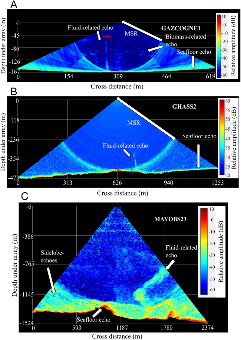
Figure 1. Geometry of the acoustic image of the water column from multibeam echosounder data (A) Kongsberg EM302 (GAZCOGNE1), (B) Seabat 7150 (GHASS2) and (C) Kongsberg EM122 (MAYOBS23). The sidelobe interference is visible as a circle arc with a radius equal to the Minimum Slant Range (MSR). These images correspond to the main acquisition configuration used for each survey (i.e., ‘shallow’ and ‘medium’ mode the GAZCOGNE1 and MAYOBS23 surveys, respectively).

MultiBeam EchoSounders (MBESs) record acoustic backscatter from targets located in the water column (e.g., Mayer et al., 2002). Each recorded ping cycle provides an image of the acoustic backscatter from the water column. MBESs are active sonars with two antennas, one for transmitting and one for receiving (Lurton and Augustin, 2010). These sounders are usually mounted on the ship hull and can have up to several hundred very narrow beams of the order of a degree (Table 1) (e.g., 288 and 880 beams for the EM302 and EM122 Kongsberg and the Reson 7150 MBES, respectively) distributed in the across-ship direction over an angular sector (swath). Thanks to their large swath (generally set between 120° and 170°), MBESs can cover a large area of the seabed (i.e., up to 5.5 times the water depth for an aperture of 140°) and a large volume in the water column. Since 2009, the use of acoustic water column data to detect fluids has been gaining momentum (Dupré et al., 2014; Sahling et al., 2014; Weber et al., 2014) but the amount of data recorded makes human interpretation very time-consuming. Moreover, discriminating fluid echoes from other natural echoes (e.g., fish shoals, acoustic artefacts associated with very backscattering seabed, noisy soundscapes) and MBES-related artefacts (e.g., beamforming, specular reflection) is a task that is currently mainly performed manually by specially trained experts. Therefore, human experts have to scrutinise Water Column Images (WCIs) ping by ping to detect a fluid emission. Various processing techniques (signal echo-integration, Dupré et al., 2014; Dupré et al., 2015; 3D dB threshold filtering; Schneider von Deimling et al., 2015) help the interpretation but are still of limited use, especially faced with large datasets. Also, this expertise must be updated when the sounder parameters or the sounder itself changes, and the time required for analysis limits its scalability and reproducibility.

Table 1

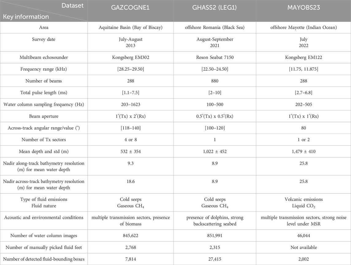
Table 1. Multibeam echosounder and acquisition parameters for the three investigated datasets with indications of the acoustic and environmental conditions. Tx and Rx refer to Transmission and Reception antennas, respectively. The number of water column images, manually picked fluid emission points and bounding boxes around detected fluids are indicated for each of the three studied datasets.

Few automatic detection methods have been implemented to address this issue. Urban et al. (2017) proposed using median filters in successive WCIs. Only one multibeam echosounder, the Kongsberg EM302, was used, with a frequency of 30 kHz, to survey an area in the North Sea, offshore Netherlands. The extraction threshold was set based on their survey. This method allowed for the identification of seep areas but was often hindered by side-lobe distortions and unwanted targets that can obscure or disrupt gas-plume information, resulting in a reduced analysis area in the water column. Therefore, only data from inside the minimum slant range can be processed with their method. The same multibeam echosounder, an EM302 from Kongsberg (30 kHz) was used by Weber (2021) for a survey in the Gulf of Mexico to locate gas seeps. Their Constant False Alarm Rate detector successfully removed 99.1% of the MBES raw data while preserving the targets of interest corresponding to 51 WCIs. Their method relies on the background noise being locally stationary in time, which is not always the case throughout the image. As a result, their method may underperform when there is a change in topography and/or seafloor substrate type.

The application of machine learning to water column images dedicated to the detection of emitted gas bubbles was first proposed by Zhao et al. (2020). Their method consists of a Haar-Local Binary Pattern cascade to combine information. Grey-level variations (e.g., edges, lines and center-surround features) are extracted by the Haar filters, while local texture information is provided by the Local Binary Pattern algorithm. A supervised Adaboost classifier is then learned based on these hand-crafted features. Their dataset was composed of a limited number of WCIs (1,444) acquired by a Kongsberg EM710 MBES (73–97 kHz transmission frequency) in the South China Sea. This method produced excellent results on their datasets with 95.8% accuracy. Nevertheless, it is worth noting that their database is characterized by its cleanliness, exhibiting minimal noise in the water column, which is not the case for most MBES surveys. This observation implies that their approach may not be fully tested to its limits.

There is a clear need to improve fluid detection as automatic methods developed so far (Urban et al., 2017; Weber, 2021; Zhao et al., 2020) are unreliable in the region under the top specular sidelobe in WCIs, i.e., below the so-called Minimum Slant Range (MSR) (Figure 1). Additionally, adapting to other WCIs from different multibeam sounders with varying acoustic configurations (e.g., frequency, aperture, and number of sectors), often changing during the same survey, has to be addressed. Exploring the potential of learning features and filters offers the prospect of greater sophistication, making the detection algorithm more finely adjustable and adaptable.

Deep learning algorithms, particularly convolutional neural networks, are increasingly being used for object detection in images due to their ability to learn features and classifiers from large datasets. A study on WCIs with hydrothermal fluid emissions using the You Only Look Once (YOLO) (version 5) algorithm (Jocher, 2021) was conducted by Mimura et al. (2023) who demonstrated the effectiveness of this algorithm in detecting hydrothermal fluids. The data were acquired during a survey conducted north of Okinawa Island (Japan) with a Kongsberg EM122 MBES (12 kHz). Their model achieved impressive results on the test set with a precision of 0.928, a recall of 0.881, and an F₁ score of 0.904. However, these positive results have to be moderated because of the limited number of images (280) in the test set and the fact that there are no other sources of acoustic echoes within the dataset (e.g., fishes, cetaceans).

The present study investigates the use of the YOLOv5 convolutional neural network for detecting fluids in water column images from MBESs. Our study aimed to find an adaptable and generalisable method to address this issue. To achieve this, MBES data from three marine expeditions were then used. The composition of the training dataset was analyzed under various conditions, including data acquired with several sounders (e.g., manufacturer, frequency), with additionally different acquisition settings (e.g., aperture, sector number), and diverse environmental conditions (e.g., noise level, biomass, fluid nature). The out-performance of our multi-MBES fluid detectors is discussed along with the most efficient way to reduce false positives. Recommendations on acquisition, processing and training set composition are given to successfully and rapidly detect emitted fluids in the water column from MBES data.

2 Materials and methods

2.1 Water column data from multibeam echosounder

A MBES sends an acoustic pulse from its transmit array towards the seafloor through the water column. The transmission geometry of the MBES enables coverage of a large area on the seafloor due to a wide emitted beam across-track and a good resolution capability due to a narrow-emitted beam along-track (Table 1). At reception, the MBES processes and digitizes the signal (amplification, filtering, base banding, sampling) on each element (transducer) before forming a series of directive beams covering a wide range of receiving angles, from starboard to port (Lurton et al., 2015). The digitized time series associated with each beam, displayed in polar geometry are the so-called Water Column Images (Figure 1). The MBES also includes algorithms for processing recorded raw data specifically for detecting the sea bottom, which is used as a reference to lower bound the WCI.

For the present study, we used data from three marine expeditions, the key facts of which are summarized in Table 1. The GAZCOGNE1 (Dupré et al., 2020; Loubrieu, 2013; Ruffine et al., 2017) expedition includes an exhaustive acoustic mapping of methane seeps in the Aquitaine Basin (Bay of Biscay). A 30 kHz Kongsberg EM302 MBES was operated (Figure 1A) and its acquisition parameters were modified during the survey according to the water depth change. The GHASS2 expedition (Riboulot et al., 2018; Riboulot et al., 2021) aimed at studying the dynamics of methane emissions, particularly their relationship with gas hydrates, sedimentary deformations, and submarine instabilities offshore Romania (Black Sea). A 24 kHz Reson Seabat 7150 was used (Figure 1B). The MAYOBS21 and MAYOBS23 expeditions (Feuillet et al., 2021; Rinnert et al., 2021; Jorry et al., 2022) surveyed the Fani Maoré volcano area, east of Mayotte Island, with a 12 kHz Kongsberg EM122 MBES (Figure 1C).

The first two datasets were labeled, i.e., an expert manually picked the foot of the fluid for at least one ping from the set of pings where the fluid is visible, and constitute our training datasets. These datasets were used to study the ability of our algorithm to learn to detect emitted fluids and to generalize to new data according to the composition of the training dataset. The most recent marine expedition, MAYOBS23, provided an opportunity to evaluate our algorithm operationally and was solely used for this purpose. Each dataset has different acoustic and environmental characteristics (Table 1), modifying slightly or deeply the perception of a fluid. This variability in characteristics is the reason why it is still difficult to learn a machine-learning detection model that can be used regardless of the sounders, their acquisition settings and the environmental conditions.

The acoustic characteristics concern both the specifications of each sounder and the acquisition parameters (Table 1). MBESs are different and have for instance a different operating frequency and beam aperture (Figure 2). Additionally, MBES acquisition parameters change during a mission. Kongsberg multibeam real-time software proposes to adjust EM302 acquisition parameters, including the number of transmission sectors, aperture angle and pulse length, according to water depth. The acoustic acquisition modes are classified as “deep” (Figure 2C), “medium” (Figure 2B), and “shallow” (Figures 1A, 2A), corresponding to 4, 7% and 89% of the GAZCOGNE1 dataset, respectively. It is worth noting that the EM302 MBES compensates for pitch and roll by creating steered emission sectors to optimize the geographical coverage (Tonchia and Parthiot, 1994). For instance, in deep mode, the EM302 utilizes up to eight sectors with slightly different frequencies, implying changes in sector transmit gains which can be observed in WCI (Figures 2A–C). During the GHASS2 expedition, the Seabat 7150 was operated in ‘auto’ mode, which resulted in significant and frequent changes in acoustic parameters throughout the entire survey (Figures 2D–F). In the MAYOBS23 dataset, obtained with an EM122 MBES, there are two acquisition modes, ‘shallow’ and “medium” corresponding to 5% and 95% (Figure 1C) of the dataset, respectively. As for the EM302, these two EM122 modes result in different pulse lengths, sampling frequencies and number of transmission sectors. However, these changes are limited for the MAYOBS23 dataset, due to the angular range reduced to 80° resulting in only two sectors in medium acquisition mode that represents the majority of this dataset (Figure 1C). It is worth noting that the antenna sidelobe levels were quite high for this survey. This resulted in very noisy WCIs below the Minimum Slant Range (Figure 1C). The MBES performs sea-bottom detection from raw data, which is then used as a reference to bound the WCIs. Failure to accurately detect the sea bottom may result in loss of information in WCIs as in the GHASS2 dataset (Figure 2E). This failure is not present in the GAZCOGNE1 and MAYOBS23 datasets. Additionally, for the GHASS2 dataset, WCIs may exhibit acoustic artefacts (under the minimum slant range) which can be confused with the signatures of fluids (Figure 2F). Regarding the environmental conditions, the biomass visible in the WCI is very dense in the GAZCOGNE1 dataset, due to the abundance of fishes in the Bay of Biscay (SIH, 2017; ICES, 2023) (Figure 2A). The presence of a high density of biomass may mask the fluids visible in the WCIs, as the texture of this biomass may be similar to that of the fluids. In contrast, in the GHASS2 dataset, little biomass is observed in the surveyed slope domain due to water anoxia in the Black Sea beyond 120 m below the sea level as observed during the GHASS2 marine expedition. There is no biomass clearly visible in the part of the studied MAYOBS23 dataset. Additionally, the GHASS2 dataset presents a challenge due to the presence of dolphins visually observed around the ship and for which typical echolocation signatures are displayed in WCIs (Figure 2E). Furthermore, the acoustic backscatter of the Black Sea seafloor is very high revealing a very reflective sea-bottom interface and causing artefacts at the nadir (Figure 2D).

Figure 2

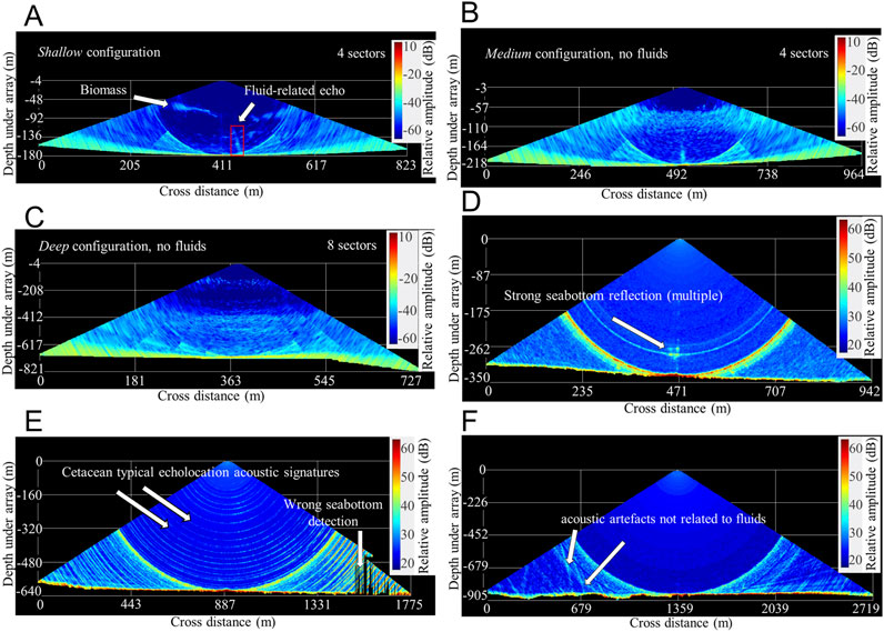
Figure 2. Geometry of water column images in the multibeam echosounder Kongsberg EM302 (GAZCOGNE1) (A,B and C) and Reson Seabat 7150 (GHASS2) (D–F) with different acquisition parameters. Frequency: (A) 29.5 kHz, (B) 29.25 kHz (C) 28.25 kHz, and (D–F) 22.5 kHz. Pulse length: (A) 1.125 m, (B) 3 m, (C) 7.5 m, (D) 2 m, (E) 3 m, and (F) 5 m. Angular range: (A, B) 140°, (C) 130°, and (D,E, F) 120°.

2.2 Deep learning-based object detection with YOLOv5

Deep learning algorithms are increasingly being used to detect objects in images, provided that labeled training datasets are available (Zou et al., 2023). This increasing attention is due to remarkable breakthroughs in supervised deep learning, particularly in object detection. Object detection is a computer vision task that is concerned with the detection and localization of objects of interest in digital images. This task requires extracting information to describe objects in an image at different scales and ratios, identifying regions of interest for these objects, and classifying them as either a known class or a background class. One of the challenges is to complete the task within a reasonable computational time. Two families of object detection algorithms were proposed in recent years (Zou et al., 2023). The first family uses a two-stage approach, where the regions that may contain an object are identified first, followed by object classification. Examples of this family include Faster R-CNN (Ren et al., 2015) and Mask R-CNN (He et al., 2018). The second family uses a single approach to solve both tasks simultaneously. Algorithms include YOLO (Redmon et al., 2015) and SSD (Liu et al., 2016). The two-stage algorithms are more accurate in detecting and localizing objects while one-stage algorithms have a better trade-off between performance and speed. It is worth noting that the performance of one-stage algorithms lowers noticeably when detecting dense and small objects.

In the present study, we investigated version five of the YOLO algorithm (YOLOv5, small (S) version) (Supplementary Text S1) developed by Ultralytics and released in June 2020 (Jocher, 2021) as we need a computationally efficient algorithm (Supplementary Text S2). The YOLO algorithm was one of the first algorithm to propose the one-stage approach, and many improvements were made leading to the fifth version. The architecture of YOLO is based on a feature extractor and a head dedicated to detection and localization. The feature extractor of YOLOv5, called CSPDarknet53 (Bochkovskiy et al., 2020), is based on a convolutional neural network which allows the spatial information contained in images to be hierarchically decomposed into features (LeCun et al., 2015; Goodfellow et al., 2016). Combining these multiscale features, the head is dedicated to answering the three following questions at three scales: Are there objects present in the image? If so, which class do they belong to? Where are these objects located in the image?

One of the peculiarities of a YOLO network is that it performs object detection in one step using anchor boxes (Supplementary Figure S1 given in the Supplemental Information). An image is divided into a grid of cells at three different scales. For each cell, three anchor boxes of different dimensions are considered as candidates for detecting an object at the scale and center of the cell (Supplementary Figure S1A). Thus, the trained detection model infers thousands of candidate bounding boxes (depending on image resolution and the number of anchors) from an input image (Supplementary Figure S1A). The model predicts the class of the object and locates it by predicting bounding boxes through offsets from the anchor boxes (Redmon et al., 2015). Candidate bounding boxes are retained if the probability of the presence of an object is significant. In our case, the threshold for inference is set to 0.3 (Supplementary Figure S1B). Finally, a non-max suppression algorithm (Neubeck and Van Gool, 2006) is applied because several bounding boxes for the same object may still be candidates (Supplementary Figure S1C).

2.3 Creation of the water column image datasets

This article presents a supervised machine learning approach that requires datasets associating WCIs and labels. Labels for object detection typically include the object’s class (i.e., fluid in our case) and bounding boxes.

For the acoustic data, we used Sonarscope software (Augustin, 2023) to convert MBES data stored in Kongsberg and Reson files to WCIs (Figure 3). For water column imaging, we applied a standard sonar correction as described in Urban (2017), during acquisition, using a Time-Varying Gain (TVG) defined as TVG = 30log10(R)+2⋅a⋅R + C, with R the range, a absorption coefficient in dB/m and C a constant gain. This correction accounts for propagation losses and is tailored for observing surface scattering at oblique angles, a regime where 30⋅log10(R) compensation is standard for multibeam echosounders (Lurton et al., 2015). A geometry transformation is then performed to convert the time-amplitude beam signals into polar spatial geometry (depth versus across distance representation of the amplitude). Finally, the WCIs are sea-bottom clipped based on the MBES bottom detection algorithm and digitized to 8 bits (Figure 3), a quantization level that at least matches the minimum quantification used for the water column data (8-bit in this case). The YOLOv5 (Jocher, 2021) model requires square images with dimensions of multiples of 32. This is achieved by resizing the longest side of non-square images (here the width) to the input size and padding with a grey background to maintain the aspect ratio. A width multiple of 32 was chosen, which is close to the average width for each dataset. The width represents 992, 960 and 760 pixels for GAZCOGNE1 GHASS2 and MAYOBS23, respectively.

Figure 3

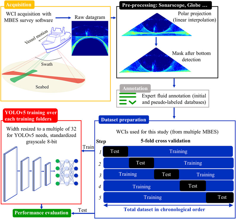
Figure 3. Methodology flowchart for water column records from multibeam acquisition to average performance evaluation. Raw datagram are pre-processed using for instance Sonarscope software to generate images used for expert fluid annotations. Then datasets for cross-validation are prepared in order to train and test YOLO performance.

The WCIs are labeled by an expert who visually identifies a fluid emission with GLOBE software (Poncelet et al., 2023), typically visible in a series of successive WCIs, and then pinpoints its foot on a single selected WCI. As a result of this protocol, only one WCI corresponding to the fluid emission point at the seafloor is labeled while the remaining WCIs are not labeled. Consequently, both datasets were manually re-labeled to match the labeling format for object detection, namely, a rectangular bounding box including the fluid instead of a point at the fluid foot.

Furthermore, each WCI underwent re-examination using detections made by a YOLOv5 model trained with expert foot points to identify fluid emissions. If a fluid emission was detected, a bounding box was assigned to the WCI, resulting in an increase in the number of annotated WCIs with a fluid label (Table 1). The GHASS2 cruise showed a significant increase in the number of bounding boxes compared to the expert points. This is mainly due to the high resolution of the Reson Seabat 7150 sounder and the numerous side lobes of the transmission antenna. Fluid-related echoes may appear in several consecutive pings, typically up to a maximum of 10, depending on vessel motion, backscattering intensity, and antenna used. The number of fluid feet for the MAYOBS23 is not given, but bounding box labeling was carried out, resulting in 2,002 bounding boxes among 46,044 WCIs.

2.4 Training and evaluating the YOLOv5 model

Training an object detection model is a complex process that usually requires a large labeled dataset as the model has 7.2 million parameters. Transfer learning can be used when only a small amount of data is available for training (Pan and Yang, 2010). Transfer learning is the idea of reusing the previously learned algorithm from other tasks. In the case of YOLOv5, the base weights of a network already trained on the Common Objects in COntext (COCO) dataset (80 optical classes) (Lin et al., 2014) are provided by the YOLOv5 authors (Jocher, 2021). It is possible to retrain a part of this network with other data (e.g., images with fluid-related echoes). This allows the network to reuse certain common features between the old classes and the new ones, for more efficient training.

For the training phase of YOLOv5, the expression of the loss function (which measures the errors made by the network compared to the ground truth) is composed of three weighted terms (Equation 1): i) class loss L_cls (high value if it is not the correct object class in the box predicted by YOLOv5), ii) objectness loss L_obj (high value if there is no object in the box), and iii) box loss L_box (high value if the box is not where the actual box is).

$Loss={\lambda }_1{L}_{cls}+{\lambda }_2{L}_{obj}+{\lambda }_3{L}_{box}(1)$

The first two terms are computed using a cross-entropy loss, which measures the closeness between the distributions of the truth and the predictions. The last one is calculated using a complete intersection over union loss which measures the difference in overlap, ratio, and distance between the predicted boxes and the true boxes.

The main hyperparameters are given in the Supplemental Information (Supplementary Table S1) (Freund and Schapire, 1995; Jocher, 2021). The maximum number of epochs for YOLOv5 is fixed at 50. Early stopping is employed when there is no improvement on the validation data after 10 consecutive epochs, leading to the cessation of training.

Evaluating a model necessitates at least two datasets. A training set allows assessment of the capacity to learn from data, and a testing set evaluates the ability to generalize to data not seen during the training. Our tests were carried out under a cross-validation scheme. Cross-validation is used to assess model performance, prevent overfitting, and maximize data use (especially important when data including target of interest is scarce) (Figure 3). To limit computational time, only five folds (subsets) were defined from both GAZCOGNE1 and GHASS2 WCI datasets (Supplementary Table S2). Data were not shuffled. We maintained the chronological order of acquisition to avoid data leakage (Yagis et al., 2021), and we tried to balance the number of fluids in each fold. As a result, each fold contains an average number of 169,124 WCIs (1 563 fluid bounding boxes) for GAZCOGNE1 and 126,323 WCIs (5,483 fluid bounding boxes) for GHASS2 (Tables 1; Supplementary Table S2). MAYOBS23 was solely used for inference so no cross-validation was performed on this dataset.

There are four possible cases when we compare object detection predictions with ground truths, through the so-called confusion matrix (Figure 4). A detection is considered to be a True Positive (TP) if an expert identified a fluid foot (a point in the WCI) that lies between the minimum x coordinate and the maximum x coordinate of the predicted box by the YOLOv5 learned model. If not, the detection corresponds to a False Positive (FP). Undetected echoes may either concerns actual fluid-related echoes (False Negative, FN) or unwanted targets (True Negative, TN). We used classical features computed from the confusion matrix: accuracy (Equation 2), precision (Equation 3), recall (Equation 4), and Matthew’s Correlation Coefficient (MCC) (Equation 5) with True Positives (TPs), True Negatives (TNs), False Positives (FPs); False Negatives (FNs).

$accuracy=\frac{TPs+TNs}{TPs+TNs+FPs+FNs}(2)$

$precision=\frac{TPs}{TPs+FPs}(3)$

$recall=\frac{TPs}{TPs+FNs}(4)$

$MCC=\frac{TNs*TPs-FPs*FNs}{\sqrt{\left(TNs+FNs\right)\left(FPs+TPs\right)\left(TNs+FPs\right)\left(FNs+TPs\right)}}(5)$

Figure 4

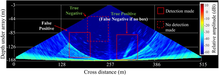
Figure 4. Examples of True Positive (TP), True Negative (TN), False Positive (FP), and False Negative (FN) water column detections from GAZCOGNE1 data.

Accuracy corresponds to the rate of correct predictions. Precision indicates the proportion of true positives made by the algorithm among all positive predictions. The higher the precision, the fewer false positives. Recall indicates the proportion of actual positives correctly identified by the algorithm. The higher the recall, the fewer false negatives. In the case of unbalanced data sets, the MCC is a more reliable statistical indicator than the accuracy (Chicco et al., 2021) because it gives equal weight to each class. For example, if a dataset contains many images without fluid (and only few images with fluid) and the networks detect nothing, it would have a high accuracy (because of many true negatives) but a low MCC (which is more representative of the network performance).

Finally, it is worth noting that we did not evaluate the accuracy of the localization of the predicted bounding boxes since the expert annotation is a fluid foot point. In the present study, we only focus on detection performance.

2.5 Training, evaluating and optimizing a YOLOv5 model

In deep learning, training an efficient model means composing a dataset, defining the network architecture and choosing hyperparameters of the model, the cost function used to learn a task and the optimizer in charge of solving the problem. While choices are classical for object detection, the present study focuses on the composition of the dataset and its influence on the performance of detection. Datasets must be representative of the variability of the data world. As previously mentioned, the world of WCIs is based on sounder parameters and processing, environmental conditions, soundscapes and geographic areas. In this study, three datasets were used; created from a long effort made by geoscience experts to label WCIs. The resulting datasets are very precious, but not ready to use for learning an accurate model. The datasets suffer from imprecision due to the annotation process, as only one fluid foot is pointed within a row of several pings where the same fluid is observable. These three datasets are an interesting playground to analyze the way to optimize the training process to increase the performance of fluid detection and obtain a fluid detection model which can be used for different sounders. The composition of the training and testing sets for each of the seven conducted experiments (Figure 5) is detailed in the following paragraphs. Before training and inference, all input data were normalized, effectively mitigating relative amplitude differences between sonar types (Kongsberg and Reson). Neural networks perform better when input data are normalized as this stabilizes computations within the network layers, reduces unstable gradients, and accelerates the convergence of the learning process.

Figure 5

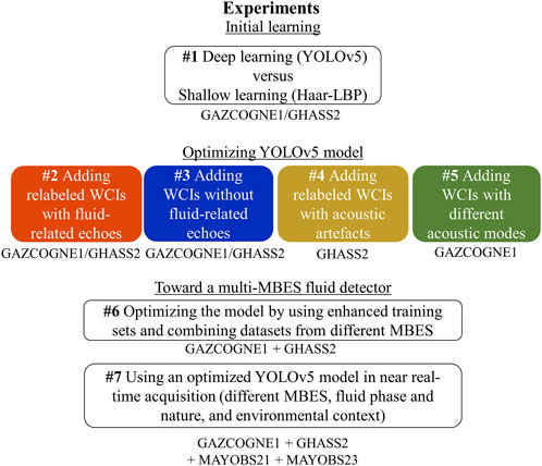
Figure 5. Experiments used for the assessments, according to the composition of the training set. LBP, WCI, MBES stand for Local Binary Pattern, Water Column Image and MultiBeam EchoSounder, respectively.

Before all, we studied the efficiency of the YOLOv5 model as a deep learning approach to surpass the traditional machine learning approach (Experiment #1 in Figure 5). We implemented the handcrafted features and classifier used by Zhao et al. (2020) based on the information provided in their article. As previously mentioned, we trained and evaluated the YOLOv5 model with the five-fold cross-validation procedure separately for GAZCOGNE1 and GHASS2 (Supplementary Table S2). To fairly compare both approaches, we adopted the same balance used by Zhao et al. (2020) between WCIs with and without fluid in the testing set. The resulting testing set has thus 70% WCIs with fluid and 30% without (Table 2).

Table 2

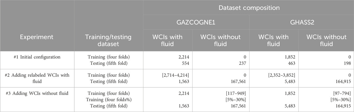
Table 2. Examples of the compositions of the training datasets and the datasets used for testing (inference) for Experiment #1 (initial configuration training), Experiment #2 with addition of relabeled water column images with fluid-related echoes, and Experiment #3 with addition of water column images without fluid-related echoes. An example of a cross-validation dataset (one fold) is given each time, representing the mean configuration used. WCI stands for Water Column Image.

Then we strove to optimize the YOLO training dataset composition in four ways (Experiments #2 to 5, Figure 5). The second experiment (#2) concerns the addition of re-labeled WCIs containing fluid. The initial datasets were useful for obtaining the first detection models. To optimize the annotation process, models learned in the first experiment served to pseudo-label respective datasets. Not all fluid emissions were indeed annotated in the first datasets because experts only pointed the fluid outlet. For example, if an echo from the same fluid emission is seen in 10 successive pings, it is only pointed once at the assumed outlet. To find other fluid labels, a neural network trained with the initial configuration set on all GHASS2 and GAZCOGNE1 pings (Table 1) was used to enrich our annotated database. This method called pseudo-labeling (Lee, 2013; Wu and Prasad, 2017; Stanchev et al., 2020) is a simple and efficient solution that allows for labeling large unlabeled datasets with a network trained with a little labeled dataset. A similar CNN-assisted annotation method was successfully proposed for underwater optical images (Zurowietz et al., 2018). The detections we obtained were then manually classified into False and True Positives before adding them to our training sets to prevent any incorrectly labeled WCIs from being included in the training set. Good detections (WCIs with “fluid” labels) were thus added to the previously “fluid” class (Table 2). Ambiguous cases, such as echoes for which it was unclear whether they represent fish or fluid (e.g., GAZCOGNE1 cruise), were omitted to avoid introducing incorrect information into the neural network training. Consequently, only unambiguous cases were included in the training datasets to ensure data quality and model reliability. The GAZCOGNE1 campaign having a limited number of fluid-related echoes, we decided to add a maximum of 2,000 fluid labels in 500 steps. We followed the same methodology for GHASS2.

To ensure a fair comparison of the results, experiments #2, 3, 4 and 6 use the testing set from the entire validation folds of the concerned cruise(s), including WCIs with and without fluid (Tables 2–4).

Table 3

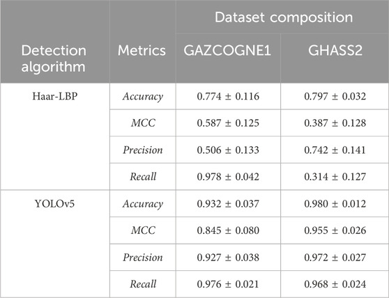
Table 3. Performance metrics on GHASS2 and GAZCOGNE1 data sets with Haar Local Binary Pattern and YOLOv5 (Experiment #1). MCC stands for Matthews Correlation Coefficient.

Table 4

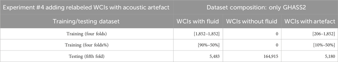
Table 4. Examples of the compositions of the training datasets and the datasets used for testing (inference) for Experiment #4 dedicated to the Seabat Reson 7150 acoustic artefacts. An example of a cross-validation dataset (one fold) is given each time, representing the mean configuration used. WCI stands for Water Column Image.

We conducted a third experiment (#3) by adding WCIs without fluid to the model. Our datasets contain a large number of files without any fluid corresponding to 56% and 55% of the total WCIs for GAZCOGNE1 and GHASS2, respectively (Table 2). We investigated the adding value of increasing the number of WCIs without fluid. Adding “background” WCIs could help the model to learn either artefacts caused by the characteristics of the MBES and other acoustic systems and echoes related to the environmental conditions (e.g., fish shoals). WCIs without fluid could thus show the network negative samples that the network must not detect and therefore the network could successfully manage scenarios with a lot of noise. In the present study, the number of WCIs without fluid varies in the training set for each fold, from 5% to 30% of the total number of WCIs (Table 2).

A fourth performance study (Experiment #4) was then carried out following the large number of acoustic artefacts detected as fluids by the initial model for the GHASS2 dataset (used in Experiments #1–3) (Supplementary Figure S2). These WCIs were subsequently relabeled in a second class “acoustic artefacts/environmental phenomena” and integrated into our training sets (Table 4). Consequently, a database of 22,377 second-class labels was created. This technique is known as hard negative mining and enables the network to concentrate on identifying non-fluid objects (Parkhi et al., 2015; Schroff et al., 2015; Shrivastava et al., 2016). To determine the percentage balance between the two classes, “fluids” and “acoustic artefacts/environmental phenomena”, we created training sets that contain a maximum of 50% of “acoustic artefacts/environmental phenomena” labels. Hard negative mining was not relevant to be conducted for the GAZCOGNE1 dataset because of the too limited numbers of “acoustic artefacts/environmental phenomena” labels. In numerous WCIs, it is indeed impossible to distinguish with certitude biomass-related echoes from fluid-related echoes due to their spatial overlay.

A fifth experiment (Experiment #5) was conducted to explore the possible influence of the different acquisition modes from the Kongsberg EM302 multibeam echosounder (Figures 2A–C; Table 5). Four combinations of acquisition modes were thus used in training sets, with WCIs acquired in i) shallow, ii) shallow and medium, iii) shallow and deep and iv) shallow, medium and deep modes. We did not explore other configurations (e.g., deep and medium or medium) because there were not enough fluid points in these configurations to train the network. Within the fluids manually pointed by the experts, there are 2,730 in shallow mode, 38 in medium mode and 0 in deep mode. For GHASS2, as there are too many acquisition parameter combinations, effects of acoustic modes on model performance were not explored.

Table 5

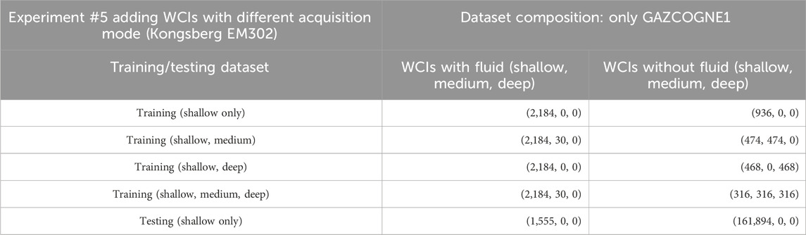
Table 5. Examples of the compositions of the training datasets and the datasets used for testing (inference) for Experiment #5 relative to the Kongsberg EM302 acquisition modes. An example of a cross-validation dataset (one fold) is given each time, representing the mean configuration used. WCI stands for Water Column Image.

We finally implemented a strategy to learn a general model usable for different sounders (Kongsberg EM302 and EM122, Reson Seabat 7150), different locations (Atlantic Ocean, Indian Ocean, Black Sea), and different nature and phase of fluid (gaseous methane and liquid carbon dioxide) (Table 1). The strategies (#1–5) were thus combined to obtain an optimized model with enhanced training set (Table 6) used subsequently for experiment #6. First, to evaluate the complementarity of different sounders and geographical areas but with the same emitted fluid (i.e., gaseous methane), we explored the possibility of learning from GAZCOGNE1 and applying to GHASS2 and vice versa and the possibility of learning from both (Experiment #6). To complement the study, the MAYOBS23 dataset was investigated in near-real time of acquisition with another MBES (i.e., Kongsberg EM122), another nature of fluid (i.e., liquid CO₂ instead of gaseous CH₄) and another location and environmental context (Experiment #7).

Table 6

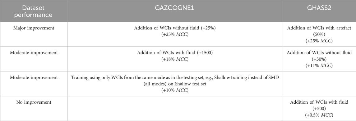
Table 6. Maximum YOLOv5 performance depending on training set composition (Experiments #2–5) for both GAZCOGNE1 and GHASS2 datasets. WCI and MCC stand for Water Column Image and Matthews Correlation Coefficient, respectively.

3 Results

3.1 Initial learning with experiment #1: Deep learning (YOLOv5) versus shallow learning (Haar-LBP)

The first experiment consists of comparing the performance of a traditional shallow learning method with a YOLOv5 model by reproducing the method from Zhao et al. (2020) on both GAZCOGNE1 and GHASS2 datasets. Details on training and testing sets are exposed in Table 2 with performances of both Haar-LBP and YOLOv5 using a five-fold cross-validation reported in Table 3. The results are presented as a mean and a margin of error at a 95% confidence level.

As the data sets are unbalanced with 70% WCIs with fluid and 30% without fluid to fit with Zhao et al. (2020), MCC is a more reliable metric for result analysis than accuracy. For instance, the GHASS2 Haar-BLP inference reaches a relatively high accuracy of 0.797 but the MCC is only 0.387 indicating low recall (0.314) and high precision (0.742) (Table 3).

Performance of the Haar-LBP method varies significantly between the two datasets. For example, Haar-LBP achieves an average MCC of 0.587 for GAZCOGNE1 and a lower value of 0.387 for GHASS2. The margins of error of the performance metrics for both datasets are large, mainly over 0.1, indicating a high degree of dispersion between the cross-validation folds. For the GHASS2 dataset, precision of Haar-LBP is much higher (0.742) than recall (0.314), which suggests a notable number of undetected actual fluids. In contrast, the GAZCOGNE1 model results in a precision of 0.506 and an elevated recall of 0.978 which indicates a high number of false fluid detections.

YOLOv5 demonstrated a stronger performance on both datasets than the Haar-LBP model, suggesting its proficiency in extracting and utilizing features for fluid detection and location. The different metrics, including MCC, range from 0.845 to 0.980 (Table 3). The high precision and recall values for YOLOv5 (0.927–0.976) suggest a low number of false detections and a high number of good detections for both datasets. The performance of the GHASS2 dataset surpasses even the GAZCOGNE1 dataset with a significantly higher MCC of 0.955 compared to 0.845. The margins of error at a 95% level of the MCC of GAZCOGNE1 are three to four times larger than those of GHASS2 for an equivalent volume of data. Therefore, a model trained on the GAZCOGNE1 dataset is slightly less stable than a model trained on GHASS2. Examples of detections achieved using neural networks trained in this experiment are available in Supplementary Videos S1, S3. It is noteworthy that the neural network demonstrates the capacity to detect non sub-vertical fluid-related echoes caused by current (Supplementary Figure S3).

3.2 Optimizing YOLOv5 deep learning model

3.2.1 Experiment #2: Adding relabeled WCIs with fluid-related echoes

The initial trained model (Experiment #1) was then used on all datasets and allows fluid detection labels increasing to 7,814 and 27,415 the number of fluid labels for GAZCOGNE1 and GHASS2 dataset, respectively (Table 1). The second experiment aims to evaluate the effect of including these new true positive detections as relabeled WCIs in the training set on the performance of YOLOv5. The composition of the training set consists of WCIs from four out of five possible folds, with a maximum of 2,000 WCIs with fluid added in training sets (Table 2). The test set corresponds to the fifth fold. The performance metrics are plotted against the number of added WCIs with fluid-related echoes (Figures 6A,B).

Figure 6

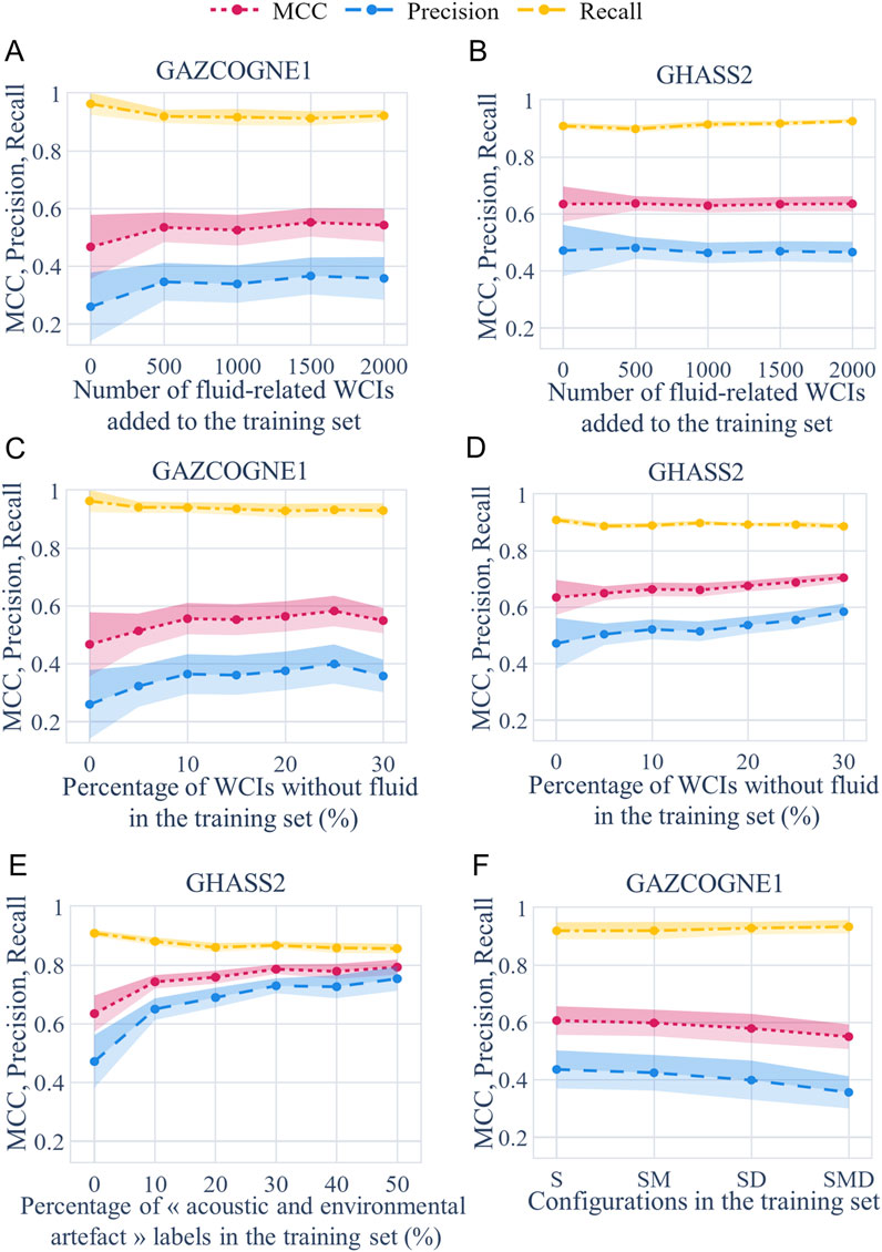
Figure 6. Performance metrics and their margin of error at a 95% confidence level as a function of the number of Water Column Images (WCIs) with fluid added in the training set (Experiment #2) (A) GAZCOGNE1, (B) GHASS2; the percentage of WCIs without fluid-related echoes in the training set (Experiment #3), (C) GAZCOGNE1, (D) GHASS2; (E) the percentage of “acoustic and environmental artefact” labels added to the training set (Experiment #4); and (F) acquisition mode configurations used in the training set (Experiment #5) based on WCIs acquired in shallow mode (GAZCOGNE1). Shallow (S), Shallow-Medium (SM), Shallow-Deep (SD), Shallow-Medium-Deep (SMD). MCC stands for Matthews Correlation Coefficient.

Whereas recall is high with a significant value of 0.9 almost constant whether or not WCIs with fluid are added, other performance metrics (MCC and precision) differ in value and trend between the two studied datasets. For GAZCOGNE1, we observe a +18% maximum increase in MCC from 0.468 (no WCIs with fluid) to 0.553 (1500 added WCIs with fluid) (Figures 6A,B). However, after the addition of only 500 WCIs, the MCC already reaches a value of 0.536, plateauing at around 0.54. Moreover, precision for GAZCOGNE1 significantly improves with the addition of only 500 WCIs with fluid (from 0.260 to 0.346 or +33%). This indicates a decrease in false positives as more information is provided to YOLOv5, from 14,164 to 7,634 or −46%. The percentage of images with detection (FPs + TPs) shows a steep decrease of 37.7% from 11.2% to 7.0%. Meanwhile, the MCC for GHASS2 remains stable whether or not images with fluid are added to the training set (from 0.635 to, e.g., 0.638 with 500 added WCIs with fluid). Other metrics for GHASS2 follow the same trend and remain unchanged while increasing the number of added WCIs with fluid (e.g., precision around 0.5).

Additionally, the performance of the network on the GAZCOGNE1 dataset is dependent on the amount of biomass present in the inference data fold. As each fold may not contain the same amount of biomass, which can be falsely detected as a positive by the network, there is some variability in the number of false positives. Therefore, the margins of error of precision and MCC metrics are larger for GAZCOGNE1 than for GHASS2. The margin of error for precision with 500 added WCIs with fluid reaches 0.131 and 0.077, respectively (Figures 6A,B). In particular, when there is a significant amount of biomass (e.g., GAZCOGNE1 part 4, Supplementary Table S2), there is a noteworthy improvement for MCC and FPs. MCC increases by 49% (0.348 and 0.517 for 0 and 2 000 added WCIs with fluid, respectively) and FPs strongly decrease by 63% (from 11,712 to 4,290 for 0 and 2 000 added WCIs with fluid, respectively). However, when the water column contains significantly less biomass (e.g., GAZCOGNE1 part 2, Supplementary Table S2), the MCC only increases by 18.5% (from 0.676 to 0.801 for 0 and 2,000 added WCIs with fluid, respectively) and FPs decrease from 4,293 to 1,507 (−65%) for 0 and 2,000 added WCIs with fluid, respectively.

It is important to note that despite higher MCC values for Experiment #1 than for Experiment #2, the first experiment does not outperform the second experiment. The evaluation protocol of Experiment #1 is indeed based on a testing set with 70% of WCIs with fluid and 30% without fluid to be able to fairly compare our results with those of Zhao et al. (2020), resulting in fewer false positives. In contrast, the second experiment adopted the natural dataset distribution: ∼0.1% with fluid and ∼99.9% without fluid for GAZCOGNE1 (∼5% vs. ∼95% for GHASS2). The change in the testing dataset protocol results in false positives due to the high number of WCIs without fluid as demonstrated by the precision curve of both datasets (Figures 6A,B).

In summary, the inclusion of WCIs with fluid has a varying effect on both datasets. While the GHASS2 dataset does not show an improvement, the addition of only 500 WCIs with fluid leads to an improvement in the performance of GAZCOGNE1; performances are enhanced for datasets containing copious biomass.

3.2.2 Experiment #3: Adding WCIs without fluid-related echoes

The objective of this third experiment is to evaluate the influence of adding WCIs without fluid-related echoes to the training set on network performance. It is important to note that the training dataset for this third experiment does not include the relabeled WCIs with fluid-related echoes used in experiment #2 (Table 2). Furthermore, the number of WCIs without fluid-related echoes is gradually combined with WCIs that have fluid-related echoes, starting from 5% of the entire training set and increasing up to 30%.

For both datasets, adding WCIs without fluid effectively increases MCC (Figures 6C,D). This has a greater effect on improving MCC for GAZCOGNE1 compared to GHASS2. Specifically, adding 25% of WCIs without fluid (i.e., 738) to the training set results in a maximum increase in MCC for GAZCOGNE1 by 25%, from 0.468 to 0.583. Similarly, adding 30% of WCIs without fluid (i.e., 794) to the GHASS2 training set leads to an 11% increase in MCC, from 0.635 to the maximum reached value of 0.705. For both datasets, this MCC improvement is mainly due to an increase in precision and is moderated by a slight decrease in recall (Figures 6C,D). For GAZCOGNE1, precision rises by +54% from 0.260 (no added WCIs without fluid) to 0.400 (25% of added WCIs without fluid) with recall decreasing by −3% from 0.965 to 0.934. For GHASS2, precision rises from 0.472 (no added WCIs without fluid) to 0.585 (30% added WCIs without fluid) (+24%) and recall slightly decreases from 0.910 to 0.887 (−3%). Detections of actual fluid for the initial model (no WCIs without fluid) are 3,921 and 5,322 for GAZCOGNE1 and GHASS2 datasets, respectively. TPs are more or less stable along with the addition of WCIs without fluid, with minor variations for both datasets (e.g., −5.5% with 25% of added WCIs without fluid for GAZCOGNE1 and -1.1% with 30% of added WCIs without fluid for GHASS2).

The results indicate a notable decrease in FPs for both datasets, by −57% for GAZCOGNE1 (from 14,164 to 6,033 for 0% and 25% of added WCIs without fluid, respectively) and by −39% for GHASS2 (from 6,315 to 3,870 for 0% and 30% of added WCIs without fluid, respectively). Adding WCIs without fluid can be particularly relevant in areas highly populated by biomass (e.g., GAZCOGNE1) because it enhances the performance (e.g., MCC) of the model. MCC improvement is more significant for a dataset with significant amounts of biomass (e.g., GAZCOGNE1 part 4, Supplementary Table S2) than for a dataset with considerably less biomass (e.g., GAZCOGNE1 part 2, Supplementary Table S2). MCC increases for GAZCOGNE1 part 4 by 47% (from 0.348 to 0.510 for 0% and 25% of added WCIs without fluid, respectively), but only by 17% for GAZCOGNE1 part 2 (from 0.677 to 0.793 for 0% and 25% of added WCIs without fluid, respectively). The variability in MCC increase between the two parts and the similar FPs reduction for both parts (−55%) indicate that FNs increase less in part 4 (+161%) where there is a significant amount of biomass, than in part 2 (+242%) characterized by much less biomass. There is a variability in FPs decrease among the different GHASS2 folds, with, e.g., a 46% reduction for the first validation fold and a 19% reduction for the second validation fold. However, it would be too complex to provide a comprehensive explanation for GHASS2, given the inherent variability in the Reson 7150 acoustic configurations and the different imbalances between the validation folds.

Adding WCIs without fluid-related echoes (+25 and +30% for GAZCOGNE1 and GHASS2, respectively) results in an increase in undetected actual fluids (FNs) by 105% for GAZCOGNE 1 (from 146 to 299) and by 24% for GHASS2 (from 530 to 655).

3.2.3 Experiment #4: Adding relabeled WCIs with acoustic artefact

The fourth experiment aims to evaluate the consequence of adding WCIs labeled as “acoustic and environmental artefact” labels to the training set on YOLOv5 performance to detect fluid. In addition to WCIs with fluid and WCIs without fluid, a third class (or second “labeled class”) “WCIs with artefacts” is introduced into the training data set. Table 4 provides the distribution of GHASS2 WCIs in the training set (fours fold) and the testing set (one-fold).

The addition of “acoustic and environmental artifact” labels leads to a significant increase in MCC from 0.635 (0%) to 0.794 (50% or equal number of labels for ‘fluid’ and ‘artefact’ class) (+25%) (Figure 6E). The precision clearly shows the same trend with an increase of 60% (from 0.472 to 0.755 for 0% and 50% of added WCIs with artefacts, respectively) indicating a substantial decrease in FPs. The decrease in false positives is particularly noteworthy, with a reduction of 74% from 6,315 to 1,638 (for 0% and 50% of added WCIs with artefacts, respectively) while the true positives are relatively stable with a minor decrease of 8% (from 5,322 to 4,889 for 0% and 50% of added WCIs with artefacts, respectively).

As the percentage of WCIs with artefacts increases, recall decreases slightly by 6% from 0.910 to 0.857 (for 0% and 50% of added WCIs with artefacts, respectively) indicating a loss in detection of actual fluids. These false negatives increase by 49% from 530 to 792 (for 0% and 50% of added WCIs with artefacts, respectively). This is however negligible compared to the number of detected-fluid bounding boxes which is 27,415 (i.e., 5,483 on average in each of the five folds) (Table 1).

Adding an extra class of acoustic artefacts clearly improves YOLOv5’s ability to differentiate between fluids and artefacts. This is the most effective method for the GHASS2 dataset to reduce detections and in particular false positives, despite a slight increase in undetected actual fluids.

3.2.4 Experiment #5: adding WCIs with different acquisition modes

The fifth experiment aimed to assess the effect on network performance when not all EM302 sonar acquisition configurations (deep, medium, shallow) are provided to the network. For this purpose, different acoustic modes (i.e., corresponding to varying frequencies, apertures, and numbers of sectors, Figures 2A–C; Table 1) were combined in the same training set (Table 5). The training set is thus composed of i) WCIs with fluid in Shallow and/or Medium modes and ii) WCIs without fluid in Shallow and/or Medium and/or Deep modes (corresponding to 30% of WCIs). One testing set with only WCIs in shallow mode was used (Table 5). Testing sets using medium and deep modes were not used as there are only a few fluid-related echoes and none in both of these modes, respectively.

Training using only WCIs from the same mode as in the testing set; e.g., in our case from the shallow mode (instead of combining all modes, i.e., SMD); provides the best results with a MCC increase of 10% (from 0.551 to 0.608). The addition of combined WCIs from different acquisition modes (S Shallow; SM Shallow and Medium; SD Shallow and Deep and SMD Shallow, Medium and Deep) in the training set leads to a gradual decrease in MCC from S, SM, SD and to SMD combinations with −9% from 0.608 (S) to 0.551 (SMD) (Figure 6F). Similarly, precision decreases from S, SM to SD combinations with the worst performance for the SMD combination with an overall decrease of −18% from 0.437 (S) to 0.357 (SMD) (Figure 6F). Recall is stable with low variations (+0.1–1.6%) from 0.920 (S), 0.921 (SM), 0.930 (SD) to 0.935 (SMD). The greater the difference in acoustic configuration (e.g., four transmission sectors in shallow and medium mode versus eight in deep mode), the more significant the decrease in MCC and precision. The data show an increase in false positives by + 25% from 5,076 with S training to 6,338 with SMD training and a minor decrease in false negatives by −8% from 305 with S training to 281 with SMD training. Larger differences in acquisition configuration leads to more significant decreases in false negatives and increases in false positives.

Adding WCIs in the training set from acquisition modes that are different from the one characterizing the testing set affects YOLOv5’s ability to extract reliable information on fluid in a contrasted way: i) negatively by increasing FPs and ii) positively by reducing the number of undetected actual fluid (FNs).

3.2.5 YOLOv5-model performance from varying training set composition

In previous experiments (#2–5), we employed various strategies to enhance the model’s performance by modifying the training set composition (for each of the two cruises separately) (Table 6). The addition of WCIs without fluid-related echoes helped to decrease false positives during inference for both datasets (Experiment #3). Furthermore, including examples of echoes that should not be detected (namely, acoustic and environmental artefacts) in a separate class reduces furthermore the number of false positives (Experiment #4 for GHASS2 dataset). Inclusion of additional WCIs with fluid can either enhance network performance, with a plateau being reached fairly quickly with only 500 additional WCIs (GAZCOGNE1 dataset case, Experiment #2) or have no effect at all (GHASS2 dataset case, Experiment #2). Additionally, providing all examples of the sounder’s acquisition configuration for Kongsberg MBES (the case of the EM302, GAZCOGNE1 dataset, Experiment #5) can increase the number of false detections when actual fluids are predominantly located in water depth ranges surveyed with a single acquisition mode. It is crucial to note that the most effective strategy for one dataset may not be effective for another. For instance, the addition of artefact labels and the inclusion of WCIs without fluid are the most effective in terms of MCC enhancement for GHASS2 and GAZCOGNE1, respectively (Table 6).

3.3 Towards a multi-MBES fluid detector

3.3.1 Experiment #6: optimizing the model by using enhanced training sets and combining datasets from different MBES

3.3.1.1 Enhanced training sets (same campaign)

The sixth experiment evaluates the effectiveness of a model trained with data either from a single campaign (GAZCOGNE1 or GHASS2) or from both campaigns (Table 7) with acquisition conducted with two different MBES (Kongsberg EM202 and Reson Seabat 7150, Table 1). To achieve this, we first selected the best YOLOv5 MCC performance training datasets for GHASS2 and GAZCOGNE1 from previous experiments (#2–4) with regard to the number of added WCIs with fluid, percentage of added WCIs without fluid, and the percentage of added WCIs with acoustic and environmental artefacts (Table 6). Then, we combined these enhanced training sets (Table 7). The evaluation is made whether the testing set contains WCIs for GAZCOGNE1 or GHASS2.

Table 7

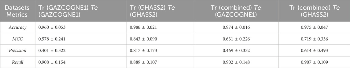
Table 7. Performance metrics and their margins of error at a 95% confidence level for Experiment #6 conducted with enhanced and combined training sets. Tr, Te and MCC stand for Training, Testing, and Matthews Correlation Coefficient, respectively. For example, Tr (combined) Te (GHASS2) refers to a model trained on both GAZCOGNE1 and GHASS2 data and tested only on GHASS2 data.

3.3.1.2 Combining datasets from different MBES

When examining the performance of the network trained with both marine expedition data (Tr (combined), Table 7, last two columns), we obtained contrasting results for both datasets. GAZCOGNE1 model demonstrates slightly better performance with an increase of 9% in MCC (from 0.578 to 0.631) and 17% in precision (0.469 versus 0.401) indicating less false detections while recall remains stable (0.902). In contrast, the addition of GAZCOGNE1 WCIs to the GHASS2 training set results in a decrease in GHASS2’s performance, by −15% for MCC (from 0.843 to 0.719) and by −25% for precision (from 0.817 to 0.614). However, recall slightly increases from 0.889 to 0.907 (+2%).

3.3.2 Experiment #7: evaluating an optimized YOLOv5 model in near real-time acquisition

During the MAYOBS23 monitoring mission (Jorry et al., 2022), we operationally tested an optimized YOLOv5 model for real-time fluid detection. The challenge was fourfold: i) the network had not yet been trained on the WCIs produced by Kongsberg EM122 MBES (Table 1), ii) the nature and phase of the emitted fluids were different from those studied during the GHASS2 and GAZCOGNE1 marine expeditions (liquid carbon dioxide versus gaseous methane), iii) the environmental acquisition conditions were different, and iv) the model had not yet been deployed in near real-time acquisition during a marine expedition.

Two different training configurations (Table 8) were used based on results from Experiment #6 (Table 7, last two columns). The first training set in Table 8 combines two previously studied GAZCOGNE1 and GHASS2 data sets (Table 7). The second training set includes in addition WCIs acquired in identical conditions (vessel, MBES) during a past marine expedition in the same area (MAYOBS21, Rinnert et al., 2021). The MAYOBS21 training set concerns 1,384 Kongsberg EM122 WCIs corresponding to 1,176 WCIs with fluid and 208 without fluid. The MAYOBS23 testing set consists of 1,468 WCIs with fluid and 46,044 without.

Table 8

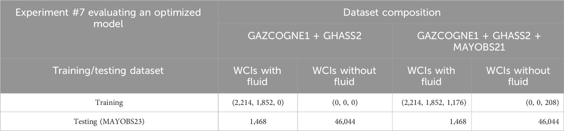
Table 8. Composition of the training and testing datasets used for the near-real time acquisition mission MAYOBS23 (Experiment #7). For the training set, values are given in the following format (Number of WCIs from GAZCOGNE1, GHASS2, and MAYOBS21 dataset). WCI stands for Water Column Image.

The model trained, including MAYOBS21 data, performed better than the model only trained with GAZCOGNE1 and GHASS2 (Table 9). While accuracy and recall for both models have relatively the same level (from 0.973 to 0.986 or +1% and from 0.850 to 0.826 or −3%, respectively), MCC and precision significantly increase. MCC increases by +14%, (from 0.698 to 0.797) and precision by +32% (from 0.595 to 0.783). These results suggest that both models have a similar number of FNs whereas adding MAYOBS21 data to the second training set drastically reduced FPs. Specifically, 85% and 83% of actual fluid-related echoes were detected with both models, with 262 and 287 undetected fluid-related echoes for the first and second training sets including MAYOBS21 data, respectively. There were 1,011 FPs for the first model and only 377 (a decrease of 63%) for the second training set (GAZCOGNE1, GHASS2 and MAYOBS21 data).

Table 9

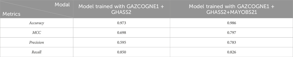
Table 9. Performance metrics of a YOLOv5 model (based on basic training set, Experiment #1) adapted to the MAYOBS23 data. Two models were used with different dataset combinations (Experiment #7). MCC stands for Matthews Correlation Coefficient.

The addition of MAYOBS21 data to the training set (i.e., EM122 Kongsberg WCIs not previously seen by the network) is not a pre-requirement for the network’s ability to detect fluids. However, the addition of MAYOBS21 significantly reduces the number of false positives. During the MAYOBS23 marine expedition, the GAZCOGNE1-GHASS2-MAYOBS21 model detected at least once 100% of the fluid emission sites that were independently identified by two operators. This number is higher than the recall (Table 9) due to the fact that each active site was surveyed at least twice. This test demonstrated that YOLOv5 performs effectively, consistently, and dependably in a monitoring mission when detecting all fluid-emission sites is crucial.

The MAYOBS23 marine expedition was an opportunity to deploy this model in near-real time acquisition. Onboard, access to raw data is possible once the acquisition file is closed. The first stage in MBES processing is the conversion from raw data to water column images (polar echograms) using Sonarscope software. This processing took approximately 1 min 28 s for a 42 Mo. all file on an 11th Gen Intel(R) Core (TM) i7-11850H processor. The second stage concerned the YOLOv5 processing whose speed was faster than the acquisition ping rate in the case of MAYOBS23. We approximated the acquisition rate by the delay between two pings of the sounder ∆T_ping by the equation (Equation 6) with c the speed of sound in water (1500 m·s^-1) and D_slant the maximum oblique distance between the MBES and seabed along extreme beams.

$∆Tping=\frac{2D_{slant}}{c}(6)$

The acquisition ping rate during MAYOBS23 given the water-depth range during MAYOBS23 and angular aperture (Table 1) ranges from 0.2 to 2.2 Image Per Second (IPS). The processing speed of YOLOv5 being faster (3.8 IPS in our case) than the maximum acquisition rate, YOLOv5 is suitable for online deployment. More details on the execution time of this method are given Supplementary Text S2.

4 Discussion

4.1 Major contributions of this new approach

The method developed in this study for fluid detection in multibeam-acquired images is based on the YOLOv5 model using enhanced training sets. This method overcomes some of the technological limitations encountered by previous methods. The method is scalable and reproducible on inference datasets, in contrast to single or multi-operator analysis, even if assisted by signal echo-integration (Dupré et al., 2014; Dupré et al., 2015) or 3D dB threshold filtering (Schneider von Deimling et al., 2015). Additionally, it enables detection under the Minimum Slant Range without relying on information from previous WCIs in the acquisition process (Urban et al., 2017; Weber, 2021). Finally, our method is adaptable to different seafloor morphologies (Table 1) and robust to non-stationary noise (and sidelobes) in comparison to Weber (2021). This method is also robust to other noise sources (e.g., dolphin echolocation, Supplementary Video S3).

Methodologically, the large databases, combined with the high variability and heterogeneity of water-column targets, acquisition parameters, MBES and environmental conditions, guarantee the robustness of results and provide a more comprehensive analysis of the method’s performance compared to previous studies performed by Zhao et al. (2020) and Mimura et al. (2023).

YOLOv5’s fast execution speed allowed for quick inference and processing on board. With a commonly used aperture of 120°, real-time YOLOv5 processing at shallow (150 m) and deeper water depths (1,500 m) is possible if we achieve a 2.5 and 0.3 IPS processing rate, respectively. This is possible with both the Central Processing Unit and the Graphical Processing Unit (3.8 and 41.7 IPS in our case, respectively) (Supplementary Text S2).

4.2 Out-performance of YOLOv5 compared to Haar-LBP

Based on the tested datasets, YOLOv5 clearly outperforms Haar-LBP in terms of robustness and reliability. Haar-LBP generates a significant number of false positives and a small number of false negatives on the very noisy GAZCOGNE1 dataset. It is hypothesized that this method is not very robust to noise. On the other hand, it produced a large number of false negatives and a few false positives on the high-resolution MBES dataset GHASS2, which suggests that the Haar-LBP model may not be suitable for narrow fluid-related echoes in the WCIs.

The superior performance of YOLOv5 on the GHASS2 dataset in comparison to GAZCOGNE1 can be attributed to the differences between the five GAZCOGNE1 folds used for cross-validation, which may have varying biomass contents (as detailed in Supplementary Table S2).

The metrics presented in Zhao et al. (2020) are impressive, likely due to i) their less noisy data, ii) larger fluid echoes compared to those from the GHASS2 dataset and iii) their evaluation protocol (e.g., balance between WCIs with and without fluid).

All the arguments support the use of the deep-learning based method (YOLOv5) over the shallow learning Haar-LBP; YOLOv5 being able to extract more relevant features for fluid detection.

4.3 Efficiently reducing false positives

Performance is primarily enhanced by adding WCIs, that contain non-fluid-related echoes through hard negative mining. This consists of adding a second labeled class of acoustic and environmental artefacts to the training set. Acoustic artefacts related to the MBES and other acoustic systems, environmental and background echoes (e.g., in our case, dolphin-echolocation echoes) are thus efficiently learnt by the YOLOv5 model by significantly reducing the number of false detections. To ensure accurate learning, it is secondly important to add WCIs without fluid with a diversity representative of the environmental variations that could be seen in the test set. The downside of adding WCIs without fluid is the increase in undetected actual fluids but this is negligible when considering the small number of WCIs concerned.

Performance can be thirdly enhanced by adding WCIs, that contain fluid-related echoes through pseudo-labeling, to the training set. However, there is only an improvement in the overall performance for the complex WCI dataset where fluid-related echoes are close or overlaid by other echoes that may exhibit similar acoustic signature (amplitude, shape) such as those produced by fish shoals. Adding WCIs with fluid to the training set is unnecessary in the case where the initial configuration dataset already contains a diverse range of fluid emissions that are suitable for accurate learning and generalization.

4.4 Learning from multiple acquisition modes

Including all the acquisition modes from the MBES in the training may result in a loss of performance (increase of FPs) in the case of fluid emissions restricted to water depth ranges predominantly surveyed with a single mode (as demonstrated for the “shallow” mode for the EM302 Kongsberg echosounder). In our studied case, we only used a testing set comprising WCIs acquired in shallow mode due to the restricted number of WCIs with fluid from medium and deep modes, which corresponds to 6% and 0% of all WCIs with fluid, respectively. In this case, learning from all acoustic modes may not be mandatory. However, as the distribution of potential fluid emissions is unknown for some exploratory expeditions, incorporating all acquisition modes in the training set (WCIs with fluid and without fluid) could enhance generalization.

In their 2024 study, Perret et al. did not specifically address the Kongsberg mode influence. However, they did utilize a training set comprising WCIs from two Kongsberg MBESs. This training set was composed of the following proportions: 36% shallow (only WCIs with fluid), 3% medium (less than 1% WCIs with fluid), 3% deep (no WCIs with fluid) for Kongsberg EM302, and 0% shallow, 8% medium, 18% deep for Kongsberg EM122 (WCIs with no fluid). The model trained is then able to detect 97% of fluid-related echoes on the Kongsberg EM122 PAMELA-MOZ1 dataset, whereas the corresponding WCIs were mainly acquired (99%) in the medium mode. This further supports the previous hypothesis, as the addition of different acoustic configurations to the training set enables the model to generalize, i.e., detect fluids from WCIs acquired in modes not previously seen.

Further investigations need to be conducted on the Kongsberg dataset including medium and deep mode acquisitions (e.g., EM302, EM122) to test and confirm this generalization hypothesis.

4.5 A multi-MBES fluid detector

4.5.1 Learning from combined-MBES dataset

Deep learning models are prone to overfitting, affecting generalization and predictive accuracy. To address this, we evaluated used cross-validation, and ensured strict training-test dataset separation. However, if a neural network is trained exclusively on data from a single MBES, it may struggle to generalize to other MBES systems, as demonstrated in Experiment #6, which involved cross-validation between the GHASS2 and GAZCOGNE1 datasets. These performance results suggest the model’s generalization is limited when applied to datasets with novel or significantly different characteristics (e.g., new echosounders or survey areas). Thus, the combination of several training datasets (GAZCOGNE1, GHASS2, MAYOBS21) from different MBES (Kongsberg EM302, Reson Seabat 7150, Kongsberg EM122) may significantly improve YOLOv5’s generalization capacity. For the GAZCOGNE1 inference, it is hypothesized that adding GHASS2 WCIs to the GAZCOGNE1 training set provides additional information for extracting and exploiting fluid features independently of the environment and sounder characteristics, even if the WCIs from the EM302 (GAZCOGNE1) and Seabat 7150 (GHASS2) are physically very different. Regarding the MAYOBS23 inference, we demonstrated that an accurate three-MBES-data-based model (GAZCOGNE1, GHASS2, MAYOBS21) can be trained with only a small number of WCIs from the EM122 (1,176 and 208 with and without fluid, respectively), efficiently resulting in minimal false negatives. This is crucial during exploration as it guarantees that fluid emissions do not go undetected. It is important to highlight that training with MAYOBS21 data primarily and drastically reduced the number of false positives identified by the network, which was already capable of detecting fluids on the EM122. This implies that incorporating these images primarily enables the network to learn the acoustic characteristics associated with the sounder as suggested by Perret et al. (2024). This demonstrates YOLOv5’s strong ability to learn from different MBES WCIs and to accurately generalize, eliminating the need for a dedicated MBES model. On the contrary, combining different training datasets may produce a higher number of FPs induced by precision reduction. In such a case (e.g., GHASS2 inference), it is likely due to the added GAZCOGNE1 information such as biomass or transmission sectors in the dataset which do not contribute to the network’s ability to learn fluid features on GHASS2 WCIs.

4.5.2 Retrain a network to detect fluid on a MBES using fluid features from the same or another MBES

In the present study, we constrained our approach to train the network with WCIs containing fluids from various multibeam echosounders, and subsequently perform inference on data derived from a MBES system included in the training set.

To delve further into this topic, Perret et al. (2024) explored training a YOLOv5 model without requiring fluid-labeled data from the specific MBES used for inference. To achieve this, a two-phase inference process was implemented. Initially, a network was trained with WCIs containing fluid-related echoes from the GHASS2 and GAZCOGNE1 datasets. This network was then used for inference on WCIs acquired during the first day of the PAMELA-MOZ1 campaign, which did not contain fluid-related echoes. This sub dataset included challenging data due to water-column echoes produced during coring operations and un-synchronized acoustic system surveys (i.e., subbottom profiler). Secondly, the WCIs incorrectly identified as containing fluids by the network were then incorporated into the training set (hard negative mining) (similarly to Experiment #4 of the present study conducted on Reson 7150 acoustic artefacts), also with other WCIs without fluid from the EM122 (similarly to Experiment #3). The network, trained with this training set, demonstrated the capacity to successfully learn features of fluid-related echoes from one MBES to another (97% of actual fluid emissions were detected), while simultaneously minimizing false detections (less than 1% of the entire cruise), even on a complex dataset (namely, with lots of acoustic artefacts). This means that the network was able to learn the characteristics of fluid echoes without relying on the sounder. This two-step learning methodology therefore exemplifies significant versatility across a variety of multibeam echosounder systems. Future studies could quantify the minimum number of WCI required to effectively adapt the model to new artefact types, which could, for example, facilitate rapid retraining during campaigns by leveraging outbound transit data.

4.6 Limitations

While this study achieves promising results, three key limitations present opportunities for future improvements.

This study highlights the need to enrich WCI datasets with diverse fluid information, environmental noise, and acoustic artifacts for improved underwater fluid emission detection. However, this analysis can always be expanded across specific new scenarios. Varying sonar operating modes (e.g., the medium and deep modes for Kongsberg acquisition), studying different natures of fluids (e.g., hydrothermal vents), or very shallow water depth environments (<100 m water depth) represent important areas for future exploration. Such investigations could provide more critical insights into the model’s adaptability to a wider range of marine environments.

The second limitation pertains to using uncalibrated data due to the paucity of information of the MBESs employed. Addressing the challenge of ensuring that the neural network remains invariant to these variations while maintaining accurate seep detection, was a key focus in Experiments #6 and #7. This raises an important question: should calibrated or standardized data be used in such analyses? Investigating the impact of calibration and standardization on model performance represents a promising avenue for future research.

The third limitation pertains to the elements of our algorithm that seek to address the detection of fluid in ping after ping WCIs. Our study focused on detection versus non-detection, as pinpoint-only annotations prevent evaluating YOLOv5’s localization or bounding box linkage. Bottom currents can tilt fluid flows affecting their spatial characteristics. Transverse currents allow reliable detection while those aligned with the vessel’s trajectory may cause repeated detections of the same seep. This arises from the network’s independent processing of pings without spatial or temporal context. Future work could address the linking of detections across pings to improve seep localization and prevent models from confusing fluids with acoustical artefacts (e.g., ghost echoes due to beam pattern).

5 Conclusion

Based on our research findings, we propose several key recommendations to improve the acquisition and processing of WCI data, as well as to enhance the robustness of YOLOv5 training.

To conduct a water-column survey, it is crucial to ensure a sufficient ping rate to detect at least once fluids in overlaps of the main along-track beam at the depth where they are located (Urban et al., 2023). Our fluid detector must use the same format as the WCIs used to train the model, including whether to cut the WCI after seabed detection, using polar or Cartesian projection, and the same pre-processing steps. In our case, Sonarscope software was used to convert the WCIs before applying the neural network. According to the present study and Perret et al. (2024), an operational proposal would be to commence a survey campaign with labeled fluid datasets (previously acquired) from the same or another MBES. A second step would consist of including in the training newly-acquired acoustic data relative to the acoustic MBES configuration and representative of the acoustic landscape (related to biomass and external noise) as far as possible. This could correspond to 1 day of acquisition (e.g., the first day, Perret et al. (2024)) or a different duration depending on the variability of the acoustic context. Subsequently, a neural network would be trained on board using previously labeled fluid-data and a subdataset from the current MBES survey. This network would then be used and adapted to the acoustic context of the area, to attempt to robustly detect fluids present in the survey area of the mission.

The authors of YOLOv5 provide advice on GitHub for effective YOLOv5 training (Jocher, 2021). Regardless of the field of study, it is important to include varied images that accurately reflect the environment, including WCIs and acoustic settings. It is essential to label all classes of images to ensure successful training. The present study provides additional guidance to enhance the model’s performance. One of the best strategies used in this study is hard negative mining. Caution should be exercised however when adding a second “acoustic and environmental artefacts” class. If labels are not correctly assigned to their respective classes, such as fluids being placed in the “acoustic and environmental artefact” class, the training process will face significant challenges in converging. If the signals are sufficiently different and not mixed in the WCIs, using 50% of these images with the second class in the training set can significantly enhance network performance. In addition, it is recommended to include at least 5%–10% of WCIs without fluid-related echoes in the training set and at maximum 25%–30%, percentages for which the performance is maximized and plateauing. These images without fluid are usually abundant and easy to obtain, and their inclusion will significantly help the network to better understand the environmental information not related to fluids. These images without fluid can also be used to decrease the number of detections made by the network; the more images without fluid-related echoes, the fewer false or accurate detections. The selection of the percentage of images without fluid echoes should be considered in light of the user’s needs. For the number of fluid-related echoes to train the network, we recommend using (with expert labeling and pseudo-labeling done with YOLOv5) approximately 2,700 labels for each type of echosounder data as we did see a significant improvement with the addition of 500 WCIs with fluid for GAZCOGNE1 (to the training set with already 2,214 WCIs with fluid-related echoes). The requisite number of WCIs with fluid may be less than previously assumed, as evidenced by GHASS2, where the metrics exhibit a plateau after the initial configuration (2,352 WCIs with fluid). This training dataset already contains a diverse range of fluid emissions that are suitable for accurate learning and generalization. The authors of YOLOv5 suggest using at least 10,000 items per category, which is significantly more than what was used in our study. This discrepancy can be attributed to the restricted number of classes and the relative simplicity of the objects present in WCIs in comparison to optical images. If one needs to use a specific sounder and only has a few WCIs with fluid-related echoes, it may not be possible to train a network solely with this data. It is however feasible to incorporate WCIs from various multibeam echosounders into a training set. Therefore, it is possible to include WCIs with fluid-related echoes from another sounder in larger quantities and WCIs without fluid-related echoes from the sounder of interest (Perret et al., 2024). This will enable the network to identify more general features from the WCIs and to use fluid features from another MBES. This will result in a network that is not perfect, but can still help the user by significantly reducing the number of WCIs requiring human inspection.

The present study focused on the use and performance of a supervised deep learning algorithm that can automatically detect and locate fluid emissions in WCIs. To date, automatic detection of these fluid emissions was indeed not very robust, even with existing methods. We demonstrated that using a deep learning-based method such as YOLOv5 is a more reliable algorithm for fluid detection than a shallow learning method like Haar-LBP. The network’s performance is greatly enhanced by modifying the acoustic composition of the YOLOv5 training sets. Thus, prioritizing examples of echoes that should not be detected (acoustic and environmental artefacts; e.g., data loss, multiple seafloor echoes and sounder artefacts) by creating a distinct class and using hard negative mining contribute to significantly decrease the number of false positives. Adding WCIs without fluid-related echoes also reduces false positives during inference. The addition of only a relatively small amount of WCIs with fluid (e.g., 500) through pseudo-labeling may improve the model’s performance but no longer beyond a certain threshold, which varies depending on the complexity of the data.

The present study demonstrated the feasibility of obtaining an efficient multi-MBES fluid detector able to detect different targets, namely, gaseous methane and carbon dioxide liquid. This detector can be adapted to different contexts with minimal effort, ensuring reliability. This detector can be used either in near-real-time acquisition aboard vessels (at a higher speed than the acquisition rate) or in post-acquisition conditions. The model weights and accompanying code for inference on raw multibeam echosounder data are publicly available in the Perret et al. (2025a), Perret et al. (2025b) repositories, providing a resource for reproducibility and further research.

Data availability statement

The datasets presented in this study can be found in online repositories. The names of the repository/repositories and accession number(s) can be found below: https://campagnes.flotteoceanographique.fr/campagnes/18001358/, https://campagnes.flotteoceanographique.fr/campagnes/13020070/, https://campagnes.flotteoceanographique.fr/campagnes/18002494/, https://github.com/perrettymea/YOLO-WAL-fluid-detection-WCI-data https://www.seanoe.org/data/00923/103,478/.

Author contributions

TP: Conceptualization, Formal Analysis, Methodology, Validation, Writing–original draft. GL: Funding acquisition, Supervision, Writing–review and editing, Conceptualization. AG: Writing–review and editing. YL: Writing–review and editing. SD: Funding acquisition, Resources, Supervision, Validation, Writing–review and editing, Conceptualization.

Funding

The author(s) declare that financial support was received for the research, authorship, and/or publication of this article. The GAZCOGNE1 marine expedition was part of the PAMELA project and was co-funded by TotalEnergies and IFREMER for the exploration of continental margins. The GHASS2 marine expedition was co-funded by the Agence Nationale de la Recherche for the BLAck sea MEthane (BLAME) project and IFREMER. MAYOBS21 and 23 were conducted by several French research institutions and laboratories, namely IPGP, CNRS, BRGM, and IFREMER. The project was funded by the Mayotte volcanological and seismological monitoring network (REVOSIMA), a partnership between IPGP, BRGM, OVPF-IPGP, CNRS, and IFREMER. This study presents the findings of a PhD project that was funded by IFREMER and the Brittany region through an ARED grant.

Acknowledgments

We wish to express our gratitude to the officers and crews of the research vessels Le Suroît, Pourquoi pas ?, and Marion Dufresne, as well as the technical staff from Genavir and Ifremer. The authors express sincere gratitude to Alison Chalm for revising the English language.

Conflict of interest

Author YL was employed by company Kongsberg Discovery.

The remaining authors declare that the research was conducted in the absence of any commercial or financial relationships that could be construed as a potential conflict of interest.

Generative AI statement

The authors declare that no Generative AI was used in the creation of this manuscript.

Publisher’s note

All claims expressed in this article are solely those of the authors and do not necessarily represent those of their affiliated organizations, or those of the publisher, the editors and the reviewers. Any product that may be evaluated in this article, or claim that may be made by its manufacturer, is not guaranteed or endorsed by the publisher.

Supplementary material

The Supplementary Material for this article can be found online at: https://www.frontiersin.org/articles/10.3389/frsen.2025.1532714/full#supplementary-material

References

Augustin, J.-M. (2023). Sonarscope software. SEANOE. doi:10.17882/87777

CrossRef Full Text | Google Scholar

Bochkovskiy, A., Wang, C., and Liao, H. M. (2020). YOLOv4: optimal speed and accuracy of object detection. CoRR, 10934. abs/2004. doi:10.48550/arXiv.2004.10934

CrossRef Full Text | Google Scholar

Chicco, D., Warrens, M., and Jurman, G. (2021). The Matthews Correlation Coefficient (MCC) is more informative than Cohen’s Kappa and Brier score in binary classification assessment. IEEE Access 9, 78368–78381. doi:10.1109/ACCESS.2021.3084050

CrossRef Full Text | Google Scholar

Clay, C. S., Medwin, H., and Urick, R. J. (1978). Acoustical oceanography: principles and applications. Phys. Today 31 (5), 71–73. doi:10.1063/1.2995042

CrossRef Full Text | Google Scholar

Dupré, S., Berger, L., Bouffant, N. L., Scalabrin, C., and Bourillet, J.-F. (2014). Fluid emissions at the Aquitaine Shelf (Bay of Biscay, France): a biogenic origin or the expression of hydrocarbon leakage? Cont. Shelf Res. 88, 24–33. doi:10.1016/j.csr.2014.07.004

CrossRef Full Text | Google Scholar

Dupré, S., Loubrieu, B., Pierre, C., Scalabrin, C., Guérin, C., Ehrhold, A., et al. (2020). The Aquitaine shelf edge (Bay of Biscay): a primary outlet for microbial methane release. Geophys. Res. Lett. 47 (7). doi:10.1029/2019GL084561

CrossRef Full Text | Google Scholar

Dupré, S., Scalabrin, C., Grall, C., Augustin, J. M., Henry, P., Celal, Ş. A. M., et al. (2015). Tectonic and sedimentary controls on widespread gas emissions in the Sea of Marmara: results from systematic, shipborne multibeam echosounder water column imaging. J. Geophys. Res. Solid Earth 120 (5), 2891–2912. doi:10.1002/2014JB011617

CrossRef Full Text | Google Scholar

Feuillet, N., Jorry, S., Crawford, W. C., Deplus, C., Thinon, I., Jacques, E., et al. (2021). Birth of a large volcanic edifice offshore Mayotte via lithosphere-scale dyke intrusion. Nat. Geosci. 14, 787–795. doi:10.1038/s41561-021-00809-x

CrossRef Full Text | Google Scholar

Freund, Y., and Schapire, R. E. (1995). A decision-theoretic generalization of on-line learning and an application to boosting. J. Comput. Syst. Sci. 55 (1), 119–139. doi:10.1006/jcss.1997.1504

CrossRef Full Text | Google Scholar

Goodfellow, I., Bengio, Y., and Courville, A. (2016). Deep learning. MIT press.

Google Scholar

He, K., Gkioxari, G., Dollár, P., and Girshick, R. (2018). Mask R-CNN. ArXiv. doi:10.48550/arXiv.1703.06870

CrossRef Full Text | Google Scholar

ICES (2023). Working group for the Bay of Biscay and the iberian waters ecoregion (WGBIE). ICES Sci. Rep. doi:10.17895/ices.pub.23541168.v1

CrossRef Full Text | Google Scholar

Jocher, G. (2021). Ultralytics/YOLOv5: v6.0. doi:10.5281/zenodo.5563715

CrossRef Full Text | Google Scholar

Jorry, S., Paquet, F., and Lebas, E. (2022). MAYOBS23 cruise, marion Dufresne R/V. doi:10.17600/18002494

CrossRef Full Text | Google Scholar

Judd, A., and Hovland, M. (2007). Seabed fluid flow: the impact on geology, biology and the marine environment. Cambridge University Press. doi:10.1017/CBO9780511535918

CrossRef Full Text | Google Scholar

LeCun, Y., Bengio, Y., and Hinton, G. (2015). Deep learning. Nature 521 (7553), 436–444. doi:10.1038/nature14539

PubMed Abstract | CrossRef Full Text | Google Scholar

Lee, D.-H. (2013). Pseudo-label: the simple and efficient semi-supervised learning method for deep neural networks. ICML 2013 Workshop Challenges Represent. Learn. (WREPL).

Google Scholar

Leifer, I., Luyendyk, B. P., Boles, J., and Clark, J. F. (2006). Natural marine seepage blowout: contribution to atmospheric methane. Glob. Biogeochem. Cycles 20 (3). doi:10.1029/2005GB002668

CrossRef Full Text | Google Scholar

Lin, T., Maire, M., Belongie, S. J., Bourdev, L., Girshick, R., Hays, J., et al. (2014). Microsoft COCO: common objects in context. CoRR, 740–755. doi:10.1007/978-3-319-10602-1_48

CrossRef Full Text | Google Scholar

Liu, W., Anguelov, D., Erhan, D., Szegedy, C., Reed, S., Fu, C.-Y., et al. (2016). SSD: single shot MultiBox detector. Lecture Notes in Computer Science 9905, 21–37. doi:10.1007/978-3-319-46448-0_2

CrossRef Full Text | Google Scholar

Loubrieu, B. (2013). GAZCOGNE1 cruise, Le Suroît R/V. doi:10.17600/13020070

CrossRef Full Text | Google Scholar

Lurton, X., and Augustin, J.-M. (2010). A measurement quality factor for swath bathymetry sounders. IEEE J. Ocean. Eng. 35 (4), 852–862. doi:10.1109/JOE.2010.2064391

CrossRef Full Text | Google Scholar

Lurton, X., Lamarche, G., Brown, C., Lucieer, V., Rice, G., Schimel, A., et al. (2015). “Backscatter measurements by seafloor-mapping sonars,” in Guidelines and recommendations. Zenodo. doi:10.5281/zenodo.10089261

CrossRef Full Text | Google Scholar

Mayer, L., Li, Y., and Melvin, G. (2002). 3D visualization for pelagic fisheries research and assessment. ICES J. Mar. Sci. 59 (1), 216–225. doi:10.1006/jmsc.2001.1125

CrossRef Full Text | Google Scholar

McGinnis, D. F., Greinert, J., Artemov, Y., Beaubien, S. E., and Wüest, A. (2006). Fate of rising methane bubbles in stratified waters: how much methane reaches the atmosphere? J. Geophys. Res. Oceans 111 (C9). doi:10.1029/2005JC003183

CrossRef Full Text | Google Scholar

Mimura, K., Nakamura, K., Takao, K., Yasukawa, K., and Kato, Y. (2023). Automated detection of hydrothermal emission signatures from multi-beam echo sounder images using deep learning. IEEE J. Sel. Top. Appl. Earth Observations Remote Sens. 16, 2703–2710. doi:10.1109/JSTARS.2023.3247467

CrossRef Full Text | Google Scholar

Neubeck, A., and Van Gool, L. (2006). Efficient non-maximum suppression. 18th Int. Conf. Pattern Recognit. (ICPR’06) 3, 850–855. doi:10.1109/ICPR.2006.479

PubMed Abstract | CrossRef Full Text | Google Scholar

Pan, S. J., and Yang, Q. (2010). A survey on transfer learning. IEEE Trans. Knowl. Data Eng. 22 (10), 1345–1359. doi:10.1109/TKDE.2009.191

CrossRef Full Text | Google Scholar

Parkhi, O. M., Vedaldi, A., and Zisserman, A. (2015). “Deep face recognition,” in Procedings of the British machine vision conference 2015 (Swansea: British Machine Vision Association), 41.1–41.12. doi:10.5244/C.29.41

CrossRef Full Text | Google Scholar

Perret, T., Dupré, S., Gaillot, A., Ladroit, Y., and Le Chenadec, G. (2024). “Knowledge transfer for deep-learning gas-bubble detection in underwater acoustic data: exploring data in the Mozambique Channel,” in International conference on underwater acoustics (ICUA), 46. doi:10.25144/22271Pt1

CrossRef Full Text | Google Scholar

Perret, T., Le Chenadec, G., Gaillot, A., Ladroit, Y., and Dupré, S. (2025a). YOLO-WAL: fluid-emission detection by water-column acoustics and a deep learning-approach. SEANOE. doi:10.17882/103478

CrossRef Full Text | Google Scholar

Perret, T., Le Chenadec, G., Gaillot, A., Ladroit, Y., and Dupré, S. (2025b). YOLO-WAL: fluid-emission detection by water-column acoustics and a deep learning-approach (v1.0.2). Zenodo. doi:10.5281/zenodo.14712210

CrossRef Full Text | Google Scholar

Poncelet, C., Billant, G., Corre, M.-P., and Saunier, A. (2023). Globe (global oceanographic bathymetry explorer) software. SEANOE. doi:10.17882/70460

CrossRef Full Text | Google Scholar

Redmon, J., Divvala, S. K., Girshick, R. B., and Farhadi, A. (2015). You only look once: unified, real-time object detection. CoRR, 02640. doi:10.48550/arXiv.1506.02640

CrossRef Full Text | Google Scholar

Ren, S., He, K., Girshick, R. B., and Sun, J. (2015). Faster R-CNN: towards real-time object detection with region proposal networks. CoRR, 01497. doi:10.48550/arXiv.1506.01497

CrossRef Full Text | Google Scholar

Riboulot, V., Dupré, S., Ker, S., and Sultan, N. (2021). GHASS2 cruise, Pourquoi pas ? R/V. doi:10.17600/18001358

CrossRef Full Text | Google Scholar

Riboulot, V., Ker, S., Sultan, N., Thomas, Y., Marsset, B., Scalabrin, C., et al. (2018). Freshwater lake to salt-water sea causing widespread hydrate dissociation in the Black Sea. Nat. Commun. 9, 117. doi:10.1038/s41467-017-02271-z

PubMed Abstract | CrossRef Full Text | Google Scholar

Rinnert, E., Thinon, I., and Lebas, E. (2021). MAYOBS21 cruise, RV marion Dufresne, doi:10.17600/18001986

CrossRef Full Text | Google Scholar

Ruffine, L., Donval, J.-P., Croguennec, C., Bignon, L., Birot, D., Battani, A., et al. (2017). Gas seepage along the edge of the Aquitaine Shelf (France): origin and local fluxes. Geofluids 13, 1–13. doi:10.1155/2017/4240818

CrossRef Full Text | Google Scholar

Sahling, H., Römer, M., Pape, T., Bergès, B., Dos Santos Ferreira, C., Boelmann, J., et al. (2014). Gas emissions at the continental margin west off Svalbard during R/V Heinche cruise HE387. doi:10.1594/PANGAEA.834000

CrossRef Full Text | Google Scholar

Schneider von Deimling, J., Linke, P., Schmidt, M., and Rehder, G. (2015). Ongoing methane discharge at well site 22/4b (North Sea) and discovery of a spiral vortex bubble plume motion. Mar. Petroleum Geol. 68, 718–730. doi:10.1016/j.marpetgeo.2015.07.026

CrossRef Full Text | Google Scholar

Schroff, F., Kalenichenko, D., and Philbin, J. (2015). “FaceNet: a unified embedding for face recognition and clustering,” in 2015 IEEE conference on computer vision and pattern recognition (CVPR) (Boston, MA, USA: IEEE), 815–823. doi:10.1109/CVPR.2015.7298682

CrossRef Full Text | Google Scholar

Shrivastava, A., Gupta, A., and Girshick, R. (2016). Training region-based object detectors with online hard example mining. arXiv:1604.03540.

Google Scholar

Sih, I. (2017). “Système d’information halieutique,” in données de production et d’effort de pêche (SACROIS) - 2003-2017. doi:10.12770/3e177f76-96b0-42e2-8007-62210767dc07

CrossRef Full Text | Google Scholar

Stanchev, L., Egbert, H., and Ruttenberg, B. (2020). “Automating deep-sea Video annotation using machine learning,” in 2020 IEEE 14th international conference on semantic computing (ICSC) (San Diego, CA, USA: IEEE), 17–24. doi:10.1109/ICSC.2020.00010

CrossRef Full Text | Google Scholar

Talukder, A. R. (2012). Review of submarine cold seep plumbing systems: leakage to seepage and venting. Terra nova. 24 (4), 255–272. doi:10.1111/j.1365-3121.2012.01066.x

CrossRef Full Text | Google Scholar

Tonchia, H., and Parthiot, F. (1994). Wide swath bathymetry and imagery systems some users observations and thoughts. Proc. OCEANS’94 3, III/219–III/224. doi:10.1109/oceans.1994.364200

CrossRef Full Text | Google Scholar

Urban, P., Köser, K., and Greinert, J. (2017). Processing of multibeam water column image data for automated bubble/seep detection and repeated mapping: processing of multibeam water column image data. Limnol. Oceanogr. Methods 15 (1), 1–21. doi:10.1002/lom3.10138

CrossRef Full Text | Google Scholar

Urban, P., Veloso-Alarcón, M. E., and Greinert, J. (2023). Echo grid integration: a novel method for preprocessing multibeam water column data to quantify underwater gas bubble emissions. Limnol. Oceanogr. Methods 21 (7), 377–400. doi:10.1002/lom3.10552

CrossRef Full Text | Google Scholar

Veloso, M., Greinert, J., Mienert, J., and De Batist, M. (2015). A new methodology for quantifying bubble flow rates in deep water using splitbeam echosounders: examples from the Arctic offshore NW-Svalbard. Limnol. Oceanogr. Methods 13, 267–287. doi:10.1002/lom3.10024

CrossRef Full Text | Google Scholar

Weber, T. C. (2021). A CFAR detection approach for identifying gas bubble seeps with multibeam echo sounders. IEEE J. Ocean. Eng. 46 (4), 1346–1355. doi:10.1109/JOE.2021.3056910

CrossRef Full Text | Google Scholar

Weber, T. C., Mayer, L., Jerram, K., Beaudoin, J., Rzhanov, Y., and Lovalvo, D. (2014). Acoustic estimates of methane gas flux from the seabed in a 6000 km2 region in the Northern Gulf of Mexico. Geochem. Geophys. Geosystems 15 (5), 1911–1925. doi:10.1002/2014GC005271

CrossRef Full Text | Google Scholar

Wu, H., and Prasad, S. (2017). Convolutional recurrent neural networks for hyperspectral data classification. Remote Sens. 9 (3), 298. doi:10.3390/rs9030298

CrossRef Full Text | Google Scholar

Yagis, E., Atnafu, S. W., García Seco de Herrera, A., Marzi, C., Scheda, R., Giannelli, M., et al. (2021). Effect of data leakage in brain MRI classification using 2D convolutional neural networks. Sci. Rep. 11 (1), 22544. doi:10.1038/s41598-021-01681-w

PubMed Abstract | CrossRef Full Text | Google Scholar

Zhao, J., Mai, D., Zhang, H., and Wang, S. (2020). Automatic detection and segmentation on gas plumes from multibeam water column images. Remote Sens. 12 (18), 3085. doi:10.3390/rs12183085

CrossRef Full Text | Google Scholar

Zou, Z., Chen, K., Shi, Z., Guo, Y., and Ye, J. (2023). Object detection in 20 years: a survey. Proc. IEEE 111 (3), 257–276. doi:10.1109/JPROC.2023.3238524

CrossRef Full Text | Google Scholar

Zurowietz, M., Langenkämper, D., Hosking, B., Ruhl, H. A., and Nattkemper, T. W. (2018). MAIA—a machine learning assisted image annotation method for environmental monitoring and exploration. PLOS ONE 13 (11), e0207498. doi:10.1371/journal.pone.0207498

PubMed Abstract | CrossRef Full Text | Google Scholar