
94% of researchers rate our articles as excellent or good
Learn more about the work of our research integrity team to safeguard the quality of each article we publish.
Find out more
ORIGINAL RESEARCH article
Front. Remote Sens. , 21 March 2025
Sec. Data Fusion and Assimilation
Volume 6 - 2025 | https://doi.org/10.3389/frsen.2025.1531097
 Andy Stock1,2*
Supervised learning allows broad-scale mapping of variables measured at discrete points in space and time, e.g., by combining satellite and in situ data. However, it can fail to make accurate predictions in new locations without training data. Training and testing data must be sufficiently separated to detect such failures and select models that make good predictions across the study region. Spatial block cross-validation, which splits the data into spatial blocks left out for testing one after the other, is a key tool for this purpose. However, it requires choices such as the size and shape of spatial blocks. Here, we ask, how do such choices affect estimates of prediction accuracy? We tested spatial cross-validation strategies differing in block size, shape, number of folds, and assignment of blocks to folds with 1,426 synthetic data sets mimicking a marine remote sensing application (satellite mapping of chlorophyll a in the Baltic Sea). With synthetic data, prediction errors were known across the study region, allowing comparisons of how well spatial cross-validation with different blocks estimated them. The most important methodological choice was the block size. The block shape, number of folds, and assignment to folds had minor effects on the estimated errors. Overall, the best blocking strategy was the one that best reflected the data and application: leaving out whole subbasins of the study region for testing. Correlograms of the predictors helped choose a good block size. While all approaches with sufficiently large blocks worked well, none gave unbiased error estimates in all tests, and large blocks sometimes led to an overestimation of errors. Furthermore, even the best choice of blocks reduced but did not eliminate a bias to select too complex models. These results 1) yield practical lessons for testing spatial predictive models in remote sensing and other applications, 2) highlight the limitations of model testing by splitting a single data set, even when following elaborate and theoretically sound splitting strategies; and 3) help explain contradictions between past studies evaluating cross-validation methods and model transferability in remote sensing and other spatial applications of supervised learning.
Supervised learning is a critical tool for mapping environmental variables like marine chlorophyll a, land cover types, and species distributions at broad spatial scales (Elith and Leathwick, 2009; Kerr and Ostrovsky, 2003; Tuia et al., 2022). In supervised learning, training a model involves extracting relationships between output (response) and input (predictor) variables from example data. In this way, supervised learning allows the continuous mapping of variables measured at discrete points in space and time. In marine satellite remote sensing, which serves as a case study here, common supervised learning approaches range from simple linear regression (e.g., Darecki et al., 2005; Kratzer et al., 2003; O'Reilly et al., 1998; O'Reilly and Werdell, 2019) to complicated machine learning methods (e.g., Kattenborn et al., 2021; Yuan et al., 2020; Zhang et al., 2023).
These models typically rely on in situ observations of the response variable for training and validation. A sound sampling design is critical when collecting in situ data for this purpose (Rocha et al., 2020). However, collecting data at sea over broad spatial scales and according to a sound sampling design would be extremely expensive. Therefore, to obtain sufficiently large in situ data sets, many broad-scale marine studies rely on databases that compile measurements from individual field campaigns with different objectives and without an overarching sampling strategy. Such data often have substantial spatial biases, i.e., some places are well-covered by data, whereas others have little or no data (Boakes et al., 2010; Bowler et al., 2022; Stock and Subramaniam, 2020). The spatial biases in such databases pose a critical statistical challenge in supervised-learning-based marine remote sensing (Stock, 2022).
A key question about models intended to generate broad-scale maps is how well they make predictions across the whole region of interest, including data-poor subregions (Peterson et al., 2007; Qiao et al., 2019; Stock and Subramaniam, 2020; Yates et al., 2018). Researchers traditionally evaluate and compare models by randomly splitting the available data into a training set for fitting the model and a test (or validation) set for estimating its prediction accuracy (sometimes, an additional development set is used for model selection and fine-tuning). This split can be done once or repeatedly in cross-validation. However, evaluating models based on random splits produces misleading results in many remote sensing and other environmental applications that involve spatial data (Fourcade et al., 2018; Ploton et al., 2020; Roberts et al., 2017). In particular, environmental variables are often spatially autocorrelated (Legendre, 1993), making nearby observations dependent. Dependence between training and testing data violates a core assumption of many statistical methods (Arlot and Celisse, 2010; Nikparvar and Thill, 2021), causes the selection of too complex models that do not generalize well (Gregr et al., 2019), and is a key driver of data leakage, a common cause of wrong results in scientific applications of supervised learning (Kapoor and Narayanan, 2023).
Two factors exacerbate these statistical problems as the popularity of machine learning as a scientific tool is rising, and machine learning is claimed to be superior to simpler statistical approaches (Pichler and Hartig, 2023). First, machine learning models can easily pick up location-specific relationships that fail to transfer to new locations (Beery et al., 2018), yet such failures are missed when training and testing data come from the same locations (Stock et al., 2023). Second, machine learning methods are rarely tailored to the limitations of typical environmental data, such as autocorrelated observations taken near each other. Ideally, models intended to make predictions for data-poor locations or to yield generalizable insights should be tested with independent, out-of-distribution data (Araújo et al., 2005; Geirhos et al., 2020; Gregr et al., 2019), yet such data are rarely available.
When only a single data set is available for model training and testing, cross-validation can mimic tests with independent data and extrapolation to data-poor regions by separating training and testing data spatially, temporally, or in predictor space (Roberts et al., 2017; Wenger and Olden, 2012). However, separating training and testing data does not guarantee sound error estimates for two reasons. First, if some subregions of the study area have no data, error estimates calculated for held-out subregions with data are not necessarily valid for subregions without data (for a method to estimate the area where a cross-validated error estimate applies, see Meyer and Pebesma, 2021). Second, the data being split might contain non-spatial biases and shortcuts. A sound data separation strategy is therefore necessary, but not sufficient, to avoid data leakage and obtain sound estimates of a spatial model’s prediction accuracy (Kapoor and Narayanan, 2023; Stock et al., 2023).
Two main approaches exist for separating training and testing data spatially. First, one can leave out one observation at a time for testing and withhold all data within a spatial buffer around the test observation from training (Le Rest et al., 2013; 2014; Pohjankukka et al., 2017). Second, one can split the data into blocks based geographical space (block cross-validation; Roberts et al., 2017; Sweet et al., 2023). Spatial cross-validation strategies yield better error estimates under spatial dependence and are hence a key tool in many environmental applications (Bald et al., 2023; Crego et al., 2022; El-Gabbas et al., 2021; Smith et al., 2021; Stock et al., 2018). An R package for spatial cross-validation is available (Valavi et al., 2019). However, spatial cross-validation remains underused in marine remote sensing and requires methodological choices such as the size and shape of spatial blocks.
Here, we explore how such choices affect error estimates with synthetic data that mimic a marine remote sensing application. With this example, we aim to inform the evaluation of predictive models in applications that 1) use supervised learning in satellite remote sensing or to create other broad-scale maps from point data, 2) must split a single data set for training and testing, and 3) rely on point data that were collected without an overarching sampling strategy, e.g., obtained from databases combining measurements from many individual field campaigns. Specifically, we ask: How do block size, shape, the number of cross-validation folds, and assignment of blocks to folds affect prediction error estimates and model selection? Which of these choices is most important? Might such choices explain contradictory results between prior studies comparing spatial cross-validation methods and testing the spatial transferability of models?
To answer our research questions, we exploit synthetic data that mimic a remote sensing application in marine biology (Stock, 2022). These data cover the Baltic Sea in northern Europe from 2003 to 2019. They consist of many individual data sets (henceforth, subsets) with geographic points (measurement locations and dates only) extracted from an oceanographic database. Each data point contains a response variable (synthetic chlorophyll a concentration) and satellite-based predictors (remote sensing reflectance in different wavelength bands) for these locations and dates where actual, in situ chlorophyll measurements existed. With each subset, three models of different complexity were trained and evaluated with various cross-validation strategies. Using a synthetic response variable that was generated with a model instead of values measured in situ allowed for calculating the models’ “true” prediction error across the study region and period, which were compared to cross-validated estimates limited to using the subsets, i.e., locations and dates where real in situ data existed (Figure 1). Importantly, “true” error here refers to a model’s prediction error in its intended task (generating daily maps of synthetic chlorophyll a for the whole Baltic Sea), not its skill predicting real-world, in situ chlorophyll a concentration.
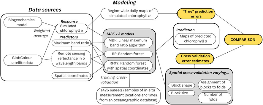
Figure 1. Overview of data sources and study design.
The synthetic data were developed in four steps outlined below to support the comparison of validation methods in a realistic use case of supervised learning. Additional details are provided in Stock (2022).
First, to create synthetic data with realistic distributions in space and time, we extracted locations and times of in situ chlorophyll a measurements from an oceanographic database (http://ocean.ices.dk/HydChem, accessed 31 August 2020). Such data are typically collected from ships during research cruises over many years. During cruises, researchers choose measurement locations based on the cruise’s scientific objectives instead of an overarching sampling strategy for the database. We excluded in situ measurement locations within 5 km from the coastline, made at depths >2 m, and with chlorophyll a concentrations >30 mg m−3.
Second, for predictors, each in situ observation was matched with satellite measurements of remote sensing reflectance in five wavelength bands (412 nm, 443 nm, 490 nm, 555 nm and 670 nm: http://globcolour.info, accessed 4 September 2020). The satellite data came from the GlobColour project, which combines data from several satellite-borne instruments to improve spatiotemporal coverage (Fanton d’Andon et al., 2009; Maritorena et al., 2010). The spatial resolution was 4km, and the temporal resolution was 1 day. Because clouds often obscure satellite views of the sea surface, many field observations had no matching satellite data. This reduces the number of usable observations and can introduce additional spatiotemporal biases due to uneven cloud cover (Stock et al., 2020). We matched the in situ and the satellite data with a same-calendar-day temporal window and bilinear interpolation from the four surrounding pixels, yielding 2,728 in situ observations with matching satellite data (henceforth, matchups: Figure 2A).
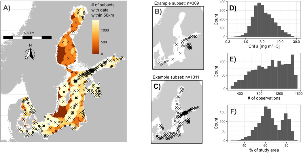
Figure 2. Map and selected statistics of the synthetic data used to evaluate cross-validation methods. (A) Locations of in situ observations of chlorophyll a with matching satellite data (which the subsets were sampled from) and the number of subsets that had observations within 50 km. (B, C) Two example subsets. (D) Histogram of synthetic chlorophyll a concentration used as response variable for the data from which the subsets were sampled. (E) Number of observations in the subsets. (F) Percent of the study area with at least one observation within 50 km across the generated subsets.
Third, to compare how well cross-validated error estimates approximated “true” prediction errors for the whole study region and period, the in situ chlorophyll a concentrations were replaced with synthetic values. These values were the weighted average of two sources with 4 km spatial and 1-day temporal resolution: 1) a biogeochemical simulation model of the Baltic Sea with 60% weight (Baltic Sea Biogeochemical Reanalysis, https://marine.copernicus.eu, accessed 31 August 2020), and 2) existing satellite-based maps of chlorophyll a, also from the GlobColour project, with 40% weight (these maps were previously generated with the same remote sensing reflectance data but another algorithm, and hence reflected some spatial patterns of the predictors). The averaging was necessary because simulated chlorophyll a was less correlated with remote sensing reflectance and with the original in situ measurements than in most real applications, whereas the satellite product could have been too easily reconstructed by flexible machine learning methods with remote sensing reflectance as predictors. The weights were chosen manually to correct for these unrealistically small correlations while keeping the biogeochemical simulation dominant (correlation of log10-transformed in situ chlorophyll with simulated values: Pearson correlation coefficient r = 0.16; with satellite chlorophyll from GlobColour: r = 0.49; with weighted average: r = 0.46). The Spearman rank correlation of the band ratio R (a common predictor of chlorophyll a, see section 2.3) with in situ chlorophyll a was ρ = 0.26, with simulated chlorophyll was ρ = 0.03, and with merged chlorophyll was ρ = 0.25. The moderate but significant (p < 0.001) correlations reflect high concentrations of other optical water constituents that make remote sensing of the Baltic Sea tricky (Darecki and Stramski, 2004; Siegel and Gerth, 2008; Stock, 2015). Furthermore, as is typical in real applications, the merged, synthetic chlorophyll a was roughly log-normally distributed (Figure 2D). Therefore, while chosen manually, the selected weights resulted in a synthetic response variable with statistical properties and relationships similar to the in situ measurements it replaced. Henceforth, “synthetic concentrations” refer to this weighted average.
Fourth, to create many synthetic yet realistic data sets with different sizes and spatial biases, 2000 random subsets were sampled from the 2,728 matchups (Figures 2B, C). To mimic oceanographic data collection, whole cruises were sampled (not individual observations). However, the automatic generation of spatial blocks with a common R package (Valavi et al., 2019) included in our test of cross-validation approaches failed for larger blocks in some small subsets (see Section 2.4). These subsets were excluded from the analyses to allow a comparison of all tested cross-validation methods. The remaining 1,426 subsets contained between 200 and 1,500 observations and exhibited different degrees of spatial bias (Figures 2E, F).
With each subset, we trained and tested three predictive models common in marine remote sensing. The response was always synthetic, log10-transformed chlorophyll a, but the models used different predictors and underlying mathematical structures.
The first model was a simple linear model:
Here, RRSxxx is the remote sensing reflectance in the respective wavelength band. Such models are called maximum band ratio algorithms and are among the longest-established statistical models for mapping chlorophyll a from satellites (O’Reilly et al., 1998).
The second model was a random forest (RF) using remote sensing reflectances in different wavelength bands and the band ratio R as predictors. Random forests are a basic machine-learning approach. They consist of many regression trees (here: 300) fitted to bootstrap samples of the training data while using only some predictors when fitting each tree (Breiman, 2001). Random forests work well for smaller data sets with correlated predictors and are a common choice in remote sensing applications (Belgiu and Drăgu, 2016).
The third model was a random forest with projected X and Y coordinates as additional predictors (RFXY). These spatial predictors allow the model to harness spatial structures in the data for predictions (Zhang et al., 2023). However, including them risks overfitting the model to these structures and limits its applicability when spatial structures change over time, e.g., because of climate change. Stock (2022) found that including spatial coordinates in a random forest caused large prediction errors that spatial, temporal, and environmental block cross-validation methods underestimated. Hence, the RFXY model is a “worst case” illustrating the limits of estimating prediction errors with spatial block cross-validation.
We tested two kinds of spatial blocks: (1) blocks and folds automatically generated with the R package blockCV (Figures 3A–F; Valavi et al., 2019), and (2) blocks manually created for the Baltic Sea (Figures 3G–I).
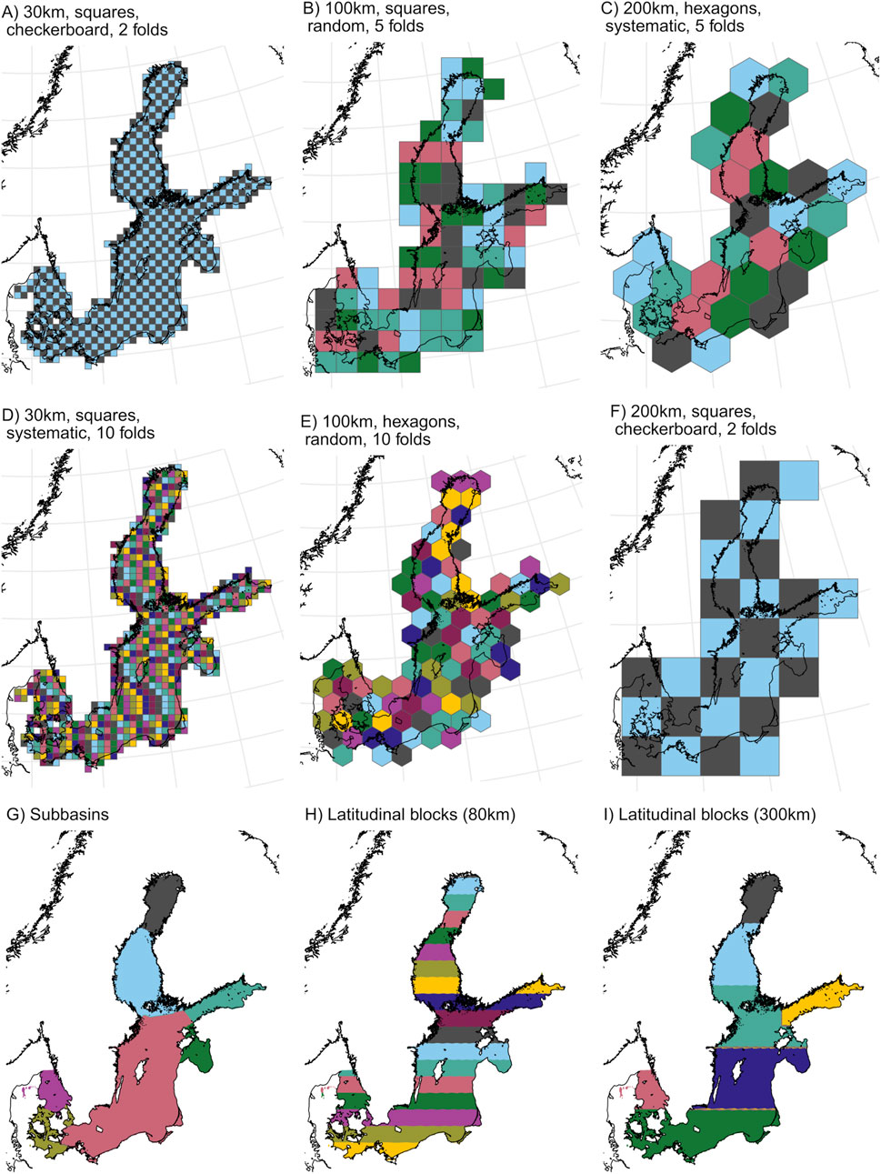
Figure 3. Examples of spatial blocks used for cross-validation. The blocks were either created automatically with the R package blockCV [examples in (A–F), with plot headings reflecting key parameters described in the text] or created manually for the Baltic Sea: subbasins (G) and latitudinal blocks reflecting environmental gradients in the study region (H, I).
The blockCV package allows the automatic generation of spatial blocks based on user-provided parameters. Here, we varied the following parameters: 1) block size (2 km–300 km); 2) block shape (squares or hexagons), 3) how blocks were assigned to folds (random, systematically, or in a checkerboard pattern), and 4) the number of folds (5 or 10 for random and systematic assignment, 2 for checkerboard assignment).
In addition, we manually created three sets of blocks. The first set was subbasins of the Baltic Sea, defined by HELCOM (the intergovernmental organization governing environmental issues in the Baltic Sea region). The second and third sets reflected the Baltic Sea’s environmental gradients from its connection with the Atlantic Ocean in the southwest to its northernmost bays, with north-south block sizes of 80 km and 200 km. In these manual designs, each block served as a fold. In each subset, folds with fewer than 20 observations were merged with the next-smallest fold until all blocks had at least 20 observations.
To be considered independent, training and testing data must be farther apart than the autocorrelation range (Trachsel and Telford, 2016). This range is thus critical information for spatial block cross-validation. It is traditionally estimated for residuals of the fitted model (Le Rest et al., 2014). However, fitting the model first precludes model selection, and residuals may be underestimated for flexible models overfitted to spatial structures (Roberts et al., 2017). Furthermore, with three models and 1,426 synthetic subsets, this study involved over 4,000 fitted models. Exploring residual autocorrelation for all was impractical. Consequently, we followed Valavi et al. (2019) and examined spatial autocorrelation of the predictors, assuming that they reflect the spatial structure of relevant environmental variables. Spatial autocorrelation can be examined, e.g., through variograms or correlograms, which provide similar information (Dormann et al., 2007). While variograms are a fundamental tool of geostatistics, correlograms are common in other fields like ecology and can be more robust when data are clustered (Wilde and Deutsch, 2006). Here, some clustering of available predictor data might have occurred because of differences in cloud cover across the study region. We hence calculated variograms as well as correlograms.
Spatiotemporal sample variograms were calculated for each predictor in two selected years (2005 and 2018) with the R package gstat (Gräler et al., 2016; Pebesma, 2012; Pebesma, 2004). For computational efficiency, each variogram calculation used a sample consisting of 5% pixels with data from the respective year. We calculated and averaged spatial correlograms with Moran’s I as a measure of spatial dependence for 100 randomly selected days during the study period with the R package ncf (Bjornstad, 2022).
Predictive models should be tested with data reflecting their target application (Kapoor and Narayanan, 2023). Because the target application was to create maps for the whole Baltic Sea, we compared cross-validated error estimates calculated with the spatial block options described in Section 2.4 and with standard 10-fold cross-validation to “true” prediction errors calculated for the whole study region and period. These “true” errors were calculated in three steps, as described below. Importantly, all prediction errors were calculated with the synthetic chlorophyll concentrations (which are known everywhere) as response variable. Hence, “true” refers to errors that are valid for the whole study region and period, not errors that reflect the real-world chlorophyll a concentration (which are only known where in situ data exist).
First, we trained each model (MBR, RF, RFXY) with each complete subset, i.e., without withholding any data from the subset (Kuhn and Johnson, 2013). Each subset contained synthetic chlorophyll a values as the response variable and the predictor variables as described in Section 2.2. This process yielded 4,278 trained models (three kinds of models trained on 1,426 subsets). Because the subsets were sampled from a database of field campaigns (see Section 2.2), training the models relied exclusively on locations and times where real in situ data existed.
Second, we created validation data covering the whole study region and period to calculate the “true” errors. Because making pixel-by-pixel predictions for 18 years of daily satellite data with over 4,000 models was computationally too expensive, we randomly sampled 1% of pixels in each daily satellite image. This sample comprised over 380,000 observations. Each observation contained a synthetic chlorophyll a value as response and predictor variables as described in Section 2.2. Hence, the data used to calculate “true” errors–in contrast to the test sets of the various cross-validation methods–contained observations from randomly sampled locations and times and covering the whole study region and period (as far as cloud cover allowed).
Third, with each of the 4,278 trained models, we made predictions for this test set covering the whole study region and period, yielding “true” error estimates in the sense that they reflected the purpose of broad-scale, satellite-based mapping precisely (making daily maps for the whole study region and period).
Finally, we applied the various cross-validation methods (Section 2.4) to each model and subset, resulting in 4,278 error estimates from each cross-validation method. Comparing these cross-validation estimates to the “true” errors revealed how well each method estimated the models’ prediction accuracy in the intended application.
As error measures, we used the root mean squared error (RMSE) and the absolute percentage difference (APD), calculated with the standard equations (like in Stock, 2022).
Synthetic chlorophyll a concentrations predicted with the MBR model had smaller “true” errors than those of the random forests (RF and RFXY) in 99% (RMSE) and 97% (APD) of subsets. Prediction errors were highest (1) in the Bothnian Bay, where the fewest training data were available (RMSE and APD) and (2) the eastern Gulf of Finland, the Gulf of Riga, and some smaller areas with very high synthetic chlorophyll a concentrations (RMSE only) (Figure 4). The APD’s comparatively small values in these high-chlorophyll areas might reflect this error measure’s low sensitivity to differences between larger numbers. Moderate “true” errors also occurred in large offshore areas where relatively low chlorophyll a concentrations and sparse data coverage coincided, like the Bothnian Sea (APD and RMSE).
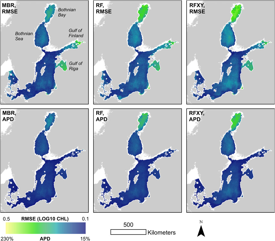
Figure 4. Spatial distribution of mean “true” errors (RMSE and APD of the three model types predicting synthetic chlorophyll a) averaged over 300 randomly sampled, partly cloud-free days across the whole study period. For each of the three model types, each subset yielded a different trained model, and prediction errors where averaged across subsets for this figure. “True” errors refers to errors when predicting synthetic chlorophyll a concentrations for the whole study region and period, not real-world concentrations.
The tested cross-validation methods often underestimated errors, especially for the RFXY model (Figure 5; Table 1). Overall, spatial block cross-validation yielded better error estimates than 10-fold cross-validation but sometimes overestimated errors. Error estimates from the blockCV package depended on the specific options, especially block size (see Section 3.2). They were larger than estimates from 10-fold cross-validation and smaller than estimates from large, manually created blocks (subbasins). Blocks generated with the blockCV package and good options led to a stronger underestimation than large manually created blocks in some cases but avoided an overestimation in others.
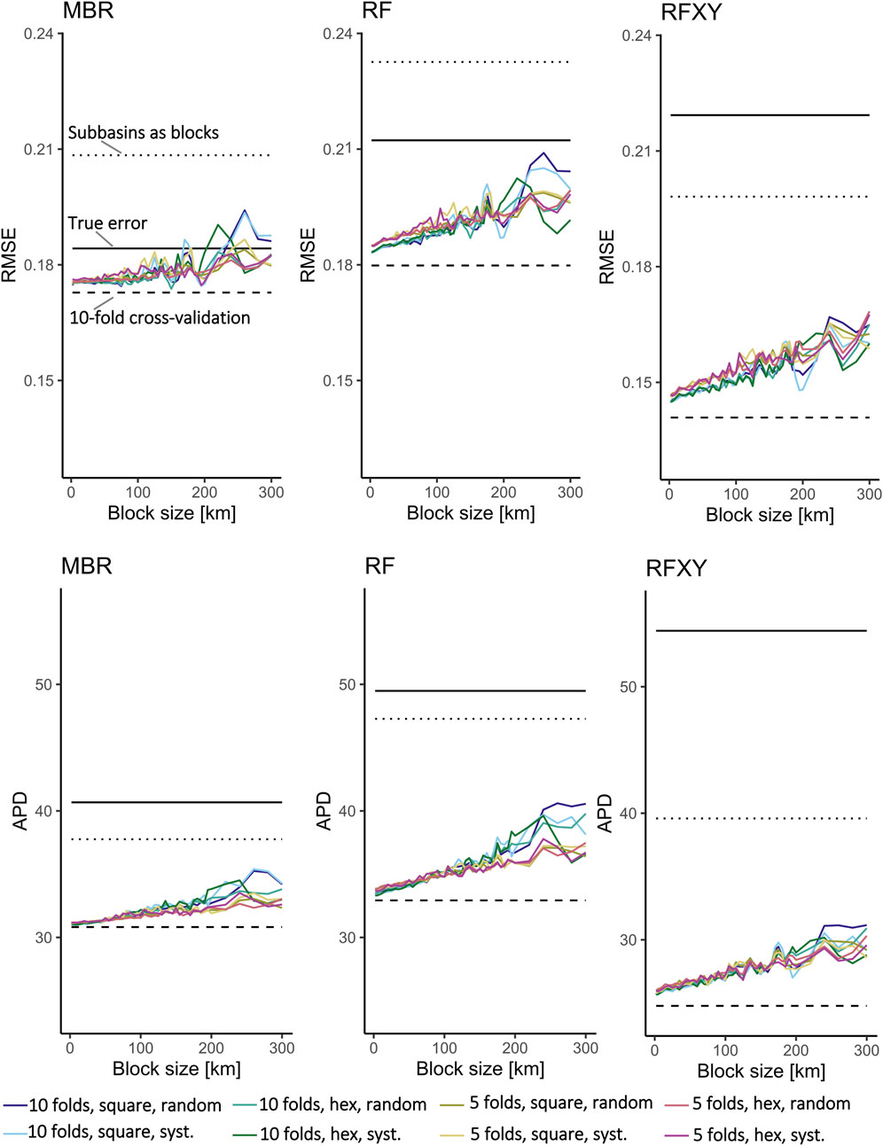
Figure 5. Estimated errors generated with different options in the blockCV R package as a function of block size. The solid black lines show the models’ “true” errors (mean error predicting synthetic Chl a concentration for the whole study region and period across all subsets). The dashed black line shows errors estimated with 10-fold cross-validation. The dotted line shows errors estimated using subbasins as spatial blocks.

Table 1. “True” errors and estimated errors with different cross-validation approaches. With the blockCV package’s various settings, there were too many combinations to show in the table. Instead, the table shows the best estimate obtained with the package (i.e., the one closest to the “true” error, representing an optimal choice of parameters) and the 25th percentile of absolute difference to the “true” error (P25, representing a good but not optimal choice of parameters). The estimates closest to the “true” errors are highlighted in bold font.
Depending on the model and error measure, 10-fold cross-validation underestimated prediction errors by 5% (RMSE of MBR) to 54% (APD of RFXY). The different block cross-validation methods yielded more accurate error estimates than 10-fold cross-validation, but the RMSE was sometimes overestimated. The best RMSE and APD estimates for RFXY were achieved with subbasins as blocks. The best APD estimates for MBR and RF were achieved by blocks generated with blockCV when optimal options were chosen; with solid but not optimal choice of options, the 80 km north-south blocks estimated the APD of these models best.
When choosing between the MBR and the RF models, all spatial cross-validation methods with large block sizes led to correct model selection for >98% of subsets. Ten-fold cross-validation selected the best model for fewer subsets (APD: 86%, RMSE: 93%). In contrast, model selection failed even with the best methods when choosing between all three models (MBR, RF, and RFXY). Ten-fold cross-validation incorrectly chose RFXY for over 99% of subsets. Spatial cross-validation with subbasins as blocks worked best, but RFXY was still incorrectly chosen in over 50% (APD) and 80% (RMSE) of subsets.
When creating square or hexagonal blocks automatically, choosing a large block size was the most important (Table 2). On average, cross-validation with ten folds yielded slightly better error estimates than five folds, square blocks yielded slightly better error estimates than hexagonal blocks, and systematic or checkerboard assignment of blocks to folds yielded slightly better error estimates than random assignment. However, except for the block size, the differences between the options were small. For example, averaged over all subsets and block sizes≥200 km, the random forest’s APD was underestimated by 25% with hexagonal blocks and 24% with square blocks. Nevertheless, large square blocks with systematic assignment to folds was always among the best choices, and often the best, across models and error measures (Figure 5).
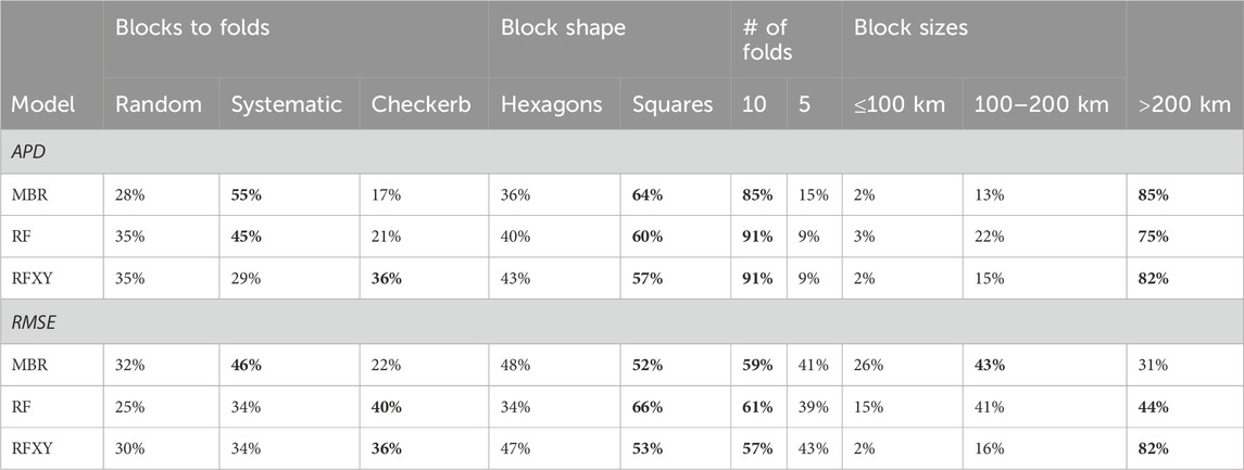
Table 2. Percentage of subsets for which different options were in the set of parameters yielding the most accurate blockCV-based error estimate. The highest percentages in each parameter group are shown in bold font.
Spatiotemporal variograms (Figure 6) showed that all predictors were spatially autocorrelated over several hundred kilometers, yet none of the variograms reached their sill within 500 km (already beyond a practical block size). Variograms calculated for 2005 (not shown) were similar to those for 2018. While correctly suggesting the need for large blocks to achieve independent training and testing data, the variograms did not suggest an optimal block size.
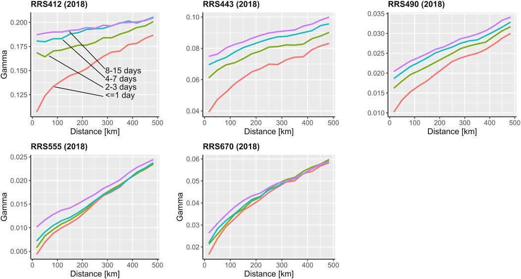
Figure 6. Empirical spatiotemporal variograms of the predictors for 2018.
Correlograms showed a more apparent autocorrelation range of the predictors (Figure 7). The spatial correlation dropped sharply within the first 100 km. It plateaued near 200 km for the 412 nm, 443 nm, and 490 nm wavelength bands and near 300 km for the 555 nm and 670 nm wavelength bands. Hence, the correlograms suggested a sound range for the block size in this application.
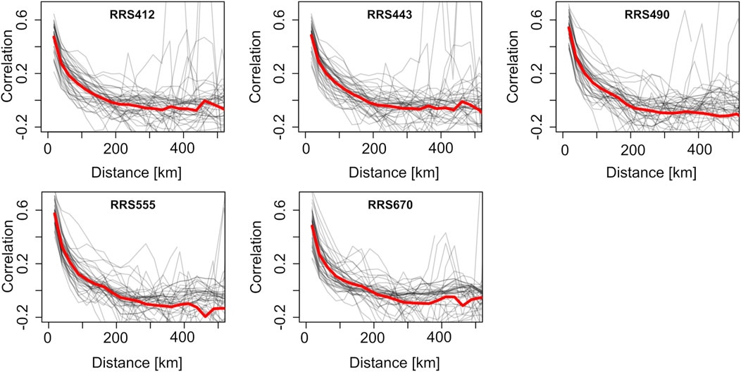
Figure 7. Correlograms for the predictors on 100 randomly sampled days (thin gray lines) and their average (thick black lines). On some days, there is no data for the largest distances shown due to cloud cover.
Several past studies have evaluated cross-validation methods with sometimes contradictory results.
On the one hand, several studies found that separating training and testing data spatially yields higher estimated errors than random data splits (Bahn and McGill, 2013; Karasiak et al., 2022; Meyer et al., 2018; 2019; Stock et al., 2018; Stock and Subramaniam, 2020). For example, Ploton et al. (2020) evaluated a random forest predicting above-ground forest biomass with random splits and two spatial cross-validation approaches. Random splits suggested good predictive skill, but spatial cross-validation suggested no predictive skill, reflecting the known effects of data leakage when training and testing data are insufficiently separated (Kapoor and Narayanan, 2023). Other tests with synthetic, autocorrelated data also show that error estimates from spatial block cross-validation are more accurate than random splits (Roberts et al., 2017; Stock, 2022). Furthermore, models selected with spatial block cross-validation can transfer better to new geographic locations (Tziachris et al., 2023). These prior results are consistent with this study.
On the other hand, several studies found that differences between spatial and random cross-validation were small and supported the same conclusions (Lyons et al., 2018; Valavi et al., 2023; Zhang et al., 2023). For example, Valavi et al. (2023) found that random and spatial block cross-validation yielded a similar ranking of models and that flexible models transferred well to new locations - contrary to, e.g., Gregr et al. (2019), where more flexible models failed when applied to independent data.
These prima facie contradictory results are explained by two aspects of the studies’ design. First, the studies used different block sizes–a critical choice according to our results. For example, Valavi et al. (2023) used a block size of 75 km to mimic extrapolation over comparatively short distances. As these authors correctly argue, results for extrapolation over larger distances might have been different. Second, spatial cross-validation is most important when data are unevenly distributed in space and time. For example, Lyons et al. (2018) compared cross-validation methods in a terrestrial vegetation mapping case study. They had a small study area (50 km2) and collected data specifically for their study with sound spatial sampling methods. Yet, with sound spatial sampling covering the whole study region, the biases of random cross-validation demonstrated in this and other studies become negligible, because randomly held-out test observations are not systematically farther from training observations than locations for which predictions are needed (Ramezan et al., 2019; Stock, 2022; Wadoux et al., 2021). In contrast, with data resembling the synthetic data here (i.e., databases that compile data from various sources without an overarching sampling strategy), cross-validation with random splits or too small blocks yields wrong error estimates.
Together, the importance of block size highlighted here and the spatiotemporal distribution of data adequately explain these contradictions in previously published research.
The most important parameter when automatically generating square or hexagonal blocks for spatial cross-validation was the block size. This choice is implicit but equally important when using existing regions as blocks (for example, when choosing between broad biogeographical regions or finer-scale subregions).
The first step in choosing a block size is analyzing spatial autocorrelation (Le Rest et al., 2014; Roberts et al., 2017). Here, correlograms showed autocorrelation ranges reflecting a suitable block size, whereas sample variograms showed that large blocks were needed but did not allow choosing a specific size. Hence, determining a good block size can require data exploration with several analytical tools. In addition, modelers must choose a cross-validation strategy that reflects the model’s intended application (Christin et al., 2020; Kapoor and Narayanan, 2023; Stock et al., 2023) – especially whether predictions beyond locations that are well-covered by data are needed.
Iterating over a plausible range of block sizes can yield additional insights, for example, exploring how error estimates change with increasing separation distance (Pohjankukka et al., 2017; Stock and Subramaniam, 2022). While a single set of manually crafted blocks is computationally more efficient and can reflect characteristics of the study region (such as biogeographical boundaries), an iterative approach avoids the need to select a block size a priori. Thus, it helps resolve situations where geostatistical analyses and domain knowledge do not clearly suggest which block size to use.
The block shape, the number of folds, and the assignment of blocks to folds were less important here, likely because they did not directly influence how the model testing reflected the target application. For example, while the spatial boundaries of statistical analysis units can affect results (the modifiable areal unit problem; Openshaw and Taylor, 1979), the shape of the blocks had minor effects on whether model testing reflected extrapolation to subregions without data. As another example, the number of folds influences the size of the training sets and, thus, the estimated prediction errors. The smallest data sets in this study had 200 observations. With 10 folds, each training set had 180 observations, and with 5 folds, 160 observations, with minor effects on the error estimates. While these options were unimportant here, they can matter in other applications. For example, it can be best to keep the training set as large as possible for very small data sets by using many folds or spatial buffers around single, held-out observations. Without such special considerations, when using a blocking strategy like those in the blockCV R package, square blocks, 10 folds, and systematic assignment of blocks to folds were good default choices.
This study’s main limitation is that it presents a single supervised learning application in one study region. Nevertheless, it can inform other applications because the results are theoretically plausible and sufficiently broad to explain apparent contradictions between prior studies (see Section 4.1). This study’s marine remote sensing example can, therefore, inform other supervised learning applications with spatially biased point data. However, like the conflicting past results discussed above, our recommendations’ relevance must be carefully judged in other applications and data contexts.
Environmental data might be autocorrelated in space and time, but this study tested only spatial blocks. Sweet et al. (2023) found that using clusters in predictor space as blocks worked best in a crop modeling example with spatiotemporal autocorrelation. In contrast, for synthetic chlorophyll a data like those used here, spatial blocks produced better error estimates than blocks in time or predictor space (Stock, 2022). Exploring the nuances of choosing spatial blocks was thus most critical for this study’s example application.
Basing the study on synthetic data allowed the evaluation of error estimates across the whole study region (not only locations where in situ data existed); such “simulation experiments” are a common tool to evaluate statistical methods (e.g., Dormann et al., 2012; Strobl et al., 2007; Roberts et al., 2017). However, simulated data from the biogeochemical model used to build the synthetic data was only weakly correlated with chlorophyll-a and a maximum band ratio, a key predictor in many chlorophyll remote sensing algorithms. This was alleviated by using a weighted average with an independent satellite data product, as opposed to the biogeochemical simulation results alone, as synthetic response variable. The synthetic data represented “real” marine remote sensing applications realistically for three reasons, hence allowing relevant insights into the performance of cross-validation methods. First, remote sensing reflectances and the band ratio serving as predictors were the same data used in many ocean color remote sensing studies. Second, the locations and dates of observations for model training and testing came from actual field campaigns, resampled to reflect the campaign-by-campaign growth of oceanographic databases. Third, the synthetic chlorophyll concentrations (averaged from biogeochemical simulations and a different satellite data product) had statistical properties similar to in situ chlorophyll concentrations. Therefore, the synthetic data were realistic regarding the predictors and the spatial and temporal distribution of data.
While focusing on a single study region, the Baltic Sea is typical for Case 2 waters, where remote sensing often relies on supervised learning with local to regional-scale data (Hafeez et al., 2019). Remote sensing reflectance is the foundation of many satellite algorithms besides mapping chlorophyll a. Therefore, the results are most relevant for other marine remote sensing applications in Case 2 waters.
The datasets presented in this study can be found in online repositories. The names of the repository/repositories and accession number(s) can be found below: https://figshare.com/s/132c0a410cc2800ca68f.
AS: Conceptualization, Data curation, Formal Analysis, Investigation, Methodology, Project administration, Resources, Software, Validation, Visualization, Writing–original draft, Writing–review and editing.
The author(s) declare that no financial support was received for the research and/or publication of this article.
The author declares that the research was conducted in the absence of any commercial or financial relationships that could be construed as a potential conflict of interest.
The author(s) declare that no Generative AI was used in the creation of this manuscript.
All claims expressed in this article are solely those of the authors and do not necessarily represent those of their affiliated organizations, or those of the publisher, the editors and the reviewers. Any product that may be evaluated in this article, or claim that may be made by its manufacturer, is not guaranteed or endorsed by the publisher.
Araújo, M. B., Pearson, R. G., Thuiller, W., and Erhard, M. (2005). Validation of species–climate impact models under climate change. Glob. Change Biol. 11 (9), 1504–1513. doi:10.1111/j.1365-2486.2005.01000.x
Arlot, S., and Celisse, A. (2010). A survey of cross-validation procedures for model selection. Stat. Surv. 4, 40–79. doi:10.1214/09-SS054A
Bahn, V., and McGill, B. J. (2013). Testing the predictive performance of distribution models. Oikos 122 (3), 321–331. doi:10.1111/j.1600-0706.2012.00299.x
Bald, L., Gottwald, J., and Zeuss, D. (2023). spatialMaxent: adapting species distribution modeling to spatial data. Ecol. Evol. 13 (10), e10635. doi:10.1002/ece3.10635
Beery, S., Van Horn, G., and Perona, P. (2018). “Recognition in terra incognita,” in Computer vision – eccv 2018. Editors V. Ferrari, M. Hebert, C. Sminchisescu, and Y. Weiss (Springer International Publishing), 472–489. doi:10.1007/978-3-030-01270-0_28
Belgiu, M., and Drăgu, L. (2016). Random forest in remote sensing: a review of applications and future directions. ISPRS J. Photogrammetry Remote Sens. 114, 24–31. doi:10.1016/j.isprsjprs.2016.01.011
Bjornstad, O. N. (2022). Ncf: spatial covariance functions. Available online at: https://CRAN.R-project.org/package=ncf.
Boakes, E. H., McGowan, P. J. K., Fuller, R. A., Chang-qing, D., Clark, N. E., O’Connor, K., et al. (2010). Distorted views of biodiversity: spatial and temporal bias in species occurrence data. PLOS Biol. 8 (6), e1000385. doi:10.1371/journal.pbio.1000385
Bowler, D. E., Callaghan, C. T., Bhandari, N., Henle, K., Benjamin Barth, M., Koppitz, C., et al. (2022). Temporal trends in the spatial bias of species occurrence records. Ecography 2022 (8), e06219. doi:10.1111/ecog.06219
Breiman, L. (2001). Random forests. Mach. Learn. 45 (1), 5–32. Article 1. doi:10.1023/a:1010933404324
Christin, S., Hervet, É., and Lecomte, N. (2020). Going further with model verification and deep learning. Methods Ecol. Evol. 12 (1), 130–134. doi:10.1111/2041-210X.13494
Crego, R. D., Stabach, J. A., and Connette, G. (2022). Implementation of species distribution models in google earth engine. Divers. Distributions 28 (5), 904–916. doi:10.1111/ddi.13491
Darecki, M., Kaczmarek, S., and Olszewski, J. (2005). SeaWiFS ocean colour chlorophyll algorithms for the southern Baltic Sea. Int. J. Remote Sens. 26 (2), 247–260. doi:10.1080/01431160410001720298
Darecki, M., and Stramski, D. (2004). An evaluation of MODIS and SeaWiFS bio-optical algorithms in the Baltic Sea. Remote Sens. Environ. 89 (3), 326–350. doi:10.1016/j.rse.2003.10.012
Dormann, C. F., Elith, J., Bacher, S., Buchmann, C., Carl, G., Carré, G., et al. (2012). Collinearity: a review of methods to deal with it and a simulation study evaluating their performance. Ecography 36 (1), 27–46. doi:10.1111/j.1600-0587.2012.07348.x
Dormann, C. F., Mcpherson, J. M., Arau, M. B., Bivand, R., Bolliger, J., Carl, G., et al. (2007). Methods Acc. spatial autocorrelation analysis species distributional data A Rev. doi:10.1111/j.2007.0906-7590.05171.x
El-Gabbas, A., Van Opzeeland, I., Burkhardt, E., and Boebel, O. (2021). Static species distribution models in the marine realm: the case of baleen whales in the Southern Ocean. Divers. Distributions 27 (8), 1536–1552. doi:10.1111/ddi.13300
Elith, J., and Leathwick, J. R. (2009). Species distribution models: ecological explanation and prediction across space and time. Annu. Rev. Ecol. Evol. Syst. 40 (1), 677–697. doi:10.1146/annurev.ecolsys.110308.120159
Fanton d’Andon, O., Mangin, A., Lavender, S., Antoine, D., Maritorena, S., Morel, A., et al. (2009). GlobColour—the European service for ocean colour. Proc. 2009 IEEE Int. Geoscience and Remote Sens. Symposium. doi:10.1029/2006JC004007
Fourcade, Y., Besnard, A. G., and Secondi, J. (2018). Paintings predict the distribution of species, or the challenge of selecting environmental predictors and evaluation statistics. Glob. Ecol. Biogeogr. 27 (2), 245–256. doi:10.1111/geb.12684
Geirhos, R., Jacobsen, J.-H., Michaelis, C., Zemel, R., Brendel, W., Bethge, M., et al. (2020). Shortcut learning in deep neural networks. Nat. Mach. Learn. 2, 665–673. doi:10.1038/s42256-020-00257-z
Gräler, B., Pebesma, E., and Heuvelink, G. (2016). Spatio-temporal geostatistics using gstat. R J. 8 (1), 204–218. doi:10.1007/978-3-319-17885-1
Gregr, E. J., Palacios, D. M., Thompson, A., and Chan, K. M. A. (2019). Why less complexity produces better forecasts: an independent data evaluation of kelp habitat models. Ecography 42, 428–443. doi:10.1111/ecog.03470
Hafeez, S., Wong, M., Ho, H., Nazeer, M., Nichol, J., Abbas, S., et al. (2019). Comparison of machine learning algorithms for retrieval of water quality indicators in case-II waters: a case study of Hong Kong. Remote Sens. 11 (6), 617. Article 6. doi:10.3390/rs11060617
Kapoor, S., and Narayanan, A. (2023). Leakage and the reproducibility crisis in machine-learning-based science. Patterns 4 (9), 100804. doi:10.1016/j.patter.2023.100804
Karasiak, N., Dejoux, J.-F., Monteil, C., and Sheeren, D. (2022). Spatial dependence between training and test sets: another pitfall of classification accuracy assessment in remote sensing. Mach. Learn. 111 (7), 2715–2740. doi:10.1007/s10994-021-05972-1
Kattenborn, T., Leitloff, J., Schiefer, F., and Hinz, S. (2021). Review on convolutional neural networks (CNN) in vegetation remote sensing. ISPRS J. Photogrammetry Remote Sens. 173 (July 2020), 24–49. doi:10.1016/j.isprsjprs.2020.12.010
Kerr, J. T., and Ostrovsky, M. (2003). From space to species: ecological applications for remote sensing. Trends Ecol. Evol. 18 (6), 299–305. doi:10.1016/S0169-5347(03)00071-5
Kratzer, S., Håkansson, B., and Sahlin, C. (2003). Assessing secchi and photic zone depth in the Baltic Sea from satellite data. Ambio 32 (8), 577–585. doi:10.1579/0044-7447-32.8.577
Legendre, P. (1993). Spatial autocorrelation: trouble or new paradigm? Ecology 74 (6), 1659–1673. doi:10.2307/1939924
Le Rest, K., Pinaud, D., and Bretagnolle, V. (2013). Accounting for spatial autocorrelation from model selection to statistical inference: application to a national survey of a diurnal raptor. Ecol. Inf. 14, 17–24. doi:10.1016/j.ecoinf.2012.11.008
Le Rest, K., Pinaud, D., Monestiez, P., Chadoeuf, J., and Bretagnolle, V. (2014). Spatial leave-one-out cross-validation for variable selection in the presence of spatial autocorrelation. Glob. Ecol. Biogeogr. 23 (7), 811–820. doi:10.1111/geb.12161
Lyons, M. B., Keith, D. A., Phinn, S. R., Mason, T. J., and Elith, J. (2018). A comparison of resampling methods for remote sensing classification and accuracy assessment. Remote Sens. Environ. 208 (February), 145–153. doi:10.1016/j.rse.2018.02.026
Maritorena, S., d’Andon, O. H. F., Mangin, A., and Siegel, D. A. (2010). Merged satellite ocean color data products using a bio-optical model: characteristics, benefits and issues. Remote Sens. Environ. 114 (8), 1791–1804. doi:10.1016/J.RSE.2010.04.002
Meyer, H., and Pebesma, E. (2021). Predicting into unknown space? Estimating the area of applicability of spatial prediction models. Methods Ecol. Evol. 12 (9), 1620–1633. doi:10.1111/2041-210x.13650
Meyer, H., Reudenbach, C., Hengl, T., Katurji, M., and Nauss, T. (2018). Improving performance of spatio-temporal machine learning models using forward feature selection and target-oriented validation. Environ. Model. and Softw. 101, 1–9. doi:10.1016/j.envsoft.2017.12.001
Meyer, H., Reudenbach, C., Wöllauer, S., and Nauss, T. (2019). Importance of spatial predictor variable selection in machine learning applications – moving from data reproduction to spatial prediction. Ecol. Model. 411, 108815. doi:10.1016/j.ecolmodel.2019.108815
Nikparvar, B., and Thill, J.-C. (2021). Machine learning of spatial data. ISPRS Int. J. Geo-Information 10 (9), 600. Article 9. doi:10.3390/ijgi10090600
Openshaw, S., and Taylor, P. (1979). “A million or so correlation coefficients: three experiments on the modifiable areal unit problem,” in Statistical applications in spatial sciences. London: Editor N. Wrigley (Pion), 127–144.
O’Reilly, J. E., Maritorena, S., Mitchell, B. G., Siegel, D. A., Carder, K. L., Garver, S. A., et al. (1998). Ocean color chlorophyll algorithms for SeaWiFS. J. Geophys. Res. Oceans 103 (C11), 24937–24953. doi:10.1029/98jc02160
O’Reilly, J. E., and Werdell, P. J. (2019). Chlorophyll algorithms for ocean color sensors—OC4, OC5 and OC6. Remote Sens. Environ. 229, 32–47. doi:10.1016/j.rse.2019.04.021
Pebesma, E. (2004). Multivariable geostatistics in S: the gstat package. Comput. Geosciences 30 (7), 683–691. doi:10.1016/j.cageo.2004.03.012
Pebesma, E. (2012). spacetime: spatio-temporal data in R. J. Stat. Softw. 51 (7), 1–30. doi:10.18637/jss.v051.i07
Peterson, A. T., Papeş, M., and Eaton, M. (2007). Transferability and model evaluation in ecological niche modeling: a comparison of GARP and Maxent. Ecography 30 (4), 550–560. doi:10.1111/j.0906-7590.2007.05102.x
Pichler, M., and Hartig, F. (2023). Machine learning and deep learning—a review for ecologists. Methods Ecol. Evol. 14 (4), 994–1016. doi:10.1111/2041-210X.14061
Ploton, P., Mortier, F., Réjou-Méchain, M., Barbier, N., Picard, N., Rossi, V., et al. (2020). Spatial validation reveals poor predictive performance of large-scale ecological mapping models. Nat. Commun. 11 (1), 4540. Article 1. doi:10.1038/s41467-020-18321-y
Pohjankukka, J., Pahikkala, T., Nevalainen, P., and Heikkonen, J. (2017). Estimating the prediction performance of spatial models via spatial k-fold cross validation. Int. J. Geogr. Inf. Sci. 31 (10), 2001–2019. doi:10.1080/13658816.2017.1346255
Qiao, H., Feng, X., Escobar, L. E., Peterson, A. T., Soberón, J., Zhu, G., et al. (2019). An evaluation of transferability of ecological niche models. Ecography 42 (3), 521–534. doi:10.1111/ecog.03986
Ramezan, C., Warner, A., and Maxwell, E. (2019). Evaluation of sampling and cross-validation tuning strategies for regional-scale machine learning classification. Remote Sens. 11 (2), 185. Article 2. doi:10.3390/rs11020185
Roberts, D. R., Bahn, V., Ciuti, S., Boyce, M. S., Elith, J., Guillera-Arroita, G., et al. (2017). Cross-validation strategies for data with temporal, spatial, hierarchical, or phylogenetic structure. Ecography 40 (8), 913–929. doi:10.1111/ecog.02881
Rocha, A. D., Groen, T. A., Skidmore, A. K., and Willemen, L. (2020). Role of sampling design when predicting spatially dependent ecological data with remote sensing. IEEE Trans. Geoscience Remote Sens. 59 (1), 663–674. doi:10.1109/tgrs.2020.2989216
Siegel, H., and Gerth, M. (2008). “Optical remote sensing applications in the Baltic Sea,” in Remote sensing of the European seas. Editors V. Barale,, and M. Gade (Springer), 91–102.
Smith, J. N., Kelly, N., and Renner, I. W. (2021). Validation of presence-only models for conservation planning and the application to whales in a multiple-use marine park. Ecol. Appl. 31 (1), e02214. doi:10.1002/eap.2214
Stock, A. (2015). Satellite mapping of Baltic Sea Secchi depth with multiple regression models. Int. J. Appl. Earth Observation Geoinformation 40, 55–64. doi:10.1016/j.jag.2015.04.002
Stock, A. (2022). Spatiotemporal distribution of labeled data can bias the validation and selection of supervised learning algorithms: a marine remote sensing example. ISPRS J. Photogrammetry Remote Sens. 187, 46–60. doi:10.1016/j.isprsjprs.2022.02.023
Stock, A., Gregr, E. J., and Chan, K. M. A. (2023). Data leakage jeopardizes ecological applications of machine learning. Nat. Ecol. and Evol. 7, 1743–1745. doi:10.1038/s41559-023-02162-1
Stock, A., Haupt, A. J., Mach, M. E., and Micheli, F. (2018). Mapping ecological indicators of human impact with statistical and machine learning methods: tests on the California coast. Ecol. Inf. 48, 37–47. doi:10.1016/j.ecoinf.2018.07.007
Stock, A., and Subramaniam, A. (2020). Accuracy of empirical satellite algorithms for mapping phytoplankton diagnostic pigments in the open ocean: a supervised learning perspective. Front. Mar. Sci. 7 (599). doi:10.3389/fmars.2020.00599
Stock, A., and Subramaniam, A. (2022). Iterative spatial leave-one-out cross-validation and gap-filling based data augmentation for supervised learning applications in marine remote sensing. GIScience and Remote Sens. 59 (1), 1281–1300. doi:10.1080/15481603.2022.2107113
Stock, A., Subramaniam, A., Van Dijken, G. L., Wedding, L. M., Arrigo, K. R., Mills, M. M., et al. (2020). Comparison of cloud-filling algorithms for marine satellite data. Remote Sens. 12 (20), 3313. doi:10.3390/rs12203313
Strobl, C., Boulesteix, A. L., Zeileis, A., and Hothorn, T. (2007). Bias in random forest variable importance measures: Illustrations, sources and a solution. BMC bioinformatics, 8, 1–21.
Sweet, L., Müller, C., Anand, M., and Zscheischler, J. (2023). Cross-validation strategy impacts the performance and interpretation of machine learning models. Artif. Intell. Earth Syst. 2 (4). doi:10.1175/AIES-D-23-0026.1
Trachsel, M., and Telford, R. J. (2016). Technical note: estimating unbiased transfer-function performances in spatially structured environments. Clim. Past 12, 1215–1223. doi:10.5194/cp-12-1215-2016
Tuia, D., Kellenberger, B., Beery, S., Costelloe, B. R., Zuffi, S., Risse, B., et al. (2022). Perspectives in machine learning for wildlife conservation. Nat. Commun. 13 (1), 792. Article 1. doi:10.1038/s41467-022-27980-y
Tziachris, P., Nikou, M., Aschonitis, V., Kallioras, A., Sachsamanoglou, K., Fidelibus, M. D., et al. (2023). Spatial or random cross-validation? The effect of resampling methods in predicting groundwater salinity with machine learning in mediterranean region. Water 15 (12), 2278. Article 12. doi:10.3390/w15122278
Valavi, R., Elith, J., Lahoz-Monfort, J. J., and Guillera-Arroita, G. (2019). blockCV: an r package for generating spatially or environmentally separated folds for k-fold cross-validation of species distribution models. Methods Ecol. Evol. 10 (2), 225–232. doi:10.1111/2041-210X.13107
Valavi, R., Elith, J., Lahoz-Monfort, J. J., and Guillera-Arroita, G. (2023). Flexible species distribution modelling methods perform well on spatially separated testing data. Glob. Ecol. Biogeogr. 32 (3), 369–383. doi:10.1111/geb.13639
Wadoux, A. M. J.-C., Heuvelink, G. B. M., de Bruin, S., and Brus, D. J. (2021). Spatial cross-validation is not the right way to evaluate map accuracy. Ecol. Model. 457, 109692. doi:10.1016/j.ecolmodel.2021.109692
Wenger, S. J., and Olden, J. D. (2012). Assessing transferability of ecological models: an underappreciated aspect of statistical validation. Methods Ecol. Evol. 3 (2), 260–267. doi:10.1111/j.2041-210X.2011.00170.x
Wilde, B., and Deutsch, C. V. (2006). Robust alternatives to the traditional variogram. CCG Annu. Rep. 116.
Yates, K. L., Bouchet, P. J., Caley, M. J., Mengersen, K., Randin, C. F., Parnell, S., et al. (2018). Outstanding challenges in the transferability of ecological models. Trends Ecol. and Evol. 33 (10), 790–802. doi:10.1016/j.tree.2018.08.001
Yuan, Q., Shen, H., Li, T., Li, Z., Li, S., Jiang, Y., et al. (2020). Deep learning in environmental remote sensing: achievements and challenges. Remote Sens. Environ. 241 (February), 111716. doi:10.1016/j.rse.2020.111716
Keywords: machine learning, satellite, ocean color, random forest, Baltic Sea, accuracy, autocorrelation, supervised learning
Citation: Stock A (2025) Choosing blocks for spatial cross-validation: lessons from a marine remote sensing case study. Front. Remote Sens. 6:1531097. doi: 10.3389/frsen.2025.1531097
Received: 19 November 2024; Accepted: 13 March 2025;
Published: 21 March 2025.
Edited by:
Tongwen Li, Sun Yat-sen University, ChinaCopyright © 2025 Stock. This is an open-access article distributed under the terms of the Creative Commons Attribution License (CC BY). The use, distribution or reproduction in other forums is permitted, provided the original author(s) and the copyright owner(s) are credited and that the original publication in this journal is cited, in accordance with accepted academic practice. No use, distribution or reproduction is permitted which does not comply with these terms.
*Correspondence: Andy Stock, YW5jQG5pdmEubm8=
Disclaimer: All claims expressed in this article are solely those of the authors and do not necessarily represent those of their affiliated organizations, or those of the publisher, the editors and the reviewers. Any product that may be evaluated in this article or claim that may be made by its manufacturer is not guaranteed or endorsed by the publisher.
Research integrity at Frontiers
Learn more about the work of our research integrity team to safeguard the quality of each article we publish.