Assessment of the application of each multibeam echosounder data product for monitoring of Laminaria digitata in the UK

Amid warming seas, high rates of pollution and declining fish stocks observed around the UK, the vital role of kelp as ecosystem mediators on our coastlines is increasingly significant; currently estimated at £500 billion. Extensive research on the rapid decline of kelp forests and its potential consequences has prompted the initiation of numerous conservation efforts. This research set out to determine the applicability and efficiency of a less invasive, remote sensing technique for monitoring kelp. A high resolution multibeam echosounder (MBES) survey was performed to acquire depths, backscatter and water column data in an area known to have kelp. An evaluation of different combinations of the MBES data products for kelp forest monitoring was carried out. An image-based processing methodology using a random forests algorithm was used to generate classification models, which were trained and tested using ground truth samples obtained through video imagery. This study reports climbing model accuracy scores from 62.2% (±11%, 1σ) to 90% (±10%, 1σ) on consecutive input of data products, indicating MBES as an effective tool with respect to other technologies. When considering practical difficulties associated with simultaneous record of all data products against their individual value, this study suggests that bathymetry and backscatter products deliver greatest value for distinction of small form kelp, while angular response analysis and water column data deliver lesser value but are required for optimised accuracy.

Introduction

The challenge to develop an effective and standardised approach to kelp forest monitoring is significant. In a period where global environmental health metrics are indicative of decline (Butchart et al., 2010), it is essential that strategies to monitor and support foundation species are prioritised. Unfortunately, society’s reduced exposure to marine ecosystems means that their value is generally overlooked (Townsend et al., 2018); few people realise the extent of the benefits reaped from our oceans. The lack of attention, compounded with the physical challenges associated with subsea monitoring, provides a clear motive for the development of an innovative solution.

It is estimated that kelp forests generate ∼$500 billion of natural capital value annually (Eger et al., 2023). This claim is substantiated by the environmental roles of kelp that include, but are not limited to, fixation of carbon to deep sea sinks (Wernberg et al., 2019; Filbee-Dexter et al., 2024), filtration and oxygenation of waters (Umanzor and Stephens, 2023), provision of habitats for aquatic life, and absorption of wave energy (Koehl, 1984; Morris et al., 2020). Global abundance of kelp is falling by ∼2% per annum (Wernberg et al., 2019), however some areas report losses of up to 90% in living memory (Eger et al., 2024). Decline is attributed to the increased ubiquity of the known stressors of kelp (Wear et al., 2023), which include overfishing, damaging fishing practices, warming seas, and polluted waters. Within the UK, conservation efforts such as the Sussex Kelp Recovery Project (SKRP) and the Great Yorkshire Kelp Recovery project have been launched within the worst affected areas where observational records indicate an almost complete loss of what were once thriving kelp populations – the reported success of these efforts depends partly on the effectiveness of the chosen monitoring approach.

Numerous remote sensing technologies have been explored for their applicability to kelp forest monitoring. Given the success of Satellite Imagery as a tool for leveraging photosynthesizers’ unique interactions with the visible spectrum to map terrestrial vegetation (Alam et al., 2020; Liu et al., 2019; Wulder et al., 2024), transferability to subsea photosynthesizers (including kelp) has been investigated. Reported accuracies of models for discrimination of expansive floating kelp forests derived from Satellite Imagery are in the range of 80%–90% (St-Pierre and Gagnon, 2020; Gendall et al., 2023). Low spatial and temporal resolution limit the applicability of this technology for monitoring of dynamic, small form and sparse kelp populations. Cameras deployed on divers or towed frames are common due to their affordability and ease of operation, however the poor coverage and qualitative nature of output data makes production of spatial distribution maps challenging. While automated image analysis of subsea imagery has proven effective in controlled environments (kelp farms) (Overrein et al., 2024), feature ambiguity in uncontrolled waters means the technology still requires human interpretation which is subjective in nature. Acoustic technologies benefit from the improved propagation of sound through water relative to light, and so constitute the bulk of the subsea surveyors’ toolbox.

This study explores the use of the multibeam echosounder as a tool for high resolution monitoring of kelp populations common to the UK’s coastline, with a focus on identifying the added value of each of the multibeam data products. Bathymetry, uncalibrated backscatter mosaics, angular response analysis (ARA), and water column (WC) data constitute the considered data products. While previous research indicates improvement of classification model performance on addition of each individual data product, variability of parameters across studies means the scale of improvements derived from each product cannot be compared. This research works to unify the assessment of all data products within a single study, enabling evaluation of their respective value.

MBES data was acquired in Lulworth Cove, situated on England’s south coast. 2D georeferenced grids were produced for each data product and used alongside ground truth data as input into a random forests (RF) algorithm. Generation, testing, and comparison of multiple models associated with different combinations of data product inputs with varying levels of smoothing provided an indication of the discriminatory power derived from each product. Through consideration of each product’s impact on model performance as well as the known challenges associated with their collection, this study aims to present pragmatic recommendations pertaining to design of an MBES survey for kelp monitoring applications in the UK. Additionally, this study aims to identify existing survey campaigns in the UK that could be leveraged, by virtue of their appropriate survey design (collection of the most valuable data products), to facilitate cost-effective provision of data for monitoring of kelp.

Methodology

Study site – Lulworth Cove

Lulworth Cove, situated on England’s south coast was selected as the study area for this research due to its sheltered nature, known presence of kelp, and good accessibility (Figure 1). Depths within the cove rarely exceed 5 m (below chart datum), with tides ranging between ∼0.4 m and ∼2 m during the week of data collection in June 2024. The cove is almost fully enclosed, with high cliffs providing good shelter from wind resulting in minimal swells which was ideal for data collection using a small USV. Through discussion with locals, a site visit, and evaluation of satellite imagery, it was evident that the site had a strong presence of kelp in the North West and South East of the cove, with areas of weed and sand distributed towards the centre. Reported kelp species include Laminaria digitata (Oarweed), Laminaria hyperborea (Forest Kelp), and Sacchoriza polyschides (Furbelows). Lulworth Cove is a tourist destination, with provision of easy access and amenities.

Figure 1

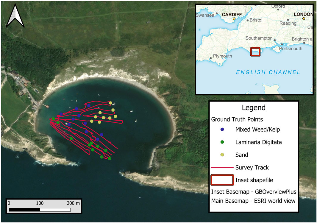
Figure 1. Map of the Survey site produced in QGIS using satellite imagery as well as Ordnance Survey’s GB overview product. Red lines show survey track, coloured points indicate the ground truth observations used.

Multibeam survey

Survey platform

The multibeam survey was conducted on the 26th of June 2024. The chosen survey vessel was the UCL Tamesis, a Maritime Robotics Otter USV, (Figure 2). The employment of the Tamesis was appropriate for the following reasons:

• Small draft of the Tamesis (∼15 cm) facilitates access to very shallow waters, improving survey coverage. For survey of sensitive environments, smaller craft could be considered less invasive. This is especially significant given kelp’s affinity to shoal rocks.

• Improved manoeuvrability. Small form relative to traditional craft allows access to confined spaces, again improving coverage

Figure 2

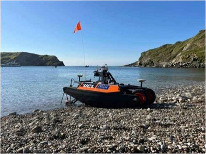
Figure 2. UCL Tamesis before launch from the beach at Lulworth Cove.

The Tamesis was equipped with a Norbit Winghead i80s multibeam sonar (which includes an integrated sound velocity probe and inertial measurement unit), a tightly coupled Applanix POS MV and a Valeport Swift sound velocity probe (lowered via winch). Maritime Robotics software was used for navigation, while data was collected in both BeamworX’s NavAQ software and Norbit’s proprietary user interface. Data was collected in two software packages given:

• Norbit’s s7k format is accepted by Espresso software (see data processing methodology)

• BeamworX’s NavAQ software provides numerous live data stream visualisations important for real time quality control

Survey design

Backscatter and water column data collection are optimised through slightly differing survey designs. An important consideration when recording all three data products simultaneously with a Norbit system is that water column is only collected for every 1 in 5 pings. In the interest of time, a single survey was performed, with the following configuration based on recommendations from equipment manuals and the literature (Norbit, 2024).

A larger swath overlap is especially advantageous for backscatter data collection, as it ensures that areas are ensonified by pings at various angles of incidence. This variability can then enhance the accuracy of ARA. This is also a fundamental method for ensuring data quality through cross validation of adjacent lines, as such 100% overlap was targeted. Additionally, sharp turns were avoided due to the associated loss of data at the outside extents of the swath.

Survey from multiple directions is common for a standard bathymetric survey to facilitate further cross validation, however, this approach results in ensonification from many different perspectives - this has been known to reduce coherence of backscatter data (Lamarche and Lurton, 2018; Lurton et al., 2018) (especially for areas of complex bathymetry such as Lulworth) as artefacts of inaccurate backscatter slope correction begin to accrue. In practice, the achievement of the above targets was variable largely due to challenges including obstacles such as boats, mooring lines and swimmers as well as the effect of tidal currents and swell on vessel navigation. Figure 1 shows the post processed vessel trajectory with the aim to visualise deviations from the survey plan.

Multibeam echosounder configuration

Through the Norbit user interface, key parameters were set as shown in Table 1.

Table 1

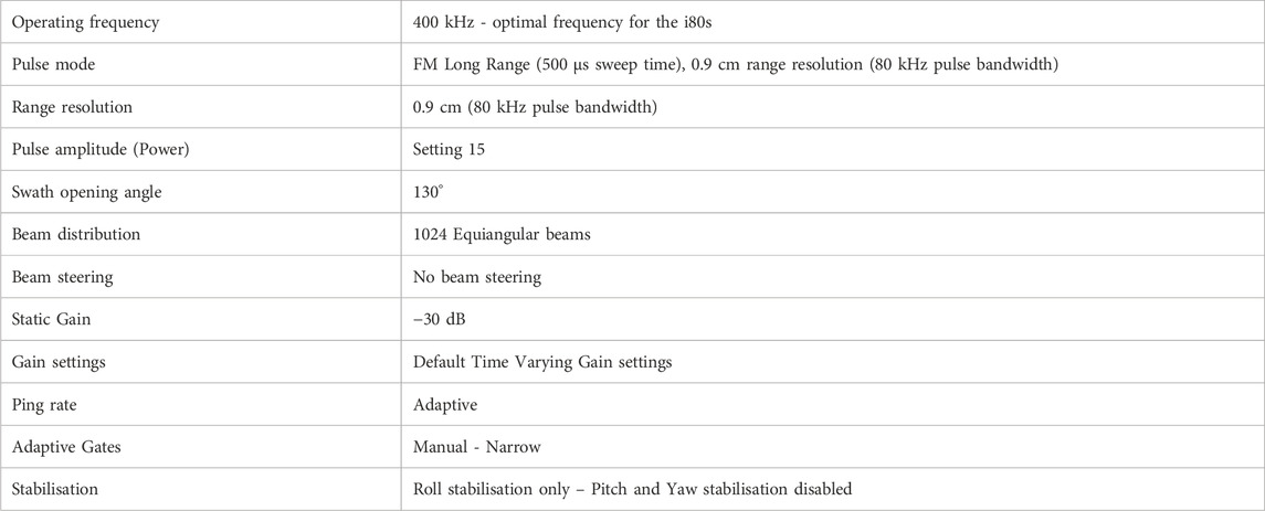
Table 1. Summary of key MBES configuration parameters.

Ensuring sweep time is constant through the survey is of particular importance for backscatter surveys. The default Auto mode will jump between sweep times, complicating data processing (Norbit, 2024).

GNSS sensors for absolute georeference

For absolute georeferencing of the Norbit system, and therefore the soundings, Applanix GNSS receivers were used alongside Norbit’s integrated IMU. Due to the steep cliffs surrounding the cove, no mobile data was available, resulting in a reliance on standard differential GNSS corrections (encoded within the satellite transmission signal). 3D position was initially referenced in WGS84 (ESPG: 4326) prior to transfomation to OSGB36 (ESPG: 27700) with Ordnance Datum Newlyn. OSTN15 and OSGM15 models were used to derive horizontal and vertical reference, respectively.

Sound velocity measurements

The cove receives inflow from a small freshwater stream to the North, introducing some level of freshwater/saltwater mixing. Given the contrasting properties of each water body and their impact on acoustic propagation, it is important that mixing is modelled to appropriately calculate the path and speed of the sound waves within the water column. It is especially important to measure frequent sound velocity (SV) profiles in this environment given the dynamic effect of the flooding and ebbing tide on freshwater mixing. The sound velocity probe was therefore deployed via the onboard winch every 30 minutes and the recorded profiles were imported into NavAQ for live corrections. Six dips were taken with minimal observed variation in SV.

Ground truth survey

The ground truth survey was performed on the 5th of July 2024. A remote sensing approach (video imagery) was taken for ground truthing (over traditional grab sampling approaches) to reduce impact on the environment and simplify both acquisition and processing. A small (∼2 m) inflatable vessel was used to navigate the site, while a weighted line was used to lower a GoPro Hero 5 Session to the seabed. Video was recorded to provide both the local bed type and contextual information (water column and surrounding area). To combat light attenuation, survey was performed near low tide to improve natural light, and an LED panel was appended to the camera line. Sample sites were selected at graduated distances along transects within the survey area, producing a grid with approximate 5–10 m separation. A Trimble R12i GNSS receiver was used to log raw GNSS observables, which were later processed relative to nearby Ordnance Survey reference stations using published RINEX data. Due to the layback of the rope, horizontal error of ground truth positions is estimated to be ∼1 m. A total of 92 ground truth samples were collected.

Data processing

The data processing methodology consists of independent workflows for each of the MBES data products and video survey to produce 2D georeferenced raster layers and ground truth points, respectively. Supervised image classification was then performed using a random forests machine learning algorithm, which was validated by an unused subset of the ground truth points. Several different models were produced to test the effect of:

• Contribution of each data product on model performance

• Varying neighbourhood sizes when generating derivative layers

Figure 3 visualises the key steps within the data processing methodology leading to generation of a classification model, each processing step is then discussed in further detail below.

Figure 3

Figure 3. A flowchart of the processing workflow. Data and parameters were adjusted to produce models for subsequent comparison.

Preliminary MBES data corrections

On import of s7k files into both AutoClean and Qimera, corrections were made to account for:

1. Real-time GNSS inaccuracies

2. Angular misalignment of the sonar head

3. Sound velocity profiles within the water column

Post processing of position and motion data

As discussed, Real Time Kinematic GNSS corrections were not available on site. Applanix’s POSPac software was used for post processing the combined motion and position. Logged GNSS observables (in RINEX format) from a local OS Net reference station (the closest being Portland Bill) were downloaded. A double differencing approach was taken for correction of most environment and hardware derived errors. A Rauch–Tung–Striebel (R–T–S) fixed-interval smoother was also applied prior to generation of the finalised trajectory in the form of an SBET (Smoothed Best Estimate of Trajectory) file (Gong et al., 2013).

Angular misalignment of the sonar head

A patch test was performed in AutoPatch to define the angular misalignment of the sonar head with respect to the inertial measurement unit. Values were then applied in AutoClean.

Sound velocity profiles

Although applied in real time to improve live quality control, measured sound velocity profiles were visually assessed for outliers and edited accordingly before being reapplied. Profiles nearest in time to each ping were used for corrections.

Bathymetry

Once the above corrections had been applied, data was cleaned, gridded, and exported using BeamworX AutoClean. Due to the small size and high complexity of the site, the majority of the data cleaning was performed manually, with occasional use of a Cloth Simulation Filter (CSF) (Sabirova et al., 2019). After cleaning, two raster layers were exported after sorting based on mean depths within cells of size 0.25 m. Raster layers were exported as TIFFs (Figure 6).

Backscatter

Backscatter processing was performed in the QPS FMGT (v7.11.1) software. Bathymetric corrections were made as described in Preliminary MBES data corrections. After cleaning in AutoClean, data was exported as GSF files - these were then merged with raw s7k files in FMGT. Merger of GSF and s7k files allows for use of the processed navigation, attitude and sounding data present in the GSF as well as the raw backscatter intensities present in the s7k. Beam pattern corrections, radiometric corrections and Angle Varying Gain (AVG) were applied in FMGT prior to mosaicking. A mosaic was generated at a resolution of 0.25 m and exported as a TIFF. Angular response analysis (ARA) layers were also generated at a resolution of 0.25 m and exported, namely “Impedance” (sediment bulk density multiplied by sound velocity ratio) (Pouliquen and Lyons, 2002), “Volume” (Jackson et al., 1986), and Phi (mean grain size) (Porskamp et al., 2022). FMGT currently does not support export of ARA layers as floating values, layers were therefore normalised to fit within a 0–255 range (layers were exported as 8-bit TIFFs). Although ARA is derived from backscatter data, it was treated in this study as a separate data product – commercial software packages vary in their ability to perform ARA, access to a backscatter mosaic and not ARA products is therefore a possibility. See Figure 6 for backscatter and ARA products.

Water column

Water column data was processed in Espresso software (Turco et al., 2022; Porskamp et al., 2022). S7k files were loaded, converted, and processed in accordance with Espresso’s workflow. Raster mosaic layers were generated for the WC 0–1 m and 1–2 m above the bottom detections. Processing included:

1. Masking of data within 1 m of the sonar head, all bottom detections, and all data below the bottom detections.

2. Application of radiometric corrections

3. Filtering of sidelobe artefacts. The filtering process makes use of a Slant Range Signal Normalisation algorithm (Schimel et al., 2020).

WC for each depth range was then gridded to a resolution of 0.25 m and exported as a TIFF (Figure 6).

Ground truth

After post processing of GNSS observables in Trimble Business Centre, ground truth data points were positioned to sub decimetric precisions. All ground truth points were then manually classed according to the schema outlined in Figure 4. Each category was assigned an integer value to comply with the RF algorithm’s requirement for numeric categorisation.

Figure 4

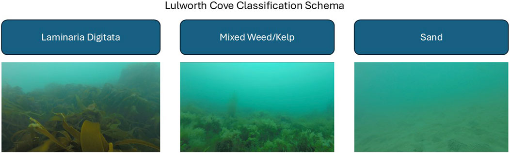
Figure 4. Classification schema. Labels and example screenshots taken from the ground truth video imagery survey.

Once classified, data was stored in a CSV file with columns labelled “x,” “y,” “class.” Due to the nature of the site, representation of classes “Laminaria Digitata” and “Sand” was lower in the ground truth dataset relative to “Mixed Weed/Kelp.” Given that imbalanced train/test datasets can lead to overfitting of the majority class (Johnson and Khoshgoftaar, 2020), random down sampling of majority classes was performed – 29 ground truth points remained. A Synthetic Minority Oversampling Technique (SMOTE) (Elreedy et al., 2024) was trialled but failed to correctly model the bed type.

Python processing

Standardisation of raster layer properties

Using bespoke code in python, several data preparation steps were performed prior to development of the classification models. Given that raster layers are stacked for data extraction at each pixel, both the extents and the resolution of each raster layer need to be identical. Spatial resolution was checked to be 0.25 m and raster layers were clipped to common spatial extents.

Next, “NoData” values were standardised. Sci-Kit’s Random Forests function does not accept the “NoData” string as a pixel value, so all no data values were converted to a placeholder integer. A standardised no data value of 9999 was chosen over 0 as some genuine values were equal to 0 (within the span bathymetry grid).

Generation of derivatives

For the bathymetry grid, the following derivatives were then generated using varying neighbourhood sizes (k = 3, 9, 15, 21, 27, 33):

• Mean

• Standard Deviation

• Slope

• Rugosity

• Curvature

• Eastness

• Northness

The same was performed for the backscatter mosaic, however only mean and standard deviation derivative layers apply. Derivatives were chosen based on their efficacy in previous studies (Porskamp et al., 2022). Derivatives were generated at different scales using SciPy’s Generic Filter module – smaller neighbourhood sizes are preferential for capturing finer details however are more susceptible to noise, larger neighbourhood sizes are resilient to noise but can lead to underfitting (Deng et al., 2023).

Segmentation and aggregation of ARA and WC layers

For the following reasons, ARA and WC layers required additional processing steps:

• ARA layers contained excess noise, likely due to failure to achieve the data acquisition targets outlined in Survey design above. Regions with reduced overlap suffer from fewer angular response comparisons

• Due to the implementation of the sidelobe filtering algorithm in Espresso, the WC mosaics suffered from narrowing swath widths and subsequent data gaps.

To combat the above, ARA and WC values were aggregated according to segments derived from the backscatter mosaic. Segmentation was performed in ArcGIS Pro, where a mean shift segmentation approach was implemented (Zhou et al., 2011). Parameters were adjusted until segments were representative of the bed’s variation at a level of detail equivalent to the desired classification resolution – spectral detail, spatial detail, and minimum segment size were set at 18, 1 and 20, respectively. For each of the ARA and WC layers, values of pixels within each segment were averaged and reassigned to all pixels within the segment. Figure 5 shows the results of the segmentation and aggregation process for WC (1–2 m) and ARA (Impedance) layers.

Figure 5

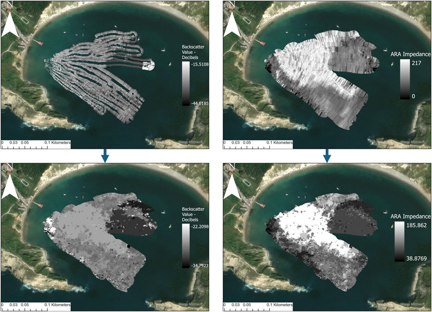
Figure 5. ARA Impedance and Water Column data before and after aggregation. Selection of maps showing the effect of aggregation of WC and ARA raster layers with respect to a segmented backscatter mosaic. To the upper left is the WC data between 1 and 2 m above the seabed in mosaic form, produced in Espresso. To the upper right is the ARA Impedance, produced in FMGT. The aggregation process was performed for a total of 5 raster layers. Maps generated in ArcGIS Pro.

Random forests algorithm

Classification models were generated using Sci-Kit’s random forests (RF) algorithm. Hyperparameters were tuned using an iterative grid search function (also from Sci-Kit) – 150 trees were found to be optimal and used for all models. A K-Folds validation method was employed, whereby data is split into distinct training and testing subsets, with prediction accuracy of the trained model informing performance metrics. Accuracy and F1-score metrics were output and evaluated for statistical significance using an ANOVA and Tukey’s HSD tests. This training and testing split is performed k number of times, with multiple rounds ensuring that the trained model is robust to different areas within the site. Given the small number of ground truth points, 3 folds (k = 3) were performed for model evaluation. A random state seed value of 42 was used for all RF executions to ensure data splits are reproducible and consistent amongst trials.

Model performance was measured using several different statistics. For each fold, the following metrics were output and averaged:

• Accuracy metric representing the percentage of successful predictions

• Precision metric representing the number of successful positive predictions over total positive predictions (successful and unsuccessful) for each class

• Recall metric representing the number of successful positive predictions over total number of positive samples (regardless of prediction success) for each class

• F1-score which is the harmonic mean of both precision and recall

In Sci-kit learn, a global feature importance measure, namely the Gini importance, was used to attribute normalised importance values to each input feature (in this case the input raster layers) (Saarela and Jauhiainen, 2021; Hapfelmeier et al., 2014). Although importance values do not come with metadata to facilitate evaluation of their trustworthiness, they do provide insight into what layers provide the best discriminatory power.

Results

From each of the data product outputs (Figure 6), common seabed patterns can be discerned. Through assessment of ground truth data, satellite imagery, and site observations these patterns appear to correlate with different seabed types. Perhaps the most clearly defined zone across all data product outputs is in the North West of the survey area, which is associated with sandy seabed. From the Bathymetry, Backscatter and ARA outputs it is possible to discern areas of dense foliage to the West/South West, as well as more sparse foliage in the North. It is difficult to discern dense foliage from sparse foliage based on the water column outputs.

Figure 6

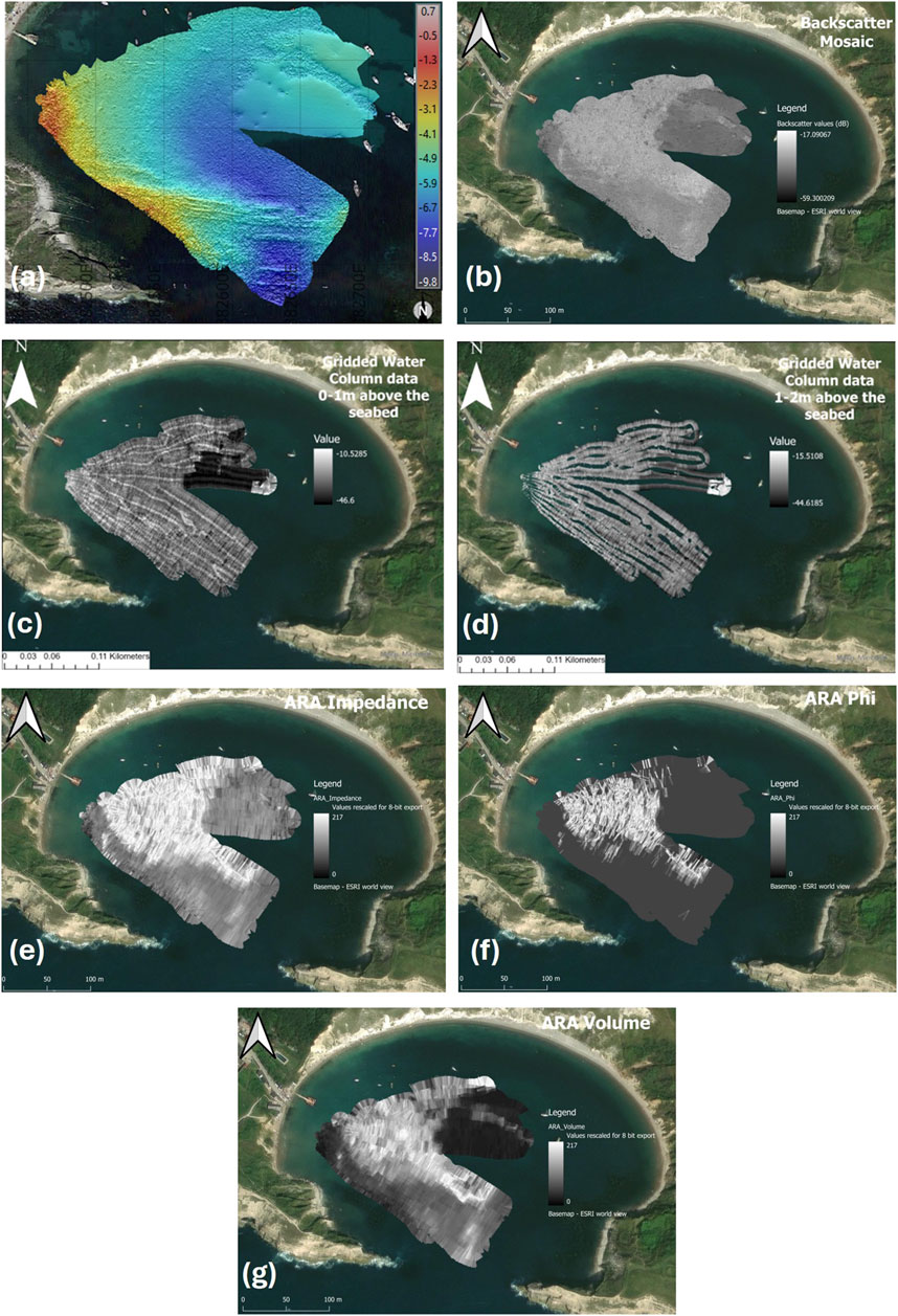
Figure 6. All data product outputs at a resolution of 0.25m. (A) Mean bathymetry (BeamworX)in metres above ODN (B) Backscatter mosaic (ArcGIS) (C) Echo integrated water column mosaic 0-1m above the seabed (ArcGIS) (D) Echo integrated water column mosaic 1–2 m above the seabed (ArcGIS) (E) ARA Impedance (QGIS) (F) ARA Phi (QGIS) (G) ARA Volume (QGIS).

Performance across data product input

Model accuracy

As shown in Figure 7, mean accuracy values ranged from 62% ± 11% (1σ) (Bathymetry) to 90% ± 10% (1σ) (All products) – error bars indicate standard deviation across folds. Mean accuracies indicate a steady increase in ability to distinguish bed types as each data product is input, with consecutive additions producing accuracy improvements of between 3%–17%.

Figure 7

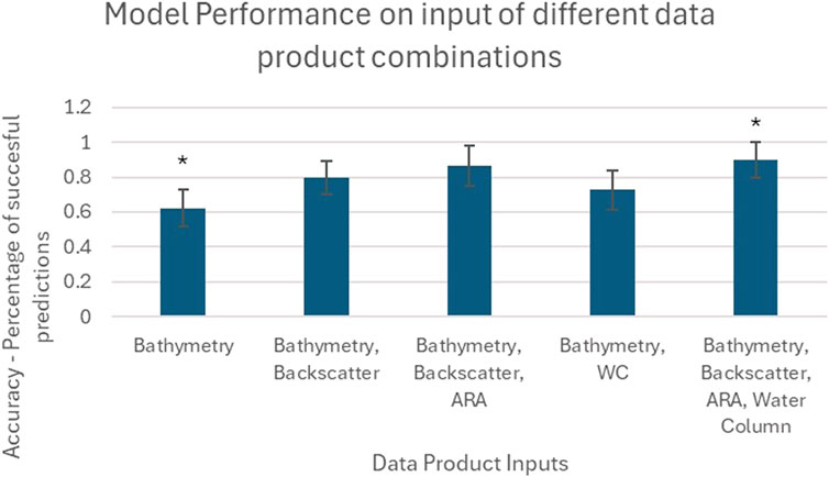
Figure 7. Mean accuracies across three folds for each of the data product combinations. Error bars indicate standard deviation, while the asterisks over Bathymetry and All Products models indicate statistical significance (at a CL of 95%).

An ANOVA test of fold accuracies for each model returned an F-statistic of 4.21 (2 d.p) and P value of 0.046 (3 d.p). The null hypothesis that all models have indifferent accuracies can therefore be rejected to a confidence level (CL) of 95%. A subsequent Tukey’s HSD test determined that a statistically significant (CL of 95%) difference in accuracy was only present between the models derived from Bathymetry and all products (Bathymetry, Backscatter, ARA, and WC) – the mean difference is 27.8% and the Tukey’s P value is 0.047 (3 d.p).

F1-score

Reporting of F1-scores provides some insight into the effect of each data product on model recall and precision for each class. Figure 8 shows F1-scores averaged over each fold, with error bars delimiting standard deviation. It appears that mixed weed/kelp is poorly predicted when the model is solely reliant on bathymetry data, scores then climb steadily as each product is incorporated. Prediction of Laminaria Digitata is relatively reliable even for the most basic model, while scores for Sand prediction jump on input of the backscatter data. Variability across folds means that none of the differences between models for each class are statistically significant (to a CL of 95%) – the Weed class is closest, with a P value of 0.156 (3 d.p). On top of this, there are no statistically significant (95% CL) differences between F1-scores of different classes within any one model – the lowest P value being 0.115 (3 d.p) for the Bathymetry model.

Figure 8

Figure 8. Class F1-scores across models. See discussion for assessment of trustworthiness.

Variable importances

Figure 9 shows the top 20 highest normalised feature importances reported after generation of the most accurate model (input of all data products).

Figure 9

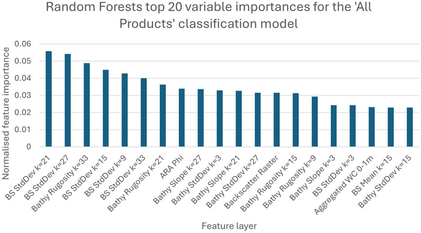
Figure 9. Top 20 variable importances for the All-Products’ classification model. See discussion for assessment of trustworthiness.

There is a clear reliance on backscatter standard deviation and bathymetry derived rugosity layers, these constitute the top 7 most important features. It is also important to note the neighbourhood scales of the most important layers – there is a disproportionate presence of the derivative layers calculated using larger k values. Of the ARA layers, only ARA Phi is included in the top 20. Only the WC layer between 0 and 1 m is included. All 61 layers were used for generation of the classifier except for mean bathymetry layers where k = 21 and k = 27, which had importance values of 0.

Smoothing improved model accuracy

As shown in Figure 10, the model input with the full range of derivatives reported higher accuracy than the one only using derivatives smoothed with a neighbourhood of size 3.

Figure 10

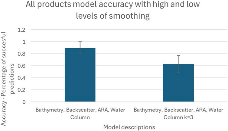
Figure 10. Plot showing the effect of differing levels of smoothing on model accuracy.

The accuracy of the model with all derivative layers was reported to be 27.5 percentage points higher than the model with the smaller neighbourhood size. A t-test was performed and produced a P value of 0.051. As this is greater than the critical value of 0.05 (for a 95% CL), the null hypothesis that the model accuracies are not significantly different can be accepted.

Classification maps

The output classification maps themselves can also be used to better understand how the model uses input layers to classify, as well as areas of higher and lower performance. While evaluation of the classification maps is qualitative, it does constitute an independent check of model performance across the entire site, rather than being limited to the ground truth sample points. Figure 11 shows a classification map for each model. All classification maps present similar distributions of each class within the survey site (dominance of Sand in the East, Mixed Weed/Kelp in the middle and Laminaria Digitata in the West). Besides some disagreement at the intersection of all three classes in the Northwest, classification maps generated by all three models except for the bathymetry only model are very similar. The bathymetry only classification map presents striations of Sand within the areas dominated by Mixed Weed/Kelp – these striations mirror the appearance of the bedrock on which the Mixed Weed/Kelp is attached.

Figure 11

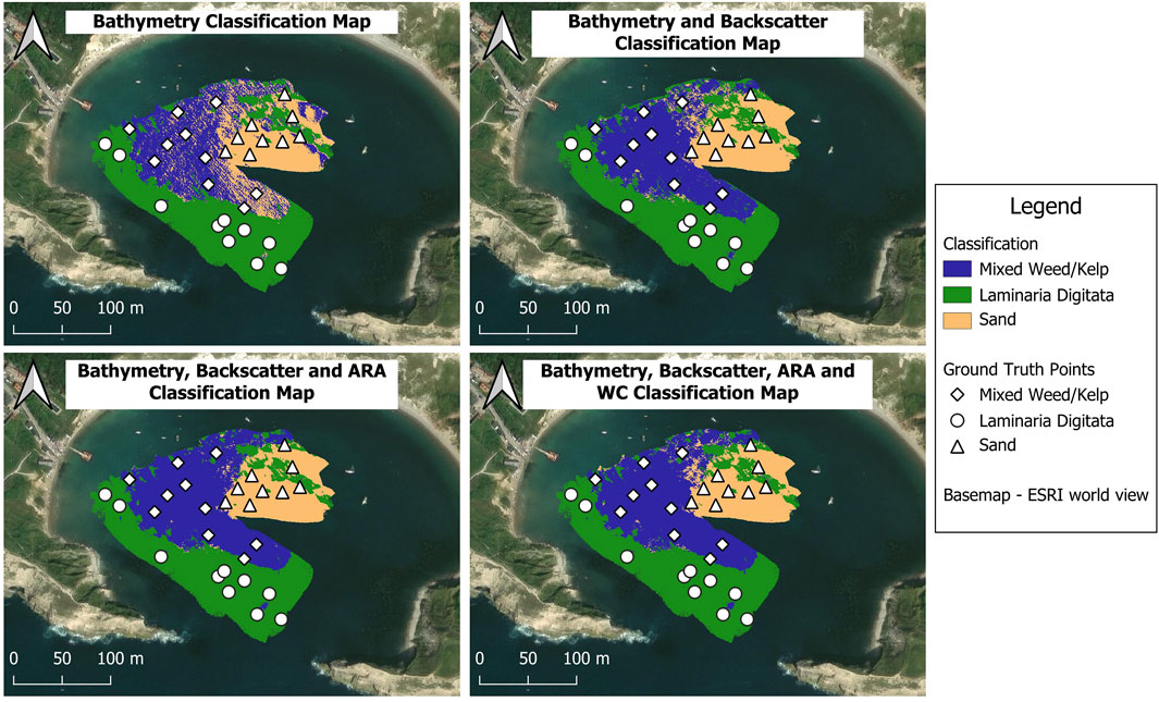
Figure 11. Classification maps representing the effect of consecutive addition of data products. Maps generated in ArcGIS Pro.

Discussion

All products classification model accuracy

When using all available MBES data products, an average of 90% ± 10% (1σ) of all test sample predictions were correct, while the class Laminaria Digitata achieved an F1-score of 89% ± 19% (1σ) (2 s.f). These scores are “good” by most image classification standards; however, the specific application of such technology will determine whether the method is fit for purpose. For monitoring projects for conservation of kelp, this method is far superior to traditional technologies such as towed cameras that feature an overreliance on observational and interpolated data, leading to overgeneralisation and therefore inaccuracy.

The study by Porskamp et al. (2022) is the only other example of previous research that considers all MBES data products for an image based classification of macroalgae. The accuracy reported for the relevant model was 67.77%, with the macroalgae class scoring 76.57%. The variations between these studies could be due to several reasons, these are discussed below.

Differing survey sites

The Porskamp, Schimel et al. (2022) study site was in Southern Australia and housed different species of kelp. Named macroalgae species observed in the ground truth survey included Seirococcus axilaris, Acrocarpia paniculata and Cystophora platylobium–the acoustic properties of these species likely differ from those found in the UK. Given that an accurate model will discriminate based on contrasting properties of the seabed, similarities amongst the bed types will make classes inherently difficult to differentiate. This is perhaps particularly pertinent in the Porskamp et al. (2022) study as there is a class containing “tall branching sponge communities” - these may bear similar characteristics with the macroalgae and therefore explain confusion between classes. The Porskamp et al. (2022) study was conducted in an open coastal environment over a much greater depth range, the greater noise and reduced data density associated with this environment may have influenced model performance.

Differing input layer resolutions

This study inputted raster layers at a horizontal resolution of 0.25 m, while Porskamp et al. (2022) used layers at a resolution of 1 m. Higher resolution could explain the greater model accuracies. The smoothing effect associated with calculating derivatives using k neighbourhoods likely results in further loss of detail and model accuracy - Porskamp et al. (2022) used greater neighbourhood sizes (up to 501). Equally, it could be that discrete areas of a single bed type within the site were smaller and therefore more prone to misclassification.

Larger classification schema

The category including brown macroalgae (kelp) was only introduced in the classification schema of the highest detail, where there were 7 other categories. By virtue of a higher number of categories, the probability of misclassification increases.

Model accuracy on addition of MBES data products

The results showed a steady increase in mean accuracy as each data product was inputted. This data serves to inform survey design for MBES kelp monitoring surveys, as the added value of incorporation of each data product can be considered against the challenges associated with their collection.

Value of bathymetry

The model generated on input of bathymetry and its derivatives achieved surprisingly good accuracy of 62.2% (±0.11%, 1σ). A study performed over similar seabed containing seagrass species in Greece reported similar results, whereby the bathymetry only model achieved an accuracy of 62.8% (Fakiris et al., 2019). The F1-scores indicated better precision and recall of the class Laminaria Digitata (F1-score of 0.785) relative to classes Mixed Kelp and Sand (F1-scores of 0.451 and 0.574, respectively). This is likely because of the dense foliage associated with the class Laminaria Digitata was classified as bottom detections, so the kelp morphology was represented in the data product. On the other hand, the Mixed Kelp class contained less dense foliage, so bottom detections may be representative of the actual seabed rather than the kelp canopy – the model’s confusion between Sand and Mixed Kelp is therefore more understandable. Also, given that the class Laminaria Digitata contains only one species, there will be less variation within the class, and characteristics will therefore be well represented at the ground truth points. On the other hand, the extensive variation of kelp species present in the Mixed Kelp class are unlikely to be well represented in the small number of training samples. Bathymetry data is logged by MBES systems as standard and provides a strong foundation prior to supplementation with other data products.

Value of backscatter intensities

On addition of the backscatter mosaic and its derivative layers, the model accuracy increased by 17.4 percentage points. Fakiris et al. (2019) also reported a significant jump after input of the MBES backscatter mosaic, with model performance increasing from 62.8% to 74.2%. F1-scores suggest that while the Laminaria Digitata class precision and recall rises slightly on addition of backscatter data, Mixed Kelp and Sand rise more significantly, by 25.1% and 28.3%, respectively. While bathymetry only considers the bottom detection points, snippets data includes samples in proximity to the bottom detection (within the snippets window). Therefore, even if the bottom detections are representative of the seabed rather than the canopy (as suggested in Value of Bathymetry), the backscatter mosaic will likely consider reflectivity of the kelp foliage (if it exists within the snippets window). The differing reflectivity of sand and kelp provide strong discriminatory power in areas that bathymetry alone could not provide. Backscatter snippets are particularly valuable in this study as features are at or near the bottom detection point, kelp species where foliage is not proximal to the seabed (such as Bull kelp) will likely not be detected. Optimal survey design for backscatter and bathymetry differs slightly, however compromises can be made without major reduction in data quality.

Value of angular range analysis

This study found that mean model accuracy increased by 7.1 percentage points on addition of ARA layers, although this increase is not statistically significant. These results are somewhat supported by those presented in Che Hasan et al. (2014) and Fakiris et al. (2019), whereby the ARA features improved classification accuracy by 5.1% and 2.4%, respectively. Che Hasan et al. (2014), however, reported ARA features to be more important than the backscatter mosaic (and its derivatives), a finding not observed during this study. The observed insignificance of the ARA features is likely at least in part due to ground truth sample size and loss of detail associated with the aggregation process, both of which are discussed in Study limitations. While ARA Impedance, Volume, and Phi were identified as the most valuable exports for a similar classification application (Porskamp et al., 2022), they are derived from the ARA mean and so may not retain across track angular resolution. The value of the ARA data may have been improved if separate layers were exported for the distinct angular ranges (nadir, near and far) (Lurton et al., 2015). To perform meaningful angular response analysis, 100% overlap is required instead of the commonly adopted 20% target for standard bathymetry survey. While increased overlap does not degrade bathymetry data (data redundancy is healthy), it will significantly increase survey time.

Value of water column data

This study found a rise of mean accuracy by 3.3% on additional input of WC data – this increase is not statistically significant; however this is likely at least in part due to validation sample size, which is discussed further in Study limitations. A marginal gain returned after addition of water column data was also observed in Porskamp et al. (2022), where model accuracy improved by 1.18%. The small increase in performance on input of WC data could be attributed to the small form of kelp present in this study – from the ground truth it was clear that all the kelp species rarely exceeded 30 cm in height, with the exception of Sea Oak (Halidrys siliquosa) which occasionally exceeded 1 m. Also, the density of kelp in some regions (western extents) meant that the canopy returns were classified as bottom detections – intensities were therefore captured by the backscatter (snippets) rather than the WC (where bottom detections were masked in processing). Efficacy of WC data is likely greater for monitoring kelp species such as bull kelp and giant kelp, where there is a greater prominence of foliage within the water column. Problems associated with the increasing data volumes attributed to improved sonar systems (wider swath, increased ping rates) are compounded when all data products are acquired. As returns and intensities are logged over increasing portions of the echogram for each beam, data volumes rise dramatically from bathymetry to backscatter (snippets) to water column. Despite compression of WC data by many systems (including the Norbit system used in this study), data storage, transfer, and processing can still become significant challenges. Although all data considered in this study was collected during a single survey, an additional survey was performed beforehand to refine configurations, collecting bathymetry and backscatter (snippets) data only. The volume of MBES data collected during the test survey totalled 6.15 GB, while collected data volume from the survey with all products (including WC) totalled 18.7 GB. It is important to note that as both backscatter and WC were collected simultaneously, the Norbit system automatically restricted WC logging to 1 in every 5 pings – logging WC data for every ping would have further increased volume. While these surveys were not identical, they were performed for approximately equal amounts of time over the same area, and so their comparison provides an indication of the effect of WC data collection on data volumes. This study was designed as a proof of concept at a scale whereby this was not problematic, however a cost-effective implementation of this technology will surely be on a larger scale; the necessity of WC data therefore must be questioned. It seems that WC data is required for optimal model performance, however improvements are small, and model performance is already strong prior to its inclusion – opting not to collect WC data could be the more cost-effective solution.

Model inaccuracies undetected by validation method

Performance metrics are based on subsets of the ground truth sampling points and serve only as an estimation of true performance. Knowledge of the site, derived from observations during acquisition, ground truth, and the MBES data itself, can serve as a means for further validation. On generating the classification maps, it was clear that a particular area had been misclassified due to presence of a mooring line – Figure 12 shows a screenshot of the point cloud as well as an indication of the area on a classification map. This misclassification examples the vulnerability of machine learning methodologies to anomalies not represented in the training data – the extension of the mooring line into the water column has obvious similarities with the Laminaria Digitata class, explaining the classification as such.

Figure 12

Figure 12. Indication of misclassification by Bathymetry and Classification map comparison. Left: Screenshot taken from Autoclean (BeamworX) shwoing bathymetry grid and an inspection area containing point data of a mooring line. Both are coloured according to height above ODN. Right: All data products classification map with a red box delimiting the extents equivalent to the inspection area in Autoclean. The mooring line has caused a misclassification.

MBES technology for high resolution kelp monitoring

Although the output classification maps are of 0.25 m resolution, the smoothing performed for generation of the derivative layers reduces the effective resolution. The variable importances suggest that in order to maximise performance, layers derived with neighbourhood sizes of 21, 27 and 33 pixels were favoured – each pixel describes the variation over a ∼5–9 m square. When minimal smoothing is performed (only derivatives of k = 3 are input), model accuracy falls from 90% (±10%, 1σ) to 62.6% (±11%, 1σ). This fall in accuracy is likely related to the training data – if resolution exceeds the positioning accuracy of the ground truth, the model will be trained and tested improperly. Also, classification of ground truth samples was performed with the positioning imprecision in mind, classes were assigned based on the properties of the local area of seabed rather than directly below the camera. As a result, the indication that accuracy suffers at high resolution (0.25 m) is likely due mostly to design of the ground truth survey rather than shortcomings of the MBES technology. While the increased data samples attributed to snippets means mosaic resolution can be high, resolution of bathymetry data often restricts the resolution of model inputs (as all layers must be of the same resolution and extents). Rate of data collection of modern MBES systems in shallow water facilitates gridding at a resolution of 0.25 m (sufficient samples are required in each pixel to improve confidence) – while more resolute grids can be produced, the increased survey time makes this costly. Even if different kelp species could be distinguished based on form and reflectivity, 0.25 m resolution is not sufficient to discriminate between single organisms within a mixed kelp bed (see Figure 13 below for a highly mixed kelp bed). As a result, some level of aggregation (as seen in the Laminaria Digitata class) is required for successful identification of a kelp species.

Figure 13

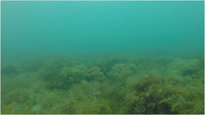
Figure 13. A screenshot of a ground truth sample containing several species of kelp in close proximity.

Study limitations

This study was designed in accordance with several constraints, some of which introduced limitations.

Sub optimal navigation tracks

As discussed in the methodology, the study site was chosen for its known presence of kelp as well as its sheltered waters to suit the survey platform. Due to the high occurrence of obstacles within the cove and poor navigational control of the survey vessel, motion artefacts accrued within the backscatter mosaic (despite post processing of position and motion data) – reasons for this are discussed in the Survey design. The effect of the sub-optimal navigation on predictive accuracy is difficult to quantify however is likely to be minimal given most of the site characterised by flat seabed (Lurton et al., 2018).

Lack of ground truth samples for training and testing

Lack of training samples reduces the ability of the Random Forests algorithm to derive relationships between classes and extracted features, while lack of testing samples reduces the ability to confidently evaluate the model. The lack of samples relates to the disproportionality of class presence (by area) within the site, large areas were classed as Mixed Weed/Kelp. This disproportionality was then reflected in the ground truth dataset, with the classes Laminaria Digitata, Mixed Weed/Kelp and Sand represented by 61, 18 and 13 samples, respectively. For sites of complex class distribution, synthetic up-sampling techniques are unreliable; down-sampling of majority classes is therefore the only way to prevent imbalance and overfitting. Although ground truth samples could be made at a higher density, this could introduce effects of spatial autocorrelation, whereby the RF algorithm learns to what extent homogeneous classes aggregate in space, leading to geographical variables (X, Y) being used to improve prediction – this introduces overestimation of model accuracy and poor predictive performance on unseen data (Griffith and Chun, 2014).

Loss of detail associated with the segmentation and aggregation process

The approach taken when dealing with missing values has been shown to have a significant impact on Machine Learning derived models (Hasan et al., 2021). The poor spatial coverage of the ARA and WC data relative to the bathymetry and backscatter warranted the reliance on a different approach to dealing with missing values. While the segmentation and aggregation method used in this study improves spatial coverage, it also involves averaging large amounts of data – this inevitably removes much of the detail within these datasets. As well as this, the segmentation was performed using the backscatter dataset – by averaging over segments produced based on a different dataset, the patterns inherent to the ARA and WC datasets may be lost or skewed.

Positional accuracy of ground truth data

While GNSS observables were post processed to achieve sub-decimetric precision, layback of the weighted rope introduces additional error. While this error is difficult to quantify given it is highly dependent on depth, current and speed of rope release, it is estimated to be up to 1 m. Given that a model cannot accurately resolve beyond the resolution of its training data, this constitutes a significant limitation. Layback could be mitigated by use of a telescopic pole instead of rope (significant practical challenges) or incorporation of SONAR based positioning such as Ultra Short Base Line (USBL) (high expense).

Identification of kelp species from ground truthing imagery

Kelp was identified and subsequently classified based on morphological characteristics. As some kelp species appear similar to the untrained eye, ground truth samples may in some instances suffer from misclassification. Figure 13 examples this ambiguity.

Correlation of input variables

Naturally, input layers are highly correlated, especially given that many are derived from the same data. Although correlated variables are known to cause overfitting for many machine learning algorithms, Random Forests (as well as other decision tree algorithms) are known to be robust to multicollinearity (Grömping, 2009; Dormann et al., 2013). Despite this, it is noted that collinearity can have an impact on variable importance scores, making them unreliable. With more time, this study would have benefitted from some form of iterative feature selection procedure to mitigate this problem.

Software provision

The novel WC processing software Espresso is the first to produce WC mosaics, an exciting development when considering image classification methodologies for benthic monitoring. Despite this, the current version does not support some functions common to other MBES processing software.

• A post processed trajectory (such as Applanix’s SBET) cannot be applied. A reliance on the live trajectory is particularly damaging in this study given that only satellite based DGNSS corrections were received and applied (resulting in GNSS accuracies in the order of tens of centimetres)

• Sound velocity corrections cannot be applied

Opportunities for integration with present survey campaigns

MBES technology has become standard for the majority of subsea survey applications. As accessibility and capability of hardware improves, there has been an occurrence of exponential growth in data acquired both within the UK and globally. Emergence of USVs is expected to compound this growth as well as improve coverage in otherwise uncharted territories. Organisations such as the UKHO commission regular surveys for safety of navigation, while the huge volume of engineering works in the energy and communications sectors demands frequent near shore surveys. The regularity and often iterative nature of these MBES surveys paired with their presence in near shore regions makes for potentially valuable data with regards to kelp forest monitoring. This study shows that acquisition of multiple data products, collected with minimal deviation from standard bathymetric survey design, can be leveraged to distinguish kelp species; although the challenge of coordination is significant there is clear opportunity to exploit existing survey infrastructure to derive valuable kelp distribution data as a biproduct, which will form the foundation of kelp forest conservation efforts.

Conclusion and recommendations

While considering other technologies, this study has demonstrated the applicability of MBES systems for monitoring kelp species common to the UK coastline, with models achieving mean accuracy scores as high as 90% (±10%, 1σ). The classification schema used demonstrates the ability to distinguish a single kelp species from areas of mixed kelp (provided it is sufficiently aggregated) – F1-score for the class Laminaria Digitata was 0.889 (3 d.p). Distinction of kelp species is of interest given the range of different environmental services they provide. Features such as capacity for improved spatial and temporal resolution relative to satellite imagery as well as superior coverage relative to camera surveys likely outweigh the costs associated with hardware, software, and training. When considering MBES data products, bathymetry, backscatter (including ARA) and water column all improved discriminatory power. Bathymetry and backscatter were highly valuable and introduce fewer trade-offs while ARA and WC products introduced less impressive model accuracy improvements and challenges with survey design and data volumes, respectively. The primary limitation of this study was that, by virtue of a small study area, amount of training and testing data was reduced, leading to reduced confidence in model performance metrics.

Future research could work to improve confidence in observed results, as well as explore the effect of factors such as frequency on predictive power. Novel analysis of multispectral multibeam data associated with benthic habitats has indicated that a range of frequencies expose additional differences between seabed types – with high and low frequencies delivering improved differentiation of fine reef/seagrass texture and more course sediments, respectively (Schulze et al., 2022; Menandro et al., 2024). The applicability of this multispectral approach to kelp monitoring in the UK is currently untested. Also, incorporation of signal-based processing approaches (demonstrated by Kruss et al. (2019) and Che Hasan et al. (2014)) with the image based approach used in this study could reap benefits in the form of improved classification and biomass estimations. This study focusses on the ability to distinguish Laminaria Digitata from mixed kelp species, however the extent to which other species can be discerned is another area for future research. As potential performance of this technology is clarified, a requirement for effective implementation strategies will emerge, benthic survey as a biproduct of engineering and safety of navigation surveys could be a method to reduce costs.

Data availability statement

The datasets presented in this article are not readily available because Sharing of data requires expressed permission from Lulworth Estate. Permission has been granted for publication. Requests to access the datasets should be directed to amFrZWJlcnJ5MjVAb3V0bG9vay5jb20=.

Author contributions

JB: Conceptualization, Data curation, Formal Analysis, Investigation, Methodology, Project administration, Validation, Visualization, Writing–original draft, Writing–review and editing. CN: Funding acquisition, Project administration, Resources, Software, Supervision, Writing–original draft, Writing–review and editing.

Funding

The author(s) declare that no financial support was received for the research, authorship, and/or publication of this article.

Acknowledgments

The support I’ve received throughout this project is greatly appreciated. Massive thanks to: CN for her supervision and advice throughout. The Port of London Authority for affording me the resources required for data collection. Dr Chris Yesson from the Zoological Society of London as well as members of IFCA and the SKRP for helping find a suitable study site. Lulworth Estate for granting permissions to acquire data at Lulworth Cove. JP Cheminade of Geodesea and BeamworX for provision of software as well as guidance through acquisition. QPS for provision of the QPS software suite. LandScope Engineering for assistance with post processing of ground truthing positions. Aleksandra Kruss of Norbit for advice regarding multibeam configurations. Alexandre Schimel for guidance with Espresso Software – special thanks for uploading an updated software version after my data exposed a bug. Friends and family for lending time and equipment during ground truth data acquisition – Martin Berry and Robert Slomczynski.

Conflict of interest

The authors declare that the research was conducted in the absence of any commercial or financial relationships that could be construed as a potential conflict of interest.

Generative AI statement

The author(s) declare that no Generative AI was used in the creation of this manuscript.

Publisher’s note

All claims expressed in this article are solely those of the authors and do not necessarily represent those of their affiliated organizations, or those of the publisher, the editors and the reviewers. Any product that may be evaluated in this article, or claim that may be made by its manufacturer, is not guaranteed or endorsed by the publisher.

References

Alam, A., Bhat, M. S., and Maheen, M. (2020). Using Landsat satellite data for assessing the land use and land cover change in Kashmir valley. GeoJournal 85, 1529–1543. doi:10.1007/s10708-019-10037-x

CrossRef Full Text | Google Scholar

Butchart, S. H. M., Walpole, M., Collen, B., Van Strien, A., Scharlemann, J. P. W., Almond, R. E. A., et al. (2010). Global biodiversity: indicators of recent declines. Science 328, 1164–1168. doi:10.1126/science.1187512

PubMed Abstract | CrossRef Full Text | Google Scholar

Che Hasan, R., Ierodiaconou, D., Laurenson, L., and Schimel, A. (2014). Integrating multibeam backscatter angular response, mosaic and bathymetry data for benthic habitat mapping. PLOS ONE 9, e97339. doi:10.1371/journal.pone.0097339

PubMed Abstract | CrossRef Full Text | Google Scholar

Deng, S., Wang, L., Guan, S., Li, M., and Wang, L. (2023). Non-parametric nearest neighbor classification based on global variance difference. Int. J. Comput. Intell. Syst. 16, 26. doi:10.1007/s44196-023-00200-1

CrossRef Full Text | Google Scholar

Dormann, C., Elith, J., Bacher, S., Buchmann, C., Carl, G., Carré, G., et al. (2013). Collinearity: a review of methods to deal with it and a simulation study evaluating their performance. Ecography 36, 27–46. doi:10.1111/j.1600-0587.2012.07348.x

CrossRef Full Text | Google Scholar

Eger, A. M., Marzinelli, E. M., Beas-Luna, R., Blain, C. O., Blamey, L. K., Byrnes, J. E. K., et al. (2023). The value of ecosystem services in global marine kelp forests. Nat. Commun. 14, 1894. doi:10.1038/s41467-023-37385-0

PubMed Abstract | CrossRef Full Text | Google Scholar

Eger, A., Aguirre, J. D., Altamirano, M., Arafeh-Dalmau, N., Arroyo, N. L., Bauer-Civiello, A. M., et al. (2024). The Kelp Forest Challenge: a collaborative global movement to protect and restore 4 million hectares of kelp forests. J. Appl. Phycol. 36, 951–964. doi:10.1007/s10811-023-03103-y

CrossRef Full Text | Google Scholar

Elreedy, D., Atiya, A. F., and Kamalov, F. (2024). A theoretical distribution analysis of synthetic minority oversampling technique (SMOTE) for imbalanced learning. Mach. Learn. 113, 4903–4923. doi:10.1007/s10994-022-06296-4

CrossRef Full Text | Google Scholar

Fakiris, E., Blondel, P., Papatheodorou, G., Christodoulou, D., Dimas, X., Georgiou, N., et al. (2019). Multi-frequency, multi-sonar mapping of shallow habitats—efficacy and management implications in the national marine park of zakynthos, Greece. Remote Sens. 11, 461. doi:10.3390/rs11040461

CrossRef Full Text | Google Scholar

Filbee-Dexter, K., Pessarrodona, A., Pedersen, M. F., Wernberg, T., Duarte, C. M., Assis, J., et al. (2024). Carbon export from seaweed forests to deep ocean sinks. Nat. Geosci. 17, 552–559. doi:10.1038/s41561-024-01449-7

CrossRef Full Text | Google Scholar

Gendall, L., Schroeder, S. B., Wills, P., Hessing-Lewis, M., and Costa, M. (2023). A multi-satellite mapping framework for floating kelp forests. Remote Sens. 15, 1276. doi:10.3390/rs15051276

CrossRef Full Text | Google Scholar

Gong, X., Zhang, R., and Fang, J. (2013). Application of unscented R–T–S smoothing on INS/GPS integration system post processing for airborne earth observation. Measurement 46, 1074–1083. doi:10.1016/j.measurement.2012.11.028

CrossRef Full Text | Google Scholar

Griffith, D., and Chun, Y. (2014). “Spatial autocorrelation and spatial filtering,” in Handbook of regional science. Editors M. M. Fischer,, and P. Nijkamp (Berlin, Heidelberg: Springer Berlin Heidelberg).

CrossRef Full Text | Google Scholar

Grömping, U. (2009). Variable importance assessment in regression: linear regression versus random forest. Am. Statistician 63, 308–319. doi:10.1198/tast.2009.08199

CrossRef Full Text | Google Scholar

Hapfelmeier, A., Hothorn, T., Ulm, K., and Strobl, C. (2014). A new variable importance measure for random forests with missing data. Statistics Comput. 24, 21–34. doi:10.1007/s11222-012-9349-1

CrossRef Full Text | Google Scholar

Hasan, M. K., Alam, M. A., Roy, S., Dutta, A., Jawad, M. T., and Das, S. (2021). Missing value imputation affects the performance of machine learning: a review and analysis of the literature (2010–2021). Inf. Med. Unlocked 27, 100799. doi:10.1016/j.imu.2021.100799

CrossRef Full Text | Google Scholar

Jackson, D. R., Winebrenner, D. P., and Ishimaru, A. (1986). Application of the composite roughness model to high-frequency bottom backscattering. J. Acoust. Soc. Am. 79, 1410–1422. doi:10.1121/1.393669

CrossRef Full Text | Google Scholar

Johnson, J. M., and Khoshgoftaar, T. M. (2020). The effects of data sampling with deep learning and highly imbalanced big data. Inf. Syst. Front. 22, 1113–1131. doi:10.1007/s10796-020-10022-7

CrossRef Full Text | Google Scholar

Koehl, M. A. R. (1984). How do benthic organisms withstand moving Water?1. Am. Zoologist 24, 57–70. doi:10.1093/icb/24.1.57

CrossRef Full Text | Google Scholar

Kruss, A., Wiktor, J., Wiktor, J., and Tatarek, A. (2019). “Acoustic detection of macroalgae in a dynamic Arctic environment (Isfjorden, West Spitsbergen) using multibeam echosounder,”in 2019 IEEE Underwater Technology (UT), Kaohsiung, Taiwan, April 16–19, 2019, 1–7. doi:10.1109/ut.2019.8734323

CrossRef Full Text | Google Scholar

Lamarche, G., and Lurton, X. (2018). Recommendations for improved and coherent acquisition and processing of backscatter data from seafloor-mapping sonars. Mar. Geophys. Res. 39, 5–22. doi:10.1007/s11001-017-9315-6

CrossRef Full Text | Google Scholar

Liu, C.-C., Chen, Y.-H., Wu, M.-H. M., Wei, C., and Ko, M.-H. (2019). Assessment of forest restoration with multitemporal remote sensing imagery. Sci. Rep. 9, 7279. doi:10.1038/s41598-019-43544-5

PubMed Abstract | CrossRef Full Text | Google Scholar

Lurton, X., Eleftherakis, D., and Augustin, J.-M. (2018). Analysis of seafloor backscatter strength dependence on the survey azimuth using multibeam echosounder data. Mar. Geophys. Res. 39, 183–203. doi:10.1007/s11001-017-9318-3

CrossRef Full Text | Google Scholar

Lurton, X., Lamarche, G., Brown, C., Lucieer, V., Rice, G., Schimel, A., et al. (2015). Backscatter measurements by seafloor-mapping sonars - guidelines and Recommendations. Available at: http://geohab.org/wp-content/uploads/2014/05/BSWG-REPORT-MAY2015.pdf (Accessed August 5, 2024).

Google Scholar

Menandro, P. S., Vieira, F. V., Bastos, A. C., and Brown, C. J. (2024). Exploring the multispectral acoustic response of reef habitats. Front. Remote Sens. 5. doi:10.3389/frsen.2024.1490741

CrossRef Full Text | Google Scholar

Morris, R. L., Graham, T. D. J., Kelvin, J., Ghisalberti, M., and Swearer, S. E. (2020). Kelp beds as coastal protection: wave attenuation of Ecklonia radiata in a shallow coastal bay. Ann. Bot. 125, 235–246. doi:10.1093/aob/mcz127

PubMed Abstract | CrossRef Full Text | Google Scholar

Norbit (2024). TN-140075-20 Sonar User Manual. Trondheim, Norway: NORBIT Subsea AS. Available at: https://norbit.com/subsea (Accessed February 12, 2025).

Google Scholar

Overrein, M. M., Tinn, P., Aldridge, D., Johnsen, G., and Fragoso, G. M. (2024). Biomass estimations of cultivated kelp using underwater RGB images from a mini-ROV and computer vision approaches. Front. Mar. Sci. 11. doi:10.3389/fmars.2024.1324075

CrossRef Full Text | Google Scholar

Porskamp, P., Schimel, A., Young, M., Rattray, A., Ladroit, Y., and Ierodiaconou, D. (2022). Integrating multibeam echosounder water-column data into benthic habitat mapping. Limnol. Oceanogr. 67, 1701–1713. doi:10.1002/lno.12160

CrossRef Full Text | Google Scholar

Pouliquen, E., and Lyons, A. P. (2002). Backscattering from bioturbated sediments at very high frequency. IEEE J. Ocean. Eng. 27, 388–402. doi:10.1109/joe.2002.1040926

CrossRef Full Text | Google Scholar

Saarela, M., and Jauhiainen, S. (2021). Comparison of feature importance measures as explanations for classification models. SN Appl. Sci. 3, 272. doi:10.1007/s42452-021-04148-9

CrossRef Full Text | Google Scholar

Sabirova, A., Rassabin, M., Fedorenko, R., and Afanasyev, I. (2019). “Ground profile recovery from aerial 3D LiDAR-based maps,”in 2019 24th Conference of Open Innovations Association (FRUCT), Moscow, Russia, 367–374. doi:10.23919/FRUCT.2019.8711928

CrossRef Full Text | Google Scholar

Schimel, A. C. G., Brown, C. J., and Ierodiaconou, D. (2020). Automated filtering of multibeam water-column data to detect relative abundance of giant kelp (macrocystis pyrifera). Remote Sens. 12, 1371. doi:10.3390/rs12091371

CrossRef Full Text | Google Scholar

Schulze, I., Gogina, M., Schönke, M., Zettler, M. L., and Feldens, P. (2022). Seasonal change of multifrequency backscatter in three Baltic Sea habitats. Front. Remote Sens. 3. doi:10.3389/frsen.2022.956994

CrossRef Full Text | Google Scholar

St-Pierre, A. P., and Gagnon, P. (2020). Kelp-bed dynamics across scales: enhancing mapping capability with remote sensing and GIS. J. Exp. Mar. Biol. Ecol. 522, 151246. doi:10.1016/j.jembe.2019.151246

CrossRef Full Text | Google Scholar

Townsend, M., Davies, K., Hanley, N., Hewitt, J. E., Lundquist, C. J., and Lohrer, A. M. (2018). The challenge of implementing the marine ecosystem service concept. Front. Mar. Sci. 5. doi:10.3389/fmars.2018.00359

CrossRef Full Text | Google Scholar

Turco, F., Ladroit, Y., Watson, S. J., Seabrook, S., Law, C. S., Crutchley, G. J., et al. (2022). Estimates of methane release from gas seeps at the southern hikurangi margin, New Zealand. Front. Earth Sci. 10. doi:10.3389/feart.2022.834047

PubMed Abstract | CrossRef Full Text | Google Scholar

Umanzor, S., and Stephens, T. (2023). Nitrogen and carbon removal capacity by farmed kelp alaria marginata and saccharina latissima varies by species. Aquac. J. 3, 1–6. doi:10.3390/aquacj3010001

CrossRef Full Text | Google Scholar

Wear, B., O'Connor, N. E., Schmid, M. J., and Jackson, M. C. (2023). What does the future look like for kelp when facing multiple stressors? Ecol. Evol. 13, e10203. doi:10.1002/ece3.10203

PubMed Abstract | CrossRef Full Text | Google Scholar

Wernberg, T., Krumhansl, K., Filbee-Dexter, K., and Pedersen, M. F. (2019). “Chapter 3 - status and trends for the world’s kelp forests,” in World seas: an environmental evaluation. 2nd Edn, Editor C. SHEPPARD (Academic Press).

Google Scholar

Wulder, M. A., Hermosilla, T., White, J. C., Bater, C. W., Hobart, G., and Bronson, S. C. (2024). Development and implementation of a stand-level satellite-based forest inventory for Canada. For. An Int. J. For. Res. 97, 546–563. doi:10.1093/forestry/cpad065

CrossRef Full Text | Google Scholar

Zhou, H., Wang, X., and Schaefer, G. (2011). “Mean shift and its application in image segmentation,” in Innovations in intelligent image analysis. Editors H. Kwaśnicka,, and L. C. Jain (Berlin, Heidelberg: Springer Berlin Heidelberg).

CrossRef Full Text | Google Scholar