Mixture density networks for re-constructing historical ocean-color products over inland and coastal waters: demonstration and validation

Ocean color remote sensing tracks water quality globally, but multispectral ocean color sensors often struggle with complex coastal and inland waters. Traditional models have difficulty capturing detailed relationships between remote sensing reflectance (R_rs), biogeochemical properties (BPs), and inherent optical properties (IOPs) in these complex water bodies. We developed a robust Mixture Density Network (MDN) model to retrieve 10 relevant biogeochemical and optical variables from heritage multispectral ocean color missions. These variables include chlorophyll-a (Chla) and total suspended solids (TSS), as well as the absorbing components of IOPs at their reference wavelengths. The heritage missions include the Moderate Resolution Imaging Spectroradiometer (MODIS) aboard Aqua and Terra, the Environmental Satellite (Envisat) Medium Resolution Imaging Spectrometer (MERIS), and the Visible Infrared Imaging Radiometer Suite (VIIRS) onboard the Suomi National Polar-orbiting Partnership (Suomi NPP). Our model is trained and tested on all available in situ spectra from an augmented version of the GLObal Reflectance community dataset for Imaging and optical sensing of Aquatic environments (GLORIA) (N = 9,956) after having added globally distributed in situ IOP measurements. Our model is validated on satellite match-ups corresponding to the SeaWiFS Bio-optical Archive and Storage System (SeaBASS) database. For both training and validation, the hyperspectral in situ radiometric and absorption datasets were resampled via the relative spectral response functions of MODIS, MERIS, and VIIRS to simulate the response of each multispectral ocean color mission. Using hold-out (80–20 split) and leave-one-out testing methods, the retrieved parameters exhibited variable uncertainty represented by the Median Symmetric Residual (MdSR) for each parameter and sensor combination. The median MdSR over all 10 variables for the hold-out testing method was 25.9%, 24.5%, and 28.9% for MODIS, MERIS, and VIIRS, respectively. TSS was the parameter with the highest MdSR for all three sensors (MODIS, VIIRS, and MERIS). The developed MDN was applied to satellite-derived R_rs products to practically validate their quality via the SeaBASS dataset. The median MdSR from all estimated variables for each sensor from the matchup analysis is 63.21% for MODIS/A, 63.15% for MODIS/T, 60.45% for MERIS, and 75.19% for VIIRS. We found that the MDN model is sensitive to the instrument noise and uncertainties from atmospheric correction present in multispectral satellite-derived R_rs. The overall performance of the MDN model presented here was also analyzed qualitatively for near-simultaneous images of MODIS/A and VIIRS as well as MODIS/T and MERIS to understand and demonstrate the product resemblance and discrepancies in retrieved variables. The developed MDN is shown to be capable of robustly retrieving 10 water quality variables for monitoring coastal and inland waters from multiple multispectral satellite sensors (MODIS, MERIS, and VIIRS).

1 Introduction

Coastal and inland waters are the most affected by changes in environmental conditions, industrial development, or human intervention, leading to an increase in dissolved and suspended particles like phytoplankton, sediments, and colored dissolved organic matter in the water column (Stumpf et al., 2012; Brown et al., 2015; Pick, 2016; Binding et al., 2021; Jane et al., 2021). Gradually, the interaction of these dissolved and suspended particles with the aquatic environment leads to major changes in biogeochemical parameters (BPs) such as chlorophyll-a (Chla), total suspended solids (TSS), and colored dissolved organic matter (cdom), which subsequently affects the water quality as well as visibility within the water column (Babin et al., 2003). Managing the water quality of inland and coastal waters poses a challenge due to anthropogenic activities, eutrophication, and climate change. Monitoring the water quality for these aquatic ecosystems is essential for sustainable water resource management, providing the foundation on which it is based (Bartram and Ballance, 1996). However, tracking long-term changes in BPs through ship-based measurements poses significant challenges and expenses.

Over the past 25 years, freely available multispectral radiometric images from a series of multispectral ocean color satellite sensors have compiled a vast global observational database of remote sensing reflectance (McClain, 2009). These sensors, deployed on various platforms, include the Environmental satellite (Envisat) Medium Resolution Imaging Spectrometer (MERIS) spanning from 2003 to 2011, the Moderate Resolution Imaging Spectroradiometer (MODIS) aboard Terra (since 1999) and Aqua (since 2002), as well as the Visible Infrared Imaging Radiometer Suite (VIIRS) on the Suomi National Polar-orbiting Partnership (Suomi NPP, since 2011). These heritage sensors, some of which are still operational at the time of writing, have unequivocally broadened our awareness and comprehension of ocean and coastal ecosystems (Cao et al., 2022).

Central to aquatic remote sensing is the concept of apparent and inherent optical properties (AOPs and IOPs, respectively). IOPs include the spectral absorption and scattering properties of water and its constituents (Gordon et al., 1975). The spectral shape of the total absorption coefficient depends on both water and the BPs. The absorbing IOPs can be further divided as a function of these constituents (Werdell et al., 2018). The absorption and scattering coefficients depend solely on the medium or water column properties and are not influenced by the geometry of the light field (Werdell et al., 2018). Moreover, the absorption by BPs is typically close to zero at near-infrared (NIR) wavelengths, making NIR wavelengths indirectly useful for removing atmospheric interference in satellite-captured images (Bailey et al., 2010), unless in very turbid waters. The optically relevant BPs and IOPs can be estimated from the measured multispectral remote sensing reflectance ($R_{rs}\left(\lambda \right)$), an AOP obtained after the radiometric, geometric, and atmospheric correction of top-of-atmosphere (TOA) satellite measured radiance (Gordon and Wang, 1994). This quantity, $R_{rs}$ (=$L_w$/ $E_d$), is defined as the ratio of water-leaving radiance ($L_w$) and downwelling irradiance ($E_d$) evaluated just above the water (Mobley, 1999). The spectral shape and magnitude of the $R_{rs}$ are highly sensitive to the processes of absorption and scattering (IOPs) by optically relevant BPs in the water while being relatively insensitive to changes in the ambient light field (IOCCG, 2008; IOCCG, 2009; IOCCG, 2014), making $R_{rs}$ suitable for retrieving the IOPs.

Numerous remote sensing algorithms exist for quantifying BPs and IOPs from $R_{rs}$ captured using ocean color satellite sensors over oceanic and coastal waters. Empirical algorithms primarily rely on single-band linear relationships or multi-band $R_{rs}$ ratios for estimating BPs, such as Chla (O’Reilly et al., 1998; O’Reilly and Werdell, 2019) and TSS (Nechad et al., 2010; Ondrusek et al., 2012; Novoa et al., 2017). The spectra of absorbing IOPs are estimated using exponential functions with the required input parameters, such as absorption coefficients and corresponding slopes of phytoplankton - $a_{ph}$ (Sosik and Mitchell, 1995; Babin et al., 2003; Bricaud et al., 2004; Devred et al., 2022; Wei et al., 2023), non-algal particles - $a_{nap}$ (Bowers and Binding, 2006), and colored dissolved organic matter - $a_{cdom}$ (Binding et al., 2008; Shanmugam, 2011; Mannino et al., 2014) at their reference wavelengths. The slopes are obtained from multi-band $R_{rs}$ ratios or functions of BPs. However, these algorithms require substantial datasets to calibrate the underlying models and are primarily applicable to the specific water type for which the model is calibrated. Outside of empirical algorithms, IOPs are estimated using inversion algorithms grounded in statistical modeling, such as Garver Siegel Maritorena – GSM model (Maritorena et al., 2002), Generalised IOP - GIOP model (Werdell et al., 2013) and Linear Matrix Inversion - LMI algorithm (Hoge and Lyon, 1996), utilizing semi-analytical methodologies and prior knowledge of BPs (Wang et al., 2017). Semi-analytical algorithms primarily utilize $R_{rs}$ to deduce IOPs and subsequently estimate BPs by integrating empirical parameters and bio-optical models. Furthermore, the quasi-analytical algorithm - QAA, widely employed over the past decade, represents another prevalent model for IOP inversion (Lee et al., 2002; McKinna et al., 2015; Montes-Hugo and Xie, 2015).

Advanced machine learning models show promise for non-unique inverse problems, such as retrieving BPs and IOPs from R_rs. One such approach is using Bayesian neural networks (BNNs) (Werther et al., 2022). BNNs can retrieve water quality parameters from satellite imagery and have been validated using satellite data. Another proven machine learning method entails using mixture density networks (MDNs) and has been leveraged for the estimation of both BPs and IOPs (O’Shea et al., 2023). MDNs address non-unique inverse problems, like inferring BPs from $R_{rs}$, by modeling the output as a probability distribution over possible output values. Therefore, the distribution is modeled using a mixture of Gaussians (Bishop, 1994; 1995). Instead of providing the average value of the expected output distribution, like typical multilayer perceptrons (MLPs), MDN provides the full output distribution, enabling the user to study the distribution and choose an appropriate output value, enhancing the overall estimation when the predicted output distribution is multimodal or asymmetric. Further, since the MDNs and BNNs predict output distributions, these distributions can also be used to model the confidence in a specific prediction (Saranathan et al., 2023; Werther et al., 2022) enabling users to disregard predictions on data outside of the training dataset’s range. Specialized MDNs have been developed to estimate specific water quality indicators, BPs and IOPs, such as Secchi disk depth (Maciel et al., 2023), Chla (Pahlevan et al., 2020; 2021b; Smith et al., 2021), TSS (Balasubramanian et al., 2020), phycocyanin (O’Shea et al., 2021; Fickas et al., 2023), and $a_{ph}$ (Pahlevan et al., 2021b) from both multispectral and hyperspectral satellite data, applicable to inland and coastal waters. Furthermore, this architecture has been effectively utilized to concurrently estimate two BPs and an IOP at a single wavelength [Chla, TSS, and a_cdom (440)] (Pahlevan et al., 2022) and tested with multispectral satellite sensor datasets, such as from the Multispectral Instrument (MSI) and Ocean and Land Colour Instrument (OLCI) onboard Sentinel-2, and Sentinel-3, respectively. Recently, the model has been effectively applied for hyperspectral remote sensing by estimating BPs (Chla, TSS, PC) and hyperspectral IOPs ($a_{ph}$, $a_{nap}$, and $a_{cdom}$) and tested with satellite data from the Hyperspectral Imager for the Coastal Ocean (HICO) and PRecursore IperSpettrale della Missione Applicativa (PRISMA) missions (O’Shea et al., 2023; Lima et al., 2023), indicating its potential application to the recently launched Ocean Color Instrument (OCI) of the Plankton, Aerosol, Cloud, ocean Ecosystem (PACE) mission. In general, due to their demonstrated effectiveness in the non-unique inverse estimation of BPs and IOPs, along with their inherent capacity to gauge uncertainties, MDNs are highly suitable for concurrently retrieving various BPs and IOPs for scientific and water quality management applications.

Daily satellite visits offer a wealth of information crucial for retrospective analysis, particularly in the realm of multispectral ocean color data, which can be effectively used for studying climate change and biogeochemical modeling (Behrenfeld et al., 2006; Platt and Sathyendranath, 2008; Stramski, 2008; Hu et al., 2010; Wang et al., 2011). MODIS has been providing long-term ocean color data since its mission began (1999-), shortly followed by MERIS sensor (2002-). After MERIS’s operational lifeended (2012), the ongoing VIIRS sensor (2011-) continued to provide ocean colordata together with MODIS (Lai et al., 2023). Accurately assessing and quantifying uncertainties in satellite ocean color products is crucial, making thorough validation a challenging task for ocean color missions (Hooker and McClain, 2000). Since these are long-term satellites, there is a possibility of sensor performance degradation (Hu and Le, 2014; Cao et al., 2018). Therefore, regular calibration using the Marine Optical Buoy [MOBY (Clark et al., 1997; Wang et al., 2015)] dataset and validation using the Aerosol Robotic Network - Ocean Color component [AERONET-OC (Zibordi et al., 2006; Mélin et al., 2007)] dataset are essential for these ocean color sensors and have been conducted in several studies (Cannizzaro et al., 2019; Garcia et al., 2020; Pahlevan et al., 2021a). Validations of BPs (Werdell et al., 2009; Cui et al., 2010; Odermatt et al., 2010; Tilstone et al., 2012) and IOPs (Delgado et al., 2019; Fan et al., 2021; Huan et al., 2021) through ocean color imagery have been conducted over regional waters, including ocean, coastal, and inland waters. The consistency of data products from algorithms simultaneously predicting AOPs from multiple satellite missions has been evaluated over different ocean and coastal regions (Cui et al., 2014; Cao et al., 2018; Barnes et al., 2019). Over inland waters, various factors such as the need for atmospheric correction in a more challenging atmosphere due to complex aerosol compositions (compared to oceanic aerosols) and compensation for adjacency effects from nearby lands, produce significantly higher uncertainty for remote sensing (Liu et al., 2024), and data products from multimission datasets have not yet been formally assessed for consistency (Cao et al., 2018; Cao et al., 2023; Pahlevan et al., 2024). A comprehensive assessment that encompasses a wider range of factors, ensuring the reliability and applicability of satellite-derived ocean color data on a global scale, especially for coastal and inland water ecosystems is urgently needed.

The multimission ocean color satellite dataset, along with the extensive hyperspectral field observations from the augmented GLORIA and SeaBASS databases, provides crucial support for analyzing performance of multimission sensor products in both nearshore and inland waters. This study aims at developing a technique based on MDNs for retrieving 10 water quality variables including two BPs and three IOPs at reference bands over coastal and inland waters. The outline of this manuscript is as follows. In Section 2, we discuss the general techniques for obtaining IOPs from ocean color R_rs. Section 3 explains the details of the augmented GLORIA and SeaBASS in situ datasets and the four ocean color satellite sensor datasets used for estimating the 10 BP and IOP variables. Section 4 explains the deep learning method used for the estimation of these water quality parameters from $R_{rs}$ of the four heritage ocean color sensors. Section 5 explains the validation of the developed model with the in situ dataset and multimission ocean color sensor dataset encompassing MODIS/A, MODIS/T, MERIS and VIIRS. In addition to the validation results, the spatial data analysis covers water quality parameters using the near simultaneous measurements of the aforementioned ocean color sensors. Section 6 describes the spatial data analysis. The results are discussed in Section 7, and the study is summarized in Section 8.

2 Background

In general, R_rs derived from satellite data, can be estimated from the normalized water-leaving radiance (nL_w) by dividing it by the constant mean extraterrestrial solar irradiance (F₀). This R_rs is associated with other AOPs, which depend on the ambient light field and water constituents, as well as IOPs. Enhancing the relationship between $R_{rs}$ and IOPs in natural waters is fundamental for the accurate estimation of waters constituents from radiometric observations. For this, R_rs can be converted to subsurface remote sensing reflectance r_rs using a relationship (Equation 1) provided as (Lee et al., 2002):

$r_{rs}\left(\lambda \right)=\left(\frac{R_{rs}\left(\lambda \right)}{0.52+1.7R_{rs}\left(\lambda \right)}\right)(1)$

Here, r_rs does not have the effect of the sun being off-zenith associated with it (Werdell et al., 2018). The simplified correspondence between $r_{rs}$ and IOPs revolves around absorption ($a$) and backscattering ($b_b$) coefficients, with g representing a complex function dependent on several factors including wavelength, solar angle, wind speed, and water optical properties, given as Equation 2 (Gordon et al., 1988):

$r_{rs}\left(\lambda \right)=g\left(\lambda \right)\times \left(\frac{b_b\left(\lambda \right)}{a\left(\lambda \right)+b_b\left(\lambda \right)}\right)(2)$

Quantifying the fraction of incident light absorbed within the water column per unit distance, absorption coefficients encompass contributions from pure water $\left(a_w\right)$, phytoplankton $\left(a_{ph}\right)$, non-algal particles $\left(a_{nap}\right)$, and colored dissolved organic matter $\left(a_{cdom}\right)$. The combined absorption by non-algal particles (a_nap, also denoted as a_d) and colored dissolved organic matter ($a_{cdom}$, also known as a_g) can be referred to as a_dg. The total absorption coefficient (unit: m⁻¹) can be expressed as Equation 3:

$a\left(\lambda \right)=a_w\left(\lambda \right)+a_{ph}\left(\lambda \right)+a_{cdom}\left(\lambda \right)+a_{nap}\left(\lambda \right)(3)$

In clear oceanic conditions (Case 1), a parametrization function can effectively relate Chla to total particulate absorption due to minimal contributions from non-algal particles. However, in coastal and inland waters (Case 2), variations in components like phytoplankton, suspended solids, and colored dissolved organic matter may occur independently from Chla, leading to diverse spectral signatures of R_rs.

The $a_{ph}$ has been related to Chla and phytoplankton biomass (Binding et al., 2008) and can be determined by multiplying their specific absorption coefficients with the concentration of Chla (Roesler and Perry, 1995), as follows:

$a_{ph}\left(\lambda \right)=a_{ph}^{*}\times Chla(4)$

Here, $a_{ph}^{*}$ in Equation 4 is the phytoplankton-specific absorption coefficient, defined per unit concentration of Chla, that varies widely depending on phytoplankton species composition (Bricaud et al., 1995).

The absorption coefficient for colored dissolved organic matter (see Equation 5) typically follows an exponential decrease as wavelength increases in the near-UV and visible spectral regions, and is observed as (Bricaud et al., 1981):

$a_{cdom}\left(\lambda \right)=a_{cdom}\left({\lambda }_0\right)\times {\mathit{exp}}^{-S\times \left({\lambda -\lambda }_0\right)}(5)$

Here, $a_{cdom}({\lambda }_0$) denotes the absorption coefficient at the reference wavelength ${\lambda }_0$ (Brezonik et al., 2015). The value of $a_{cdom}({\lambda }_0$) is often utilized to characterize the colored dissolved organic matter concentration in a specific water body. Additionally, the spectral slope S (nm⁻¹), which remains independent of ${\lambda }_0$, signifies the rate at which absorption decreases with increasing wavelength.

The last absorption component, non-algal particles $\left(a_{nap}\right)$, generally consists of non-algal organic detritus, living non-algal particles and suspended sediments (Binding et al., 2008). Further, the $a_{nap}\left(\lambda \right)$ decreases exponentially with increasing wavelength and the general (Equation 6) is as follows (Roesler et al., 1989; Bricaud et al., 1998; Binding et al., 2008):

$a_{nap}\left(\lambda \right)=a_{nap}\left({\lambda }_0\right)\times {\mathit{exp}}^{-S\times \left({\lambda -\lambda }_0\right)}(6)$

Here, $a_{nap}$ at reference wavelength ${\lambda }_0$ and slope S can be estimated as a function of TSS concentration using an empirical relationship (Babin et al., 2003).

Another IOP is the backscattering coefficient (b_b), which is typically expressed using two backscattering components (Equation 7): pure water backscattering (b_bw) and particulate backscattering (b_bp). The wavelength dependence of b_b is expressed as follows:

$b_b\left(\lambda \right)=b_{bw}\left(\lambda \right)+b_{bp}\left(555\right){\left(\frac{555}{\lambda }\right)}^Y(7)$

Here, the values of b_bw are derived from laboratory measurements (Morel, 1974). The b_bp component is influenced by particles in seawater, such as minerals, phytoplankton, and organic matter (Vaillancourt et al., 2004; Woźniak et al., 2019). Y represents the spectral slope of b_bp. Y and b_bp at a reference wavelength of 555 nm can be estimated from R_rs(λ). Most studies use these general (Equations 1–7) to retrieve IOPs from R_rs (Maritorena et al., 2002; Lee et al., 2002; Werdell et al., 2013).

3 Dataset

3.1 Training dataset: GLORIA

Our model training dataset utilizes the co-located measurements of hyperspectral $R_{rs}$ and constituent concentration data from the GLObal Reflectance community dataset for Imaging and optical sensing of Aquatic environments (GLORIA) (Lehmann et al., 2023). This dataset is complemented with co-located hyperspectral inherent optical properties (IOPs), including absorption coefficients for phytoplankton (a_ph), non-algal particles (a_nap), and colored dissolved organic matter (a_cdom) (O’Shea et al., 2023).

The GLORIA dataset is further enhanced with additional co-located measurements of hyperspectral R_rs, IOPs, and BPs sourced from individual contributors and compiled datasets included in our augmented GLORIA dataset. Other than GLORIA (N = 7572), 2384 samples of $R_{rs}$ with at least one corresponding BP or IOP were incorporated to create the augmented GLORIA dataset (N = 9956). These 2384 samples are obtained from the SeaBASS repository (Marra et al., 1988; Carder, 1997; 1998; Carder and Kirkpatrick, 1998; Carder and Mitchell, 1999; Cota and Zimmerman, 2000; Stumpf, 2001; Carder and Hu, 2005; Hill and Zimmerman, 2010; Hu and Muller-Karger, 2012; Muller-Karger, 2015), PANGAEA repository (Garaba et al., 2011; Knaeps et al., 2018; Gonçalves-Araujo et al., 2018; Casey et al., 2020; Lavigne et al., 2022), and other publications (Brewin et al., 2023; Burket et al., 2023; Simis et al., 2023). Datasets from other coastal and inland regions such as Indonesian waters, the North Sea, Estonian waters, Lake Taihu, Lake Erie, California Bay, Curonian Lagoon, and Lake Xingyun comprise additional parts of the augmented GLORIA. The locations of the hyperspectral IOP measurements corresponding to those in the augmented GLORIA dataset, are shown in Figure 1 and representing coastal and inland waters of various countries around the globe. Most of these BPs and IOPs have been previously documented in various publications, each providing maps of individual parameters by region (Balasubramanian et al., 2020; Jiang et al., 2021; O’Shea et al., 2021; Smith et al., 2021; Pahlevan et al., 2021b; 2022).

Figure 1

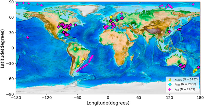
Figure 1. The geographical distribution of the hyperspectral IOPs (a_cdom, a_nap and a_ph) in the augmented GLORIA dataset, used for model development.

Figure 2 shows the frequency distributions of the BP/IOP/R_rs values in the training dataset. There are 6153 samples for Chla (with mean of 36 mg m⁻³ and median of 6.8 mg m⁻³), 5358 for TSS (with mean of 28.9 g m⁻³ and median of 9.5 g m⁻³), 3757 for a_cdom at 443 nm (with mean of 1.1 m⁻¹ and median of 0.58 m⁻¹), 2988 for a_nap at 443 nm (with mean of 0.51 m⁻¹ and median of 0.16 m⁻¹), and 2903 for a_ph at 443 nm (with mean of 0.71 m⁻¹ and median of 0.16 m⁻¹), paired with 9956 total R_rs. Additional details about the dataset are provided in Table 1. The compiled dataset provides a comprehensive perspective on global aquatic environments, serving as the training and testing dataset for this study.

Figure 2

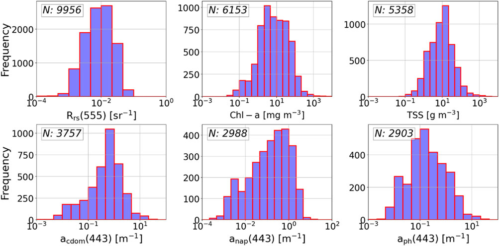
Figure 2. Frequency distributions of in situ hyperspectral remote sensing reflectance $R_{rs}$, with BPs (Chla and TSS) and hyperspectral IOPs (a_cdom, a_nap and a_ph), used as the training and testing dataset (N = 9,956) for model development.

Table 1

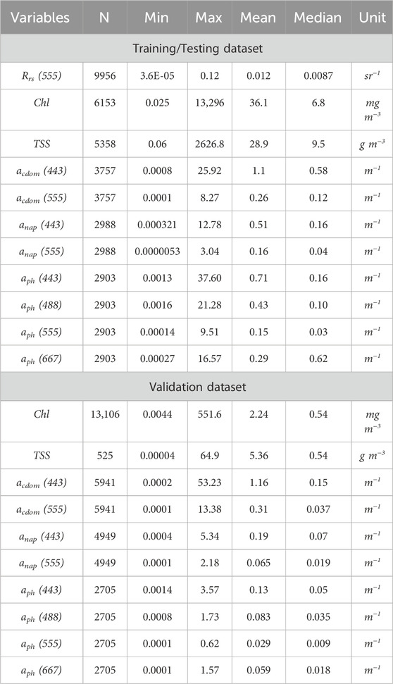
Table 1. Overview of the training Data from the augmented GLORIA dataset and the validation data from the SeaBASS database.

3.2 Validation dataset: SeaBASS

The validation dataset for this study is obtained from the NASA SeaBASS repository (Werdell and Bailey, 2005). Although the SeaBASS repository (https://seabass.gsfc.nasa.gov/) contains various ocean color parameters, we specifically acquired data for parameters such as BPs (Chla and TSS) and hyperspectral IOPs (a_cdom, a_nap and a_ph), which are limited to this study. Some SeaBASS data has been integrated into GLORIA to support model training (Section 3.1). To prevent duplication, only SeaBASS data lacking R_rs has been acquired for the validation dataset, ensuring its independence from the GLORIA dataset. The geographical locations of these BPs and hyperspectral IOPs are shown in Figure 3. This dataset includes information from 55 principal investigators (PIs) (refer to Supplementary Appendix Table SB1 for the list of PIs) representing different institutions and countries, covering global coastal, inland, and open ocean waters. The acquired data span almost 25 years, from 1994 to 2019.

Figure 3

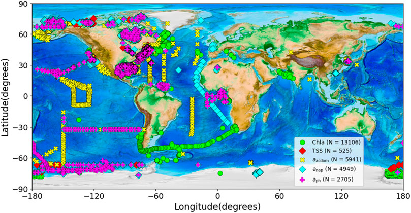
Figure 3. The geographical distribution of the BPs (Chla and TSS) and hyperspectral IOPs (a_cdom, a_nap and a_ph) in the datasets extracted from the SeaBASS database (from 1994 to 2019) used for model validation.

Figure 4 shows the frequency distributions of the validation dataset acquired from the SeaBASS database. There are 13,106 samples for Chla (with mean of 2.24 mg m⁻³ and median of 0.54 mg m⁻³), 525 for TSS (with mean of 5.36 g m⁻³ and median of 0.54 g m⁻³), 5941 for a_cdom at 443 nm (with mean of 1.16 m⁻¹ and median of 0.15 m⁻¹), 4949 for a_nap at 443 nm (with mean of 0.195 m⁻¹ and median of 0.07 m⁻¹), and 2705 for a_ph at 443 nm (with mean of 0.13 m⁻¹ and median of 0.05 m⁻¹). More information about the validation dataset is presented in Table 1.

Figure 4

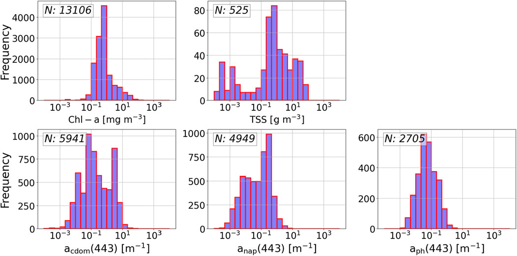
Figure 4. Frequency distributions of in situ BPs (Chla and TSS) and hyperspectral IOPs (a_cdom, a_nap and a_ph) from the SeaBASS database used as the satellite-ground matchup samples for model validation.

3.3 Multispectral ocean color imagery

The satellite datasets used in this study include MODIS/Terra (1999–present) and MODIS/Aqua (2002–present), each with 11 spectral bands; MERIS (2002–2012) with 11 bands; and VIIRS (2011–present) with 6 bands. A detailed summary of these sensors is provided in Table 2. Satellite images covering the date and location of each validation data point are Level-1A observations sourced from the NASA Goddard Space Flight Center (GSFC) repository (https://oceancolor.nasa.gsfc.gov). These L1A images were processed using NASA’s SeaWiFS Data Analysis System (SeaDAS v7.5.3). In this process, atmospheric correction was performed using NIR-SWIR band combinations: 869/2130 nm for MODIS/Terra and MODIS/Aqua, and 862/2257 nm for VIIRS. For MERIS, which lacks SWIR bands, atmospheric correction utilized a two-band NIR combination (779/865 nm). The SeaDAS output includes the Level-2 products encompassing R_rs at different bands.

Table 2

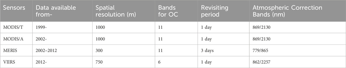
Table 2. Details of the four different ocean color sensors and the atmospheric correction bands used for R_rs retrievals in this study. Details of the atmospheric correction process are provided in Section 4.5.

4 Methodology

This section elaborates on the detailed methodology utilized in this study for extracting BPs and IOPs from three ocean color missions, as depicted in Figure 5. The approach integrates a MDN to construct a robust deep learning model. To build the model, we employed the augmented GLORIA dataset integrated with IOPs for training and testing purposes. For model evaluation, we utilized a matchup dataset sourced from three different sensors: MODIS, MERIS, and VIIRS, aligned with corresponding SeaBASS datasets. This section presents a detailed overview of the MDN model development and the procedures for processing satellite images.

Figure 5

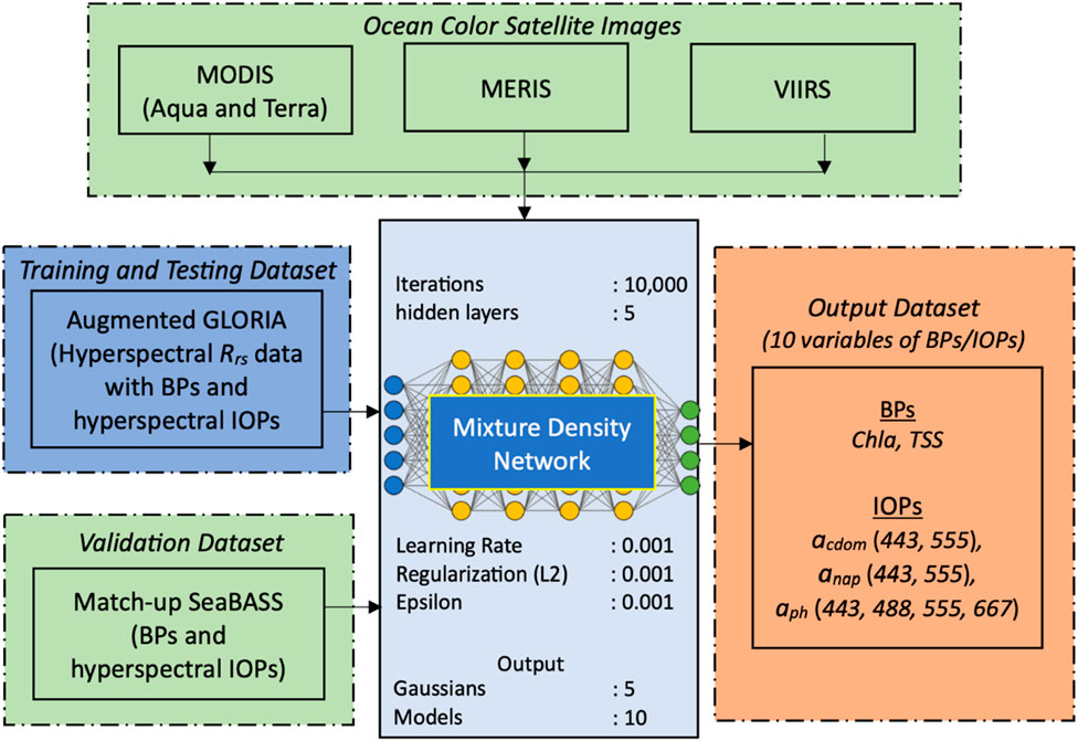
Figure 5. Schematic block diagram showing the dataset used in the development of the MDN model for the inversion of BPs and IOPs for multimission ocean color sensors.

4.1 Mixture density network features

In this study, MDNs are utilized to predict the target variables. Traditional machine learning models like MLPs or other empirical models typically yield a single estimate for the output variable without providing insights into the distribution of estimates, or possible multimodality in the output distributions. Conventional neural networks directly predict target variables by approximating the conditional average of target data. However, when approximating continuous target variables (e.g., Chla or a_ph), the conditional average often falls short of representing the full statistical properties of the target space, leading to impractical solutions (Bishop, 1994).

In general, multi-parameter inversion algorithms for BPs and IOPs (Kallio et al., 2001) are expected to constrain the solution possibilities given the covariances among parameters of interest in a natural environment. This study leverages this characteristic to estimate optically relevant BPs and IOPs through MDNs. MDNs differ from traditional neural networks (Bishop, 1995; Bricaud et al., 2007; Jamet et al., 2012) by approximating the likelihoods of generated estimates as mixture of Gaussians (Bishop, 1994), thereby accommodating multimodal target distributions, a fundamental characteristic of inverse problems where a non-unique relationship exists between input and output features. MDNs offer a distinct approach by modeling conditional probabilities of the target variables based on input data, and thus, acquiring a comprehensive understanding of the probability distribution within the target space. By inherently capturing covariances among the output features, MDNs intuitively enhance accuracy compared to models focused solely on retrieving individual parameters. As output, MDNs generate the parameters of a mixture of Gaussian (MoG) distributions, i.e., a mean vector (μ), a covariance matrix (σ), and a mixing coefficient (α) corresponding to each component in the MoG.

The MDN implemented in this study follows the standard architecture for the retrieval of individual BPs (Pahlevan et al., 2020; Smith et al., 2021) and simultaneous retrieval of multiple BPs and IOPs (Pahlevan et al., 2022; O’Shea et al., 2023). Using the relative spectral response functions of the corresponding sensors, we converted hyperspectral $R_{rs}$ and IOP data obtained from the augmented GLORIA into multispectral format. We specifically selected $R_{rs}$ data within the wavelength range of 400–750 nm, covering the visible spectrum, to capture features essential for estimating BPs and IOPs, as suggested in prior studies (O’Shea et al., 2021; Pahlevan et al., 2022). We deliberately avoided higher wavelengths to mitigate interference from oxygen-A bands and atmospheric effects during correction processes. This ensemble of multispectral $R_{rs}$ and IOPs along with BPs from the augmented GLORIA is subsequently split into 80% for training the MDN model and 20% for testing it, via a hold-out approach. The hold-out approach inherently gives the model regional knowledge of estimating BPs and IOPs from R_rs as well as knowledge of the data providers collection methodologies and their associated uncertainties, essentially providing an error estimate for measurements from within the training dataset’s distribution. Also, to ensure that the model is exposed to a wide variety of R_rs we use a dynamic imputation method similar to the prior MDN approaches (Smith et al., 2021). Each sensor - MODIS, MERIS, and VIIRS - comprises distinct bands (11 for MODIS, 11 for MERIS, and 6 for VIIRS), and therefore, we trained each sensor’s model separately.

The basic MDN architecture takes the spectral remote sensing reflectance of the specific sensor as input. Band ratios (BRs) and line heights (LHs) are added to this input (O’Shea et al., 2023). The Rrs, BRs and LHs are then normalized (scaled between −1 and 1) and run through the standard weights of a neural network. The neural network uses the rectified linear unit (ReLU) activation function and negative loss likelihood loss function to update the weights (Pahlevan et al., 2020; Smith et al., 2021; O’Shea et al., 2023; Saranathan et al., 2023). The models also use a l2-weight regularization with a penalty of 0.001 on each hidden layer as mentioned in the Figure 5.

The MDN’s final layer estimates a mixture of five Gaussians, each characterized by its own statistical parameters μ_n, σ_n, and ⍺_n. These Gaussians are fed into a combination function, which generates a point estimate as the mean of the gaussian component with the largest weight in the predicted distribution. The model generates simultaneous outputs for each BP (Chla and TSS) and IOPs including a_ph at four different wavelengths (440 nm, 488 nm, 555 nm, and 670 nm), and a_cdom and a_nap at two different wavelengths (440 nm and 555 nm). Utilizing the probabilities assigned to each prediction, users have the flexibility to opt for either the maximum likelihood estimate (i.e., the prediction with the highest probability), the weighted average of all predictions, or the approximation mentioned above. This methodology mirrors established practices in prior literature. The model’s input and output features revolve around in situ $R_{rs}$ and 10 water quality variables, specifically BPs and IOPs, aligning with similar approaches documented in previous studies.

4.2 Hyperparameters

Brief experiments were conducted in previous studies (Pahlevan et al., 2020; Smith et al., 2021) to assess the potential improvement of MDN retrievals from hyperparameters. We adopted the default hyperparameters, such as regularization and learning rate, network size, and depth, from the previous work (O’Shea et al., 2023; Pahlevan et al., 2022). The details of the hyperparameters are shown in Figure 5.

4.3 Imputation

To simultaneously generate 10 different variables of BPs and IOPs, the MDN model underwent modifications to address the issue of missing samples. Not all BPs and IOPs were measured simultaneously in situ at each site. For example, of 9956 total $R_{rs}$ samples, the in situ dataset includes 6153 for Chla and 5358 for TSS. Availability drops further for IOPs such as a_cdom with 3757 samples, a_nap with 2988, and a_ph with 2903 (shown in Figure 2). To make use of the remaining 80% of the data with missing values, multiple imputation (Rubin, 2004) is utilized, drawing values from the dataset’s distribution. This method has been successfully applied for the simultaneous estimation of three BPs from multispectral satellite datasets (Pahlevan et al., 2022), assuming either Missing Completely At Random (MCAR) or, slightly weaker, Missing At Random (MAR) scenarios. In multiple imputation, m values are randomly selected from the distribution of the input dataset for the missing parameter. Rather than naively drawing from the input dataset’s distribution, MDNs enable learning the joint probability distribution of all target parameters and drawing from the learned posterior probability. This inherent capability of MDNs allows for handling Missing Not At Random (MNAR) variables, thereby improving the accuracy of imputed samples during training (Ghahramani and Jordan, 1995; Buuren and Groothuis-Oudshoorn, 2010; Galimard et al., 2018). With additional training, the accuracy of the multiple imputation method improves as the MDN better learns to represent the joint probability distribution of the target parameters. From this, multiple imputation with MDNs offers more accurate filling of missing data, resulting in a larger dataset that is available for training and potentially improved generalization.

4.4 Regional leave-one-out cross-validation

As an alternative to the hold-out assessment (Section 4.1) which estimated performance on within distribution data, the regional leave-one-out cross-validation assesses the models’ expected retrieval accuracies on out-of-distribution data. By excluding data from one region at a time during training, the regional leave-one-out cross-validation provides the model with no information on retrieving specific IOPs or BPs from R_rs at each specific region or on the uncertainties in the in situ data associated with the collection methodologies of each data provider. The GLORIA dataset, which is used primarily for model training, consists of measurements from different water types acquired by varying groups with differing measurement procedures. In spite of the collaborative community efforts, it is not clear if the training dataset captures the universal distribution for these parameters. For a clearer sense of the model performance across different water types, we perform leave-one-out type cross validation tests to provide users with a more comprehensive perspective on how the model performance extends to previously unknown dataset. For this evaluation, subset regions were identified as individual contributors/regional datasets with more than 100 samples. Following this we iteratively trained models such that for each model one regional subset was removed from the augmented GLORIA. The left-out-dataset is then used as the validation dataset for the specific model as used to evaluate the ability of these models to generalize performance for the left-out datasets. This approach is similar to experiments performed in recent studies by O’shea et al. (2023) and Saranathan et al. (2024); see Supplementary Appendix Table SB2 for details on the regional subsets. This enables a more robust comparison of the MDN accuracy across different ocean color sensors, while also estimating uncertainty across various optically distinct water bodies. By omitting entire datasets, this region-based evaluation method also addresses uncertainties stemming from differences in sampling methods and instrumentation across labs, which can impact product estimation accuracy. However, this approach encounters challenges, such as specific datasets spanning multiple regions or containing a disproportionately high number of samples for specific parameters, which impact the interpretation of the error metrics. While most datasets were assessed by region (not all samples include latitude and longitude), some datasets cover multiple regions, such as some of the SeaBASS datasets embedded in the GLORIA dataset, which cover global waters (in Supplementary Appendix Table B2). Nevertheless, this provides the added advantage of testing our algorithm with data from diverse sources (Pahlevan et al., 2022; O’Shea et al., 2023). Overall, the regional leave-one-out cross-validation assessment offers a more accurate evaluation of the model’s generalized performance on previously unseen in situ data from global coastal and inland waters analyzed at various laboratories.

4.5 Satellite image processing procedures: (AC method and matchups)

Satellite images sourced from MODIS/A, MODIS/T, MERIS, and VIIRS, covering the date and location of each validation data point, are Level-1A observations from the NASA Goddard Space Flight Center (GSFC) repository (https://oceancolor.nasa.gsfc.gov). These images underwent processing using NASA’s SeaWiFS Data Analysis System (SeaDAS v7.5.3) software, employing a standard iterative atmospheric correction procedure (Gordon and Wang, 1994), with different NIR/SWIR band combinations specific to each sensor (details in Section 3.2). This correction aimed to remove atmospheric interference from the TOA signal. Following atmospheric correction, the $R_{rs}$ products underwent further processing using 3 × 3 pixel windows, with the sampling point location designated as the center pixel. Only windows with a valid count of more than 5 pixels were considered for computation. The median $R_{rs}$ value from the 9 (3 × 3) pixels, co-located on the same day within +/− 3 h of the sampling time, was utilized for validation purposes. Other scenarios in the matchup analysis, such as the coefficient of variation (cv < 0.2) and turbidity flag, are not considered in this study due to the limited number of matchups from the available datasets.

Although the pixel sizes of MERIS and VIIRS differ significantly from that of MODIS, this study focuses solely on assessing the performance of each ocean color sensor over inland and coastal waters. Since no intercomparison between the sensors is conducted, there is no attempt to match the MERIS and VIIRS pixels with those of MODIS in this study. The retrieved $R_{rs}$ data consisted of 11 bands (at wavelengths of 412, 443, 469, 488, 531, 551, 555, 645, 667, 678, and 748 nm) from MODIS, 11 bands (at wavelengths of 412, 443, 490, 510, 560, 620, 665, 681, 708, 754, and 761 nm) from MERIS, and 6 bands (at wavelengths of 410, 443, 486, 551, 671, and 745 nm) from VIIRS. These data served as inputs for the MDN model for the estimation of BPs and IOPs.

4.6 Performance metrics

To evaluate the performance of MDN-derived ocean color products (BPs and IOPs) obtained from three distinct sensors, we conduct an evaluation employing standard statistical methods. This includes the utilization of logarithmically transformed metrics.

The log-transformed metrics includes the Median Symmetric Residual (MdSR, ε) and Signed Symmetric Percentage Bias (SSPB, β), which are suitable for data that spans orders of magnitude, symmetric, easy to interpret, and resistant to outliers and bad data (Morley et al., 2018), rendering them ideal for assessing uncertainty when working with large water quality datasets. These two primary metrics are expressed as follows:

$\epsilon =100\times \left(e^{\left(median\left(\left|\mathit{log}\left(E_i/M_i\right)\right|\right)\right.})-1\right)(8)$

$\beta =100\times sign\left(MR\right)\times \left(e^{\left|MR\right|}-1\right)(9)$

Here, MR - Median Ratio represents the median of the logarithmic ratio between estimated and measured variables. The MdSR can be interpreted as the unsigned percentage error with perfect accuracy achieved at 0% whereas the SSPB can be interpreted as a mean percentage error with perfect bias achieved at 0%, positive values indicating overestimation and negative indicating underestimation. Additionally, other log-transformed metrics such as root mean square log-error (RMSLE) are employed for the evaluation analysis. The metrics are computed in log-space for a better assessment of the algorithms owing to the log-normal distribution of the BP data. These metrics represent the ones utilized in Morley et al. (2018) with slight modifications for enhanced interpretability and robustness.

5 Results

The MDN architecture achieves low median retrieval errors (<45%) for all 10 variables of BPs and IOPs from in situ R_rs. The test results on 20% of the in situ augmented GLORIA samples are shown in the Appendix (refer to Supplementary Appendix Figures SA1-A3, and performance metrics in Supplementary Appendix Tables SB3-B6) at the spectral resolutions of the MODIS, MERIS, and VIIRS sensors. This prior analysis facilitates the evaluation of the model’s performance with satellite datasets through matchup analysis and the results of the leave-one-out cross-validation are discussed in the following sub-sections.

5.1 Satellite data validation

Previous studies have thoroughly analyzed MDN performance and compared it with leading models, utilizing resampled GLORIA R_rs for various sensors such as OLI, MSI, OLCI, HICO, and PRISMA (Pahlevan et al., 2022; O’Shea et al., 2023) and validated atmospheric correction results for MODIS/T, MODIS/A, MERIS, and VIIRS (Pahlevan et al., 2024). That said it is also essential to measure the practical performance of the models and we, therefore, test the models using MODIS/T, MODIS/A, MERIS, and VIIRS data through matchup analysis using the SeaBASS dataset, as depicted in Figures 6–9. The geographical distribution of the SeaBASS matchups (+/−3 h) with their year-wise distribution for these ocean color missions are shown in the appendix (Supplementary Appendix Figures SA4, A5). The matchups for Chla, TSS, a_cdom, a_nap, and a_ph encompass wide ranges, indicating comprehensive dataset utilization across coastal and inland waters. Given the varying quantities of data across different variables and sensors, direct comparisons among multiple sensors are not pursued. Instead, the focus lies on elucidating each sensor’s performance regarding the retrieval of variables from $R_{rs}$. Given the extensive prior comparisons with standard models in the published literature, this results section primarily concentrates on MDN retrieval accuracy from different ocean color sensors using the SeaBASS validation dataset.

Figure 6

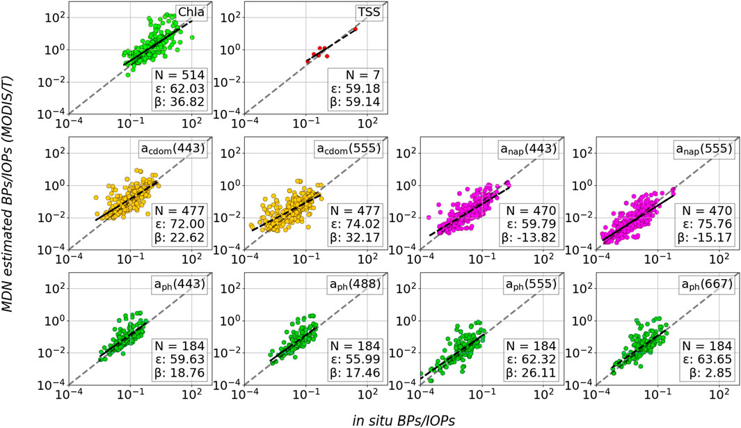
Figure 6. Scatter plots for comparison between MDN-estimated BPs/IOPs from MODIS/T satellite imagery and in situ measured BPs/IOPs from the SeaBASS dataset using co-located satellite-ground matchup samples. Satellite sampling times are matched with in situ sample collection times with a time interval within +/−3 h.

Figure 6 depicts the in situ BPs and IOPs plotted against their MDN-estimated counterparts from MODIS/T data. The dataset comprises at least 470 matchups for variables like Chla, a_cdom, and a_nap, 184 matchups for a_ph, and a considerably smaller number (7) for TSS. Notably, the ε reveals varying performance across the variables. Specifically, for a_ph, ε stands notably lower than 60% in the blue bands and higher than 62% in the green and red bands. a_cdom stands out with an ε value of greater than 72%. Conversely, a_nap demonstrates higher accuracy, with an ε ranging from 59% to 76%. The ε values of BPs such as Chla and TSS are 62% and 59%, respectively. Examining β, we observe that a_ph maintains a low range (<30%), indicating relatively balanced estimates. The β values for a_cdom are higher than those of a_ph, while a_nap exhibits significantly lower negative values. Additionally, β values for Chla and TSS indicate notable overestimation at 37% and 59%, respectively. These findings underscore the variability in accuracy and bias across the assessed variables, highlighting areas for further investigation and potential refinement in modeling approaches.

Figure 7 compares MDN-estimated variables derived from MODIS/A data against in situ BPs and IOPs. Comparable numbers of samples were obtained from MODIS/T (Figure 6) and MODIS/A matchup analyses. Notably, ε is considerably higher for a_nap, ranging from 84% to 87% for MODIS/A. Conversely, errors for variables such as Chla, TSS and a_ph fall within the low range of 43%–62% and errors for a_cdom within the slightly higher range of 71%–88%. A notable observation is the proficient retrieval of Chla and a_ph across four different bands. The β for a_cdom remains very low, ranging from 1% to 5%. Conversely, the β for a_nap displays predominantly negative values (−23% to −25%), indicating underestimation in the retrievals. Although Chla exhibits a positive bias, registering an overestimation of 44%, a_ph displays bias (β) values of 28%–36%, except at 667 nm with 14%. These results suggest that the overall retrieval performance is satisfactory.

Figure 7

Figure 7. Scatter plots for comparison between MDN-estimated BPs/IOPs from MODIS/A satellite imagery and in situ measured BPs/IOPs from the SeaBASS dataset using co-located satellite-ground matchup samples. Satellite sampling times are matched with in situ sample collection times with a time interval within +/−3 h.

Figure 8 compares in situ BPs and IOPs against the MDN-estimated variables derived from MERIS data. The dataset encompasses 766 matchups for Chla, 149 for a_ph, and smaller numbers for TSS (14), a_cdom (87), and a_nap (109). Notably, the ε for a_cdom and a_nap is substantially higher compared to other BPs/IOPs. Conversely, errors for variables such as Chla, TSS, and a_ph fall within the range of 45%–69%. A noteworthy observation is the proficient retrieval of a_ph across four different bands. The bias of Chla and TSS is slightly elevated (33% and 24%) relative to other variables. Similarly to ε, the bias for a_cdom and a_nap variables remains considerably higher and worse. The bias for a_ph at lower wavelengths is somewhat high (15%–42%), but lower at 667 nm (8%), indicating underestimation in the retrievals. Overall, the performance of Chla, TSS, and a_ph retrieval is deemed satisfactory.

Figure 8

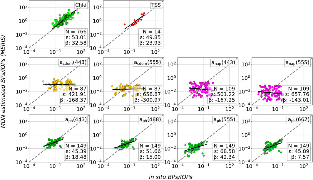
Figure 8. Scatter plots for comparison between MDN-estimated BPs/IOPs from MERIS satellite imagery and in situ measured BPs/IOPs from the SeaBASS dataset using co-located satellite-ground matchup samples. Satellite sampling times are matched with in situ sample collection times with a time interval within +/−3 h.

Figure 9 illustrates in situ BPs and IOPs plotted against their MDN counterparts from VIIRS data. The dataset includes 42 matchups for Chla, 23 matchups for a_ph, and very few matchups for TSS, a_cdom and a_nap (N < 10). Conversely, ε for variables such as Chla and TSS are moderate (71% and 79%). a_ph falls within the range of 19%–63%. Similar to the MERIS sensor, the retrieval of a_cdom and a_nap remains considerably poor. The slight error in a_ph (488) can be attributed to its high negative bias. Similarly, the bias for a_cdom and a_nap remains considerably high and adverse. The overall bias is high for TSS (79%), whereas a moderate bias is exhibited for Chla (28%). Other metrics discussed in Section 5 are shown in Supplementary Appendix Tables SB10-B13 for the SeaBASS dataset, corresponding to Figures 7–9. Due to the limited number of datasets used for this matchup analysis, it is challenging to thoroughly assess the performance of MDNs for the VIIRS sensor.

Figure 9

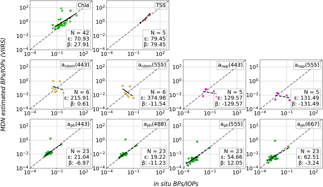
Figure 9. Scatter plots for comparison between MDN-estimated BPs/IOPs from VIIRS satellite imagery and in situ measured BPs/IOPs from the SeaBASS dataset using co-located satellite-ground matchup samples. Satellite sampling times are matched with in situ sample collection times with a time interval within +/−3 h.

5.2 Regional leave-one-out cross-validation

The validation results presented in the appendix (Supplementary Appendix Figures SA1-A3) demonstrate a reasonable estimation of BPs and IOPs when trained with 80% of the augmented GLORIA dataset. However, upon validation with SeaBASS and satellite matchups, it becomes apparent that the error nearly doubled compared to the performance achieved during training. This discrepancy raises concerns not only about the atmospheric correction procedure but also about the ability of a model to generalize to unseen test data. Given that the GLORIA dataset encompasses contributions from various researchers, laboratories, field campaigns, and water bodies, it is imperative to evaluate its individual sources to pinpoint potential issues.

To understand the impact of the data from each source within the development dataset, we conducted a series of LOO cross-validation experiments, akin to methodologies employed by previous studies (Pahlevan et al., 2022; O’Shea et al., 2023). Our approach involved iteratively training a MDN, excluding samples from specific sources or field campaigns in each iteration. The details of the individual datasets (Saranathan et al., 2024) are shown in Supplementary Appendix Table SB2. In these LOO experiments, the samples excluded from training in a particular trial are referred to as the left-out samples for that trial. Subsequently, we evaluated the models’ performance on samples from the excluded regions, which we term the “left-out test set.” For this evaluation, we computed and reported both predictive performances, utilizing ε mentioned in Section 4.1 as the primary indicator, and estimated uncertainty.

The LOO assessment of the MDN across three distinct sensors - MODIS, MERIS, and VIIRS - is visually presented in bar charts, illustrating results for all available data sources and each BP and IOP in Figure 10. Once again, the MDN demonstrates reasonable accuracy in estimating values across most datasets, indicating that, in general, the MDNs are able to generalize to previously unseen samples. That said the experiment also identifies specific dataset and parameter combinations where the model performance does not generalize as well as expected. Comparisons of MDN models with other standard models for BP and IOP retrievals are conducted in previous studies (Pahlevan et al., 2022; O’Shea et al., 2023), so we concentrate more on the consistency of ocean color sensors. It is important to note that individual regions with high ε do not suggest that the overall dataset is of low quality; rather, that the range of optical conditions and constituent concentrations from a specific dataset is not adequately represented within the broader dataset. The variance in performance among sensors can be attributed to the combination of bands available with each respective sensor.

Figure 10

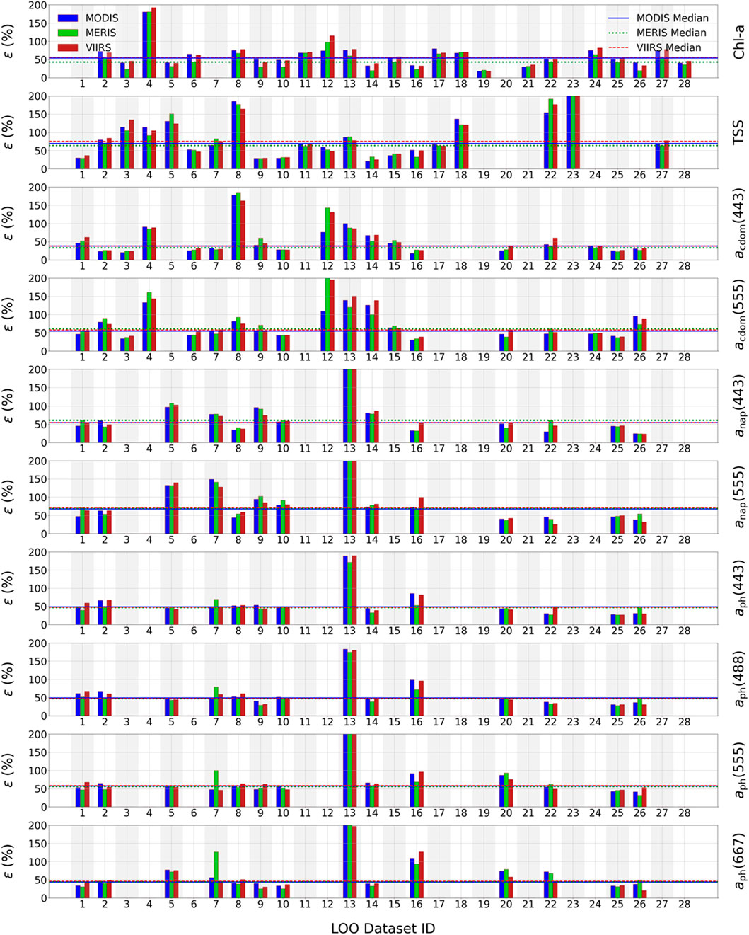
Figure 10. Performance assessments based on the LOO experiments utilizing the augmented GLORIA dataset for three different ocean color sensors (MODIS, MERIS and VIIRS) and 10 variables [Chla, TSS, a_cdom (440), a_cdom (555), a_nap (440), a_nap (555), a_ph (440), a_ph (488), a_ph (555), a_ph (667)]. See Supplementary Appendix Table SB2 for the details of the data sources and indices. The dotted lines represent the median of the MdSR from all 10 variables of BPs/IOPs.

The MDN consistently provides accurate estimates, with minor deviations observed for certain datasets. Notably, for Chla retrievals, dataset #4 exhibits slightly elevated error rates, whereas other datasets closely align with or slightly surpass the median ε value (horizontal line in Figure 10), demonstrating excellent accuracy. Similarly, in TSS retrieval, datasets #5, #8, #22, and #23 show notably higher error rates, while the remaining datasets exhibit performance close to or better than the median ε. For a_cdom retrieval, elevated errors are observed for datasets #8 and #12 at 443 nm, and datasets #4, #12, and #13 at 555 nm. Likewise, a_nap retrieval displays increased error rates for dataset #13 at 443 and 555 nm. However, the MDN demonstrates satisfactory performance for most datasets in these retrievals, except for dataset #13, which additionally exhibits elevated errors in a_ph retrieval.

It is crucial to note that these variations in error rates do not suggest inferior data quality. Rather, they can indicate that certain datasets have optical conditions or constituent concentrations that are not fully represented within the broader dataset. Comparing the three sensors, TSS retrievals exhibit the highest uncertainties, ranging from 64% for MERIS to 75% for VIIRS. The median ε values for each variable are calculated across the corresponding sensors (Supplementary Appendix Table S14). Notably, the reported uncertainties for all variables approximate to 54% across the three sensors. Considering all ten variables, VIIRS exhibits the highest ε values in comparison to the other two sensors, followed by MODIS and MERIS. Notably, BPs such as Chla and TSS consistently display an error rate of approximately 60% across all sensors in their retrievals. Moreover, the percentage error for all IOP retrievals remains relatively low, ranging from 33% to 71%. Similarly, IOP retrievals at all wavelengths exhibit comparatively lower errors (∼52%) when compared with BPs (∼60%).

These findings emphasize the subtle performance variations across sensors and highlight the importance of understanding the inherent characteristics of each of their bands in interpreting retrieval accuracies. Additionally, the consistency in error rates for specific variables and wavelengths offers valuable insights for refining retrieval algorithms and enhancing the overall accuracy of remote sensing data analysis. Understanding this slight difference in retrieval performance is vital for refining algorithms and enhancing the accuracy of remote sensing data interpretation. Further investigation into the underlying causes of discrepancies at specific stations can facilitate improvements in data processing techniques, ultimately advancing our ability to derive meaningful insights from remote sensing observations.

6 Spatial data analysis

In the previous section, we found a reasonable alignment between MODIS, MERIS, and VIIRS products and the MDN-based BPs and IOPs, particularly when compared to in situ datasets across coastal and inland waters. This section elucidates the efficacy of utilizing spatial data to comprehend the dynamic fluctuations in geophysical products within coastal and inland water bodies. Specifically, we focus on the Chesapeake Bay to analyze the MDN-based spatial products derived from MODIS, MERIS, and VIIRS. Situated along the East Coast of the United States, Chesapeake Bay encompasses highly productive waters, exhibiting a spectrum of phenomena including in-water blooms, suspended sediments, and dissolved materials across the bay and coastal regions.

Figure 11 presents MODIS/T (a) and MERIS (b) ocean color products showcasing the spatial distribution of BPs and IOPs on 27 December 2005, post-application of the MDN method. Leveraging the MDN retrievals, these images facilitate a clearer understanding of the spatial distribution of water quality parameters. Regions depicted in red indicate a high dominance of the corresponding water quality parameter, while those in blue signify a lower one. Figures 11a1, 11b1 illustrate the spatial variation of MDN-derived Chla as captured by MODIS/T and MERIS, respectively. The MODIS/T image vividly highlights the dominance of Chla near the shoreline in the northern and western parts of the bay. Conversely, the MERIS image exhibits less variation compared to MODIS, with less discernible features. The spatial variation of MDN-derived TSS, is depicted in Figures 11a2, 11b2 for MODIS/T and MERIS, respectively. In contrast to Chla, the dynamic changes in TSS distribution are readily discernible across the entire bay area and coastal waters in both MODIS/T and MERIS images.

Figure 11

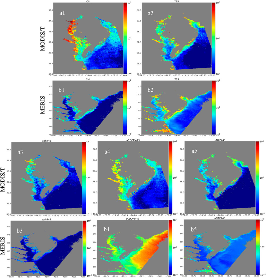
Figure 11. MODIS/T and MERIS based MDN-derived ocean color product images over the Chesapeake Bay, USA, acquired on December 27th, 2005. Panels (a1–a5) show MODIS/T products of BPs: (a1) Chla, (a2) TSS, and IOPs: (a3) a_ph, (a4) a_cdom, and (a5) a_nap at 443 nm. Panels (b1–b5) show MERIS products of BPs: (b1) Chla, (b2) TSS, and IOPs (b3) a_ph, (b4) a_cdom, and (b5) a_nap at 443 nm. All products were derived from SeaDAS corrected R_rs.

Similar to the BPs, the spatial distribution of the IOPs also distinctly reveals their variation in these optically complex waters. Figures 11a3, 11b3 highlight the presence of a_ph at 443 nm near the shoreline of the bay. The dominant features of the a_ph distribution are clearly depicted in the MODIS/T images, whereas they are less evident in the MERIS images. In Figures 11a4, 11b4, the distribution of a_cdom at 443 nm is distinctly visible, demonstrating that both MODIS/T and MERIS effectively capture the spatial distribution of dissolved organic matter over the bay area. This organic matter dissolves into the water due to tidal movements between the bay and the sea. The MODIS/T-acquired a_cdom image over the bay area aligns consistently with the MERIS-acquired a_cdom image. However, notable discrepancies arise offshore, where the two satellite images display significant variation. The spatial distribution of another crucial IOP variable, a_nap at 443 nm, is depicted in Figures 11a5, 11b5. Remarkably, the a_nap products obtained from both MODIS/T and MERIS sensors exhibit close consistency. Elevated levels of a_nap are observed predominantly along the shoreline of the bay and in coastal waters. This analysis distinctly elucidates that the BPs and IOPs derived from the MODIS/T and MERIS sensors exhibit consistency for TSS and a_nap, while slight variations are observed for other BPs and IOPs.

Figure 12 depicts MODIS/A (a) and VIIRS (b) ocean color products highlighting the spatial distribution of BPs and IOPs over Chesapeake Bay on 26 December 2018. Surprisingly, all ocean color products examined exhibit matching spatial distributions for both sensors. Evaluating the MDN-derived BPs Chla and TSS, as well as the IOPs, for consistency and spatial variability, clear patterns can be discerned. Figures 12a1, 12b1 illustrate the MDN-derived Chla levels detected by MODIS/A and VIIRS, respectively, denoting a notable concentration in the bay area and particularly along its shoreline. Conversely, Chla concentrations appear considerably lower in coastal and offshore waters. Noteworthy peaks in Chla are observed exclusively along the bay’s shoreline. The spatial distribution of MDN-derived TSS, is depicted in Figures 12a2, 12b2. Both MODIS/A and VIIRS ocean color products exhibit heightened TSS levels along the bay’s shoreline, with a consistent pattern, albeit slightly lower magnitudes in VIIRS compared to MODIS/A.

Figure 12

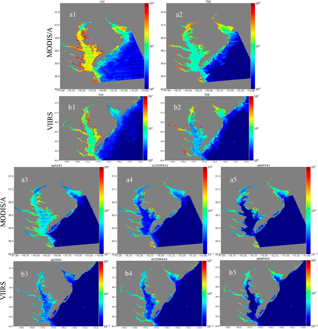
Figure 12. MODIS/A and VIIRS based MDN-derived ocean color product images over the Chesapeake Bay, USA, acquired on December 26th, 2018. Panels (a1–a5) show MODIS/A products of BPs: (a1) Chla, (a2) TSS, and IOPs: (a3) a_ph, (a4) a_cdom, and (a5) a_nap at 443 nm. Panels (b1–b5) show VIIRS products of BPs: (b1) Chla, (b2) TSS, and IOPs (b3) a_ph, (b4) a_cdom, and (b5) a_nap at 443 nm. All products were derived from SeaDAS corrected R_rs.

MDN-derived IOPs, such as a_ph, are coherent across both MODIS/A and VIIRS ocean color products, as demonstrated in Figures 12a3, 12b3. These images highlight an abundance of phytoplankton pigments within bay waters, especially in proximity to the shoreline, with minimal presence in offshore regions. This trend is replicated across both MODIS/A and VIIRS datasets. Similarly, Figures 12a4, 12b4 showcase the dominance of a_cdom in bay waters, with negligible quantities observed offshore. The spatial distribution of a_cdom, as estimated by the MDN, remains largely consistent across both platforms. Contrary to other IOPs, a_nap exhibits an uneven distribution within the bay zone, as depicted in Figures 12a5, 12b5. Non-algal particles are predominantly concentrated near the bay’s shoreline, coinciding with areas of heightened TSS levels (as shown in Figures 12a2, 12b2). Notably, the spatial patterns of MDN-derived a_nap remain highly similar for both MODIS/A and VIIRS imagery.

The consistency in spatial patterns between MODIS/A and VIIRS images suggests reliable performance in capturing ocean color variability over Chesapeake Bay. While minor differences exist in magnitude, overall trends remain consistent between the two sensors. Notably, both MODIS/A and VIIRS images show similar spatial distributions for MDN-derived BPs and IOPs. The comparative analysis indicates that MODIS/A and VIIRS sensors provide consistent and reliable ocean color products for monitoring the Chesapeake Bay, even though slight discrepancies exist, particularly with MERIS images.

7 Discussion

Recent studies have revealed the immense potential of satellite-based hyperspectral observations in enhancing our understanding of aquatic ecosystems on a global scale (O’Shea et al., 2023). However, the reliability of product retrievals tends to diminish with a multispectral sensor or equivalent reduction in the number of bands utilized. In our investigation, we scrutinized three different multispectral sensors - MODIS, MERIS, and VIIRS - each characterized by a distinct number of multispectral bands. Surprisingly, despite this variance, the accuracy of the MDN-estimated BPs and IOPs exhibited minimal discrepancy across the sensors, as depicted in the training results (first column, Figure 13), leveraging a substantial subset of 20% of the augmented GLORIA in situ dataset. Notably, we demonstrated that achieving a 20%–25% error margin in all BPs and IOPs utilizing MDNs is possible on in situ measured data. Slight disparities observed in the accuracy of BPs and IOP variables among the sensors can be attributed to differences in the available multispectral bands within each sensor.

Figure 13

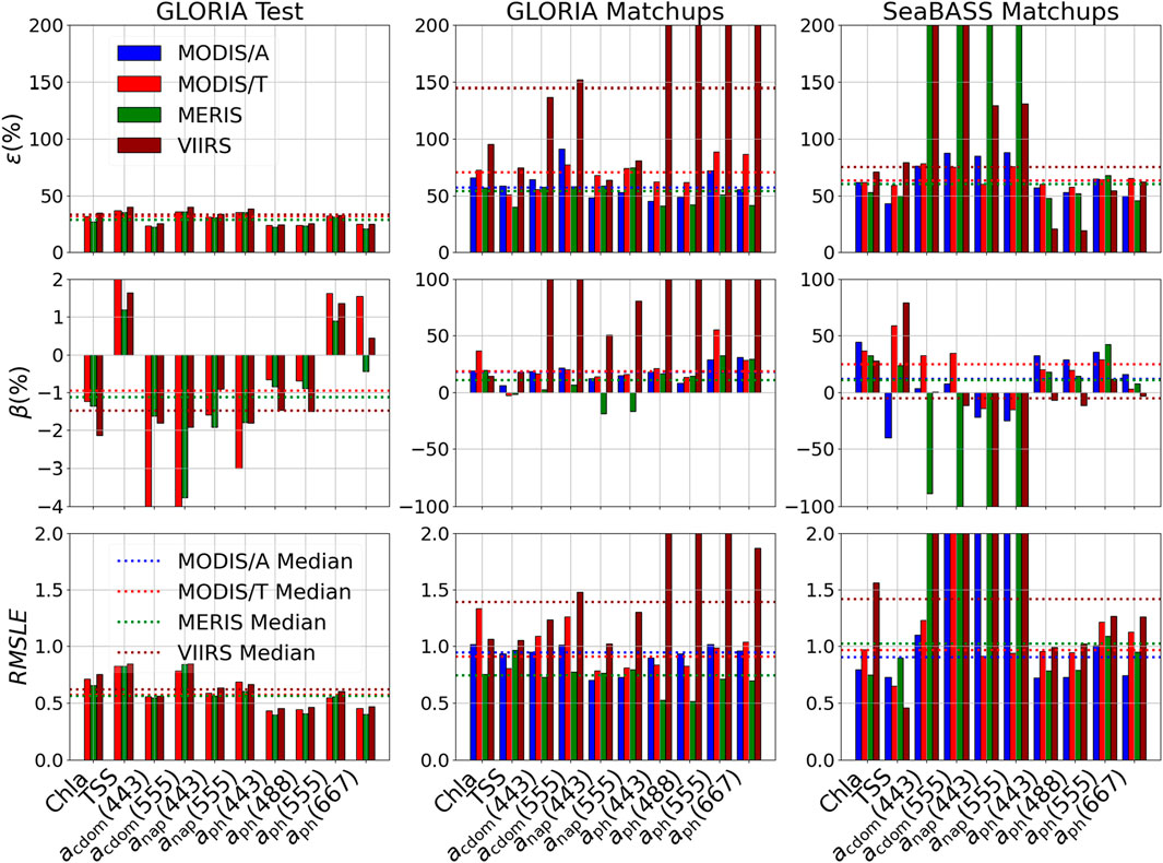
Figure 13. Bar chart representation of MdSR derived from three distinct MDN estimates: GLORIA Test dataset, GLORIA matchups and SeaBASS matchups across three different sensors. The dotted lines represent the median of the MdSR from all 10 variables of BPs/IOPs.

The heritage AC model represents a significant advancement in the field, delivering improved $R_{rs}$ products compared to prior studies (Pahlevan et al., 2024). However, challenges persist, particularly in highly productive aquatic environments where negative retrievals are frequently encountered. These discrepancies introduce uncertainties, especially in extrapolating aerosol contributions to the blue region of the $R_{rs}$ spectrum (Frouin et al., 2019). Such uncertainties reverberate throughout downstream products like BPs and IOPs, as evidenced in this study. For example, our analysis reveals that residual errors in $R_{rs}$ lead to approximately 50% overestimation across key parameters such as Chla, TSS, a_cdom, a_nap, and a_ph (second column, Figure 13) for the same GLORIA dataset. Here, satellite $R_{rs}$ is used as the input for the MDN model. The geographical distribution of GLORIA matchups (+/−3 h) with their year wise distribution for these ocean color missions are shown in the appendix (Supplementary Appendix Figures SA6, A7). The scatterplots and performance metrics for GLORIA matchups with MODIS, MERIS, and VIIRS are presented in the appendix as well (Supplementary Appendix Figures SA8, A11 and Supplementary Appendix Tables SB6-B9) and illustrate how issues in atmospheric correction directly impact $R_{rs}$ and consequently influence the water quality variables.

The results highlight that MODIS use of both NIR and SWIR bands enables effective atmospheric correction, minimizing atmospheric effects. While VIIRS employs a similar approach, its limited visible bands restrict its ability to resolve complex optical properties in aquatic environments, affecting the retrieval of inherent optical properties (IOPs) like a_cdom and a_nap. MERIS, with a broader visible spectrum, offers better spectral resolution, but relies solely on NIR bands for atmospheric correction, potentially introducing biases under certain conditions. These limitations in VIIRS and MERIS atmospheric correction and band configurations may lead to lower a_cdom and a_nap estimates. The validation dataset for VIIRS, particularly for a_cdom and a_nap, is limited, potentially affecting the robustness of these specific validations. To address this, the Appendix includes MDN performance evaluations for the GLORIA dataset and VIIRS sensor, offering initial insights into model capabilities. While matchups for a_cdom and a_nap are sparse, the datasets cover diverse global waters, supporting the MDN’s applicability across multiple variables. Additionally, we highlight the model’s performance on other water quality indicators, such as Chla, TSS, and a_ph, where data coverage is more comprehensive, providing a broader and more reliable evaluation of its capabilities.

The third column (Figure 13) shows the performance metrics for the SeaBASS matchups with the three satellite sensors. As we discussed in Section 5.1, the error still increased approximately 75%. It is plausible that these inaccuracies stem not only from the model and atmospheric correction, but also from factors such as inadequate vicarious calibrations, residual biases in TOA measurements (Ibrahim et al., 2018), and adjacency effects (Sterckx et al., 2011). Our findings strongly suggest that the MDN is particularly susceptible to errors in atmospheric correction (Zolfaghari et al., 2023) and adjacency effects. Addressing these challenges requires a concerted effort of both refining the models and emphasizing the critical need for accurate atmospheric correction in aquatic remote sensing studies.

8 Conclusion

This study introduces an MDN-based inversion method tailored for the concurrent estimation of Chla, TSS, a_cdom, a_nap, and a_ph from $R_{rs}$ across a range of multispectral ocean color sensors, applicable to coastal and inland water bodies. By training the MDN model using additional IOP data aligned with 80% of the augmented GLORIA dataset, better accuracy is achieved. Notably, the model demonstrates enhanced or comparable accuracy (ranging from 15% to 40% across all products) when validated against a larger and more diverse in situ dataset compared to prior dedicated MDN approaches. Validation of the SeaBASS dataset against MODIS, MERIS, and VIIRS satellite datasets through matchup analysis further underscores the robustness of the model, with accuracy ranging from 40% to 70% across all BPs and IOPs.

Leveraging a regional leave-one-out cross-validation approach, the MDN exhibits superior generalization performance across various sensor platforms and water types. Furthermore, this study elucidates the suitability of MDN models for specific regional water bodies and identifies sensors that offer better accuracy for individual BPs and IOPs. The results of the leave-one-out analysis reveal minimal discrepancies among the retrievals from the three ocean color sensors. When applied to satellite images, slight differences between MODIS, MERIS, and VIIRS are observed, primarily attributed to atmospheric correction algorithm nuances and sensor band disparities.

Addressing the substantial uncertainty stemming from atmospheric correction underscores the potential for significant accuracy enhancements in IOP retrieval through improved remote sensing reflectance retrieval techniques. Future refinements to the MDN approach could incorporate additional environmental and physical variables as input features, facilitating phytoplankton type/species discrimination within specific geographic regions. In this study, the MDN approach was applied exclusively to heritage ocean color sensors, driven by the absence of a matchup validation dataset for recent ocean sensors. The availability of in situ data presents an opportunity to expand this methodology to recent multispectral sensors such as VIIRS onboard NOAA-20 and NOAA-21 and OLCI onboard Sentinel-3A and Sentinel-3B. These advancements hold promise for enhancing monitoring capabilities of water bodies.

Data availability statement

The raw data supporting the conclusions of this article will be made available by the authors, without undue reservation.

Author contributions

SB: Writing–original draft, Writing–review and editing, Conceptualization, Data curation, Investigation, Methodology, Software, Validation, Visualization. RO’S: Formal Analysis, Methodology, Software, Writing–original draft, Writing–review and editing. AS: Formal Analysis, Methodology, Software, Writing–original draft, Writing–review and editing. ChB: Data curation, Methodology, Software, Writing–review and editing. DG: Data curation, Writing–original draft, Writing–review and editing. CaB: Writing–review and editing. CG: Writing–review and editing. MT: Writing–review and editing. KA: Writing–review and editing. KK: Writing–review and editing. ML: Writing–review and editing. LR: Writing–review and editing.

Funding

The author(s) declare that financial support was received for the research, authorship, and/or publication of this article. This work was supported in part by the National Aeronautics and Space Administration (NASA) Research Opportunities in Space and Earth Sensing (ROSES) under grant 80NSSC22K1389 (RSWQ21) associated with Remote Sensing of Water Quality.

Acknowledgments

The authors would also like to express our deep appreciation to the Project Investigators and supporting staff involved in the data collection process for their invaluable contributions to the GLORIA and the SeaBASS databases. We specifically acknowledge the efforts of these data contributors and their teams, including: Ms. Janet Anstee (Commonwealth Scientific and Industrial Research Organisation (CSIRO), Australia), Dr. Cláudio C. F. Barbosa (Instrumentation Lab for Aquatic Systems (LabISA), National Institute for Space Research (INPE), Brazil), Dr. Patrick L. Brezonik (Department of Civil, Environmental, and Geo-Engineering, University of Minnesota, United States), Dr. Zhingang Cao (Nanjing Institute of Geography and Limnology, Chinese Academy of Sciences, China), Dr. Arnold G. Dekker (SatDek Pty Ltd, Australia), Dr. Dariusz Ficek (Institute of Biology and Earth Sciences, Pomeranian University, Poland), Dr. Dalin Jiang (Earth and Planetary Observation Sciences (EPOS), Biological and Environmental Sciences, Faculty of Natural Sciences, University of Stirling, United Kingdom), Dr. Arne S. Kristoffersen (Department of Physics and Technology, University of Bergen, Norway), Dr. David M. O’Donnell (Upstate Freshwater Institute, United States), Dr. Leif G. Olmanson (Department of Forest Resources, University of Minnesota, United States), Dr. Antonio Ruiz Verdú (Laboratory for Earth Observation, University of Valencia, Spain), Dr. Stefan G.H. Simis (Plymouth Marine Laboratory, Plymouth, United Kingdom), Dr. Ian Somlai-Schweiger (German Aerospace Center (DLR), Remote Sensing Technology Institute, Germany), Dr. Hans J. van der Woerd (Department of Water and Climate Risk, Institute for Environmental Studies (IVM), Netherlands), and Dr. Courtney Di Vittorio (Wake Forest University, Engineering, United States), for their invaluable contributions in preparing the augmented dataset of the GLORIA that includes enhanced water quality parameters. Your dedication and expertise have been instrumental in advancing this work. Finally, we express our heartfelt gratitude to Dr. Nima Pahlevan, Program Manager at NASA Headquarters, for his exceptional collaboration and unwavering support throughout this work.

Conflict of interest

Author SB was employed by Geosensing and Imaging Consultancy. Authors RO’S, AS, and ChB were employed by Science Systems and Applications Inc. Author ChB was employed by BAE Systems. Author ML was employed by Starboard Maritime Intelligence.

The remaining authors declare that the research was conducted in the absence of any commercial or financial relationships that could be construed as a potential conflict of interest.

Publisher’s note

All claims expressed in this article are solely those of the authors and do not necessarily represent those of their affiliated organizations, or those of the publisher, the editors and the reviewers. Any product that may be evaluated in this article, or claim that may be made by its manufacturer, is not guaranteed or endorsed by the publisher.

Supplementary material

The Supplementary Material for this article can be found online at: https://www.frontiersin.org/articles/10.3389/frsen.2025.1488565/full#supplementary-material

References

Babin, M., Stramski, D., Ferrari, G. M., Claustre, H., Bricaud, A., Obolensky, G., et al. (2003). Variations in the light absorption coefficients of phytoplankton, nonalgal particles, and dissolved organic matter in coastal waters around Europe. J. Geophys. Res. Ocean. 108. doi:10.1029/2001jc000882

CrossRef Full Text | Google Scholar

Bailey, S. W., Franz, B. A., Jeremy Werdell, P., Gordon, H. R., Wang, M., Siegel, D. A., et al. (2010). Estimation of near-infrared water-leaving reflectance for satellite ocean color data processing. Opt. Express 18, 7521–7527. doi:10.1364/oe.18.007521

PubMed Abstract | CrossRef Full Text | Google Scholar

Balasubramanian, S. V., Pahlevan, N., Smith, B., Binding, C., Schalles, J., Loisel, H., et al. (2020). Robust algorithm for estimating total suspended solids (TSS) in inland and nearshore coastal waters. Remote Sens. Environ. 246, 111768. doi:10.1016/j.rse.2020.111768

CrossRef Full Text | Google Scholar

Barnes, B. B., Cannizzaro, J. P., English, D. C., and Hu, C. (2019). Validation of VIIRS and MODIS reflectance data in coastal and oceanic waters: an assessment of methods. Remote Sens. Environ. 220, 110–123. doi:10.1016/j.rse.2018.10.034

CrossRef Full Text | Google Scholar

Bartram, J., and Ballance, R. (1996). Water Quality Monitoring: a practical guide to the design and implementation of freshwater quality studies and monitoring programmes. 1st ed. CRC Press. doi:10.1201/9781003062110

CrossRef Full Text | Google Scholar

Behrenfeld, M. J., O’Malley, R. T., Siegel, D. A., McClain, C. R., Sarmiento, J. L., Feldman, G. C., et al. (2006). Climate-driven trends in contemporary ocean productivity. Nature 444, 752–755. doi:10.1038/nature05317

PubMed Abstract | CrossRef Full Text | Google Scholar

Binding, C. E., Jerome, J. H., Bukata, R. P., and Booty, W. G. (2008). Spectral absorption properties of dissolved and particulate matter in Lake Erie. Remote Sens. Environ. 112, 1702–1711. doi:10.1016/j.rse.2007.08.017

CrossRef Full Text | Google Scholar

Binding, C. E., Pizzolato, L., and Zeng, C. (2021). EOLakeWatch; delivering a comprehensive suite of remote sensing algal bloom indices for enhanced monitoring of Canadian eutrophic lakes. Ecol. Indic. 121, 106999. doi:10.1016/j.ecolind.2020.106999

CrossRef Full Text | Google Scholar

Bishop, C. M. (1994). Mixture density networks. Birmingham, U.K: Aston University.

Google Scholar

Bishop, C. M. (1995). Neural networks for pattern recognition. Oxford University Press.

Google Scholar

Bowers, D. G., and Binding, C. E. (2006). The optical properties of mineral suspended particles: a review and synthesis. Estuar. Coast. Shelf Sci. 67, 219–230. doi:10.1016/j.ecss.2005.11.010

CrossRef Full Text | Google Scholar

Brewin, R. J. W., Pitarch, J., Dall’Olmo, G., van der Woerd, H. J., Lin, J., Sun, X., et al. (2023). Evaluating historic and modern optical techniques for monitoring phytoplankton biomass in the Atlantic Ocean. Front. Mar. Sci. 10, 1111416. doi:10.3389/fmars.2023.1111416

CrossRef Full Text | Google Scholar

Brezonik, P. L., Olmanson, L. G., Finlay, J. C., and Bauer, M. E. (2015). Factors affecting the measurement of CDOM by remote sensing of optically complex inland waters. Remote Sens. Environ. 157, 199–215. doi:10.1016/j.rse.2014.04.033

CrossRef Full Text | Google Scholar

Bricaud, A., Babin, M., Morel, A., and Claustre, H. (1995). Variability in the chlorophyll-specific absorption coefficients of natural phytoplankton: analysis and parameterization. J. Geophys. Res. 100, 13321–13332. doi:10.1029/95jc00463

CrossRef Full Text | Google Scholar

Bricaud, A., Claustre, H., Ras, J., and Oubelkheir, K. (2004). Natural variability of phytoplanktonic absorption in oceanic waters: influence of the size structure of algal populations. J. Geophys. Res. Ocean. 109, 1–12. doi:10.1029/2004jc002419

CrossRef Full Text | Google Scholar

Bricaud, A., Mejia, C., Blondeau-Patissier, D., Claustre, H., Crepon, M., and Thiria, S. (2007). Retrieval of pigment concentrations and size structure of algal populations from their absorption spectra using multilayered perceptrons. Appl. Opt. 46, 1251. doi:10.1364/AO.46.001251

PubMed Abstract | CrossRef Full Text | Google Scholar

Bricaud, A., Morel, A., Babin, M., Allali, K., and Claustre, H. (1998). Variations of light absorption by suspended particles with chlorophyll a concentration in oceanic (case 1) waters: analysis and implications for bio-optical models. J. Geophys. Res. Ocean. 103, 31033–31044. doi:10.1029/98jc02712

CrossRef Full Text | Google Scholar

Bricaud, A., Morel, A., and Prieur, L. (1981). Absorption by dissolved organic matter of the sea (yellow substance) in the UV and visible domains. Limnol. Oceanogr. 26, 43–53. doi:10.4319/lo.1981.26.1.0043

CrossRef Full Text | Google Scholar

Brown, C. M., Lund, J. R., Cai, X., Reed, P. M., Zagona, E. A., Ostfeld, A., et al. (2015). The future of water resources systems analysis: toward a scientific framework for sustainable water management. Water Resour. Res. 51, 6110–6124. doi:10.1002/2015wr017114

CrossRef Full Text | Google Scholar

Burket, M. O., Olmanson, L. G., and Brezonik, P. L. (2023). Comparison of two water color algorithms: implications for the remote sensing of water bodies with moderate to high CDOM or chlorophyll levels. Sensors 23, 1071. doi:10.3390/s23031071

PubMed Abstract | CrossRef Full Text | Google Scholar

Buuren, S. V., and Groothuis-Oudshoorn, K. (2010). MICE: multivariate imputation by chained equations in R. J. Stat. Softw. 1–68. doi:10.18637/jss.v045.i03

CrossRef Full Text | Google Scholar

Cannizzaro, J. P., Barnes, B. B., Hu, C., Corcoran, A. A., Hubbard, K. A., Muhlbach, E., et al. (2019). Remote detection of cyanobacteria blooms in an optically shallow subtropical lagoonal estuary using MODIS data. Remote Sens. Environ. 231, 111227. doi:10.1016/j.rse.2019.111227

CrossRef Full Text | Google Scholar

Cao, Z., Duan, H., Shen, M., Ma, R., Xue, K., Liu, D., et al. (2018). Using VIIRS/NPP and MODIS/Aqua data to provide a continuous record of suspended particulate matter in a highly turbid inland lake. Int. J. Appl. Earth Obs. Geoinf. 64, 256–265. doi:10.1016/j.jag.2017.09.012

CrossRef Full Text | Google Scholar

Cao, Z., Hu, C., Ma, R., Duan, H., Liu, M., Loiselle, S., et al. (2023). MODIS observations reveal decrease in lake suspended particulate matter across China over the past two decades. Remote Sens. Environ. 295, 113724. doi:10.1016/j.rse.2023.113724

CrossRef Full Text | Google Scholar

Cao, Z., Ma, R., Pahlevan, N., Liu, M., Melack, J. M., Duan, H., et al. (2022). Evaluating and optimizing VIIRS retrievals of chlorophyll-a and suspended particulate matter in turbid lakes using a machine learning approach. IEEE Trans. Geosci. Remote Sens. 60, 1–17. doi:10.1109/tgrs.2022.3220529

CrossRef Full Text | Google Scholar

Carder, K. (1997). “Okeechobee. SeaWiFS bio-optical archive and storage System (SeaBASS),”. NASA. doi:10.5067/SeaBASS/OKEECHOBEE/DATA001

CrossRef Full Text | Google Scholar

Carder, K. (1998). TOTO. SeaWiFS bio-optical archive and storage System (SeaBASS), NASA. doi:10.5067/SeaBASS/TOTO/DATA001

CrossRef Full Text | Google Scholar

Carder, K., and Hu, C. (2005). “West_Florida_Shelf,”. SeaWiFS Bio-optical Archive Storage Syst. (SeaBASS). doi:10.5067/SeaBASS/WEST_FLORIDA_SHELF/DATA001

CrossRef Full Text | Google Scholar

Carder, K., and Kirkpatrick, G. (1998). RED_TIDE. SeaWiFS bio-optical archive and storage System (SeaBASS). doi:10.5067/SeaBASS/RED_TIDE/DATA001

CrossRef Full Text | Google Scholar

Carder, K., and Mitchell, G. (1999). “ECOHAB. SeaWiFS bio-optical archive and storage System (SeaBASS),”. NASA. doi:10.5067/SeaBASS/ECOHAB/DATA001

CrossRef Full Text | Google Scholar

Casey, K. A., Rousseaux, C. S., Gregg, W. W., Boss, E., Chase, A. P., Craig, S. E., et al. (2020). A global compilation of in situ aquatic high spectral resolution inherent and apparent optical property data for remote sensing applications. Earth Syst. Sci. Data 12, 1123–1139. doi:10.5194/essd-12-1123-2020

PubMed Abstract | CrossRef Full Text | Google Scholar

Clark, D. K., Gordon, H. R., Voss, K. J., Ge, Y., Broenkow, W., and Treess, C. (1997). Validation of atmospheric correction over the oceans. J. Geophys. Res. Atmos. 102, 17209–17217. doi:10.1029/96jd03345

CrossRef Full Text | Google Scholar

Cota, G., and Zimmerman, R. (2000). “Chesapeake_Light_Tower,” in SeaWiFS bio-optical archive and storage System (SeaBASS). NASA. doi:10.5067/SeaBASS/CHESAPEAKE_LIGHT_TOWER/DATA001

CrossRef Full Text | Google Scholar

Cui, T., Zhang, J., Groom, S., Sun, L., Smyth, T., and Sathyendranath, S. (2010). Validation of MERIS ocean-color products in the Bohai Sea: a case study for turbid coastal waters. Remote Sens. Environ. 114, 2326–2336. doi:10.1016/j.rse.2010.05.009

CrossRef Full Text | Google Scholar

Cui, T., Zhang, J., Tang, J., Sathyendranath, S., Groom, S., Ma, Y., et al. (2014). Assessment of satellite ocean color products of MERIS, MODIS and SeaWiFS along the East China coast (in the yellow sea and East China sea). ISPRS J. Photogramm. Remote Sens. 87, 137–151. doi:10.1016/j.isprsjprs.2013.10.013

CrossRef Full Text | Google Scholar

Delgado, A. L., Guinder, V. A., Dogliotti, A. I., Zapperi, G., and Pratolongo, P. D. (2019). Validation of MODIS-Aqua bio-optical algorithms for phytoplankton absorption coefficient measurement in optically complex waters of El Rincón (Argentina). Cont. Shelf Res. 173, 73–86. doi:10.1016/j.csr.2018.12.012

CrossRef Full Text | Google Scholar

Devred, E., Perry, T., and Massicotte, P. (2022). Seasonal and decadal variations in absorption properties of phytoplankton and non-algal particulate matter in three oceanic regimes of the Northwest Atlantic. Front. Mar. Sci. 9, 1–19. doi:10.3389/fmars.2022.932184

CrossRef Full Text | Google Scholar

Fan, Y., Li, W., Chen, N., Ahn, J. H., Park, Y. J., Kratzer, S., et al. (2021). OC-SMART: a machine learning based data analysis platform for satellite ocean color sensors. Remote Sens. Environ. 253, 112236. doi:10.1016/j.rse.2020.112236

CrossRef Full Text | Google Scholar

Fickas, K. C., O’Shea, R. E., Pahlevan, N., Smith, B. B. S., and Wolny, J. L. (2023). Leveraging multimission satellite data for spatiotemporally coherent cyanoHAB monitoring. Front. Remote Sens. 4, 1157609. doi:10.3389/frsen.2023.1157609

CrossRef Full Text | Google Scholar

Frouin, R. J., Franz, B. A., Ibrahim, A., Knobelspiesse, K., Ahmad, Z., Cairns, B., et al. (2019). Atmospheric correction of satellite ocean-color imagery during the PACE era. Front. Earth Sci. 7, 1–43. doi:10.3389/feart.2019.00145

PubMed Abstract | CrossRef Full Text | Google Scholar

Galimard, J. E., Chevret, S., Curis, E., and Resche-Rigon, M. (2018). Heckman imputation models for binary or continuous MNAR outcomes and MAR predictors. BMC Med. Res. Methodol. 18, 90. doi:10.1186/s12874-018-0547-1

PubMed Abstract | CrossRef Full Text | Google Scholar

Garaba, S. P., Wernand, M. R., and Zielinski, O. (2011). Quality control of automated hyperspectral remote sensing measurements from a seaborne platform. Ocean. Sci. Discuss. 8, 613–638. doi:10.5194/osd-8-613-2011

CrossRef Full Text | Google Scholar

Garcia, R. A., Lee, Z., Barnes, B. B., Hu, C., Dierssen, H. M., and Hochberg, E. J. (2020). Benthic classification and iop retrievals in shallow water environments using meris imagery. Remote Sens. Environ. 249, 112015. doi:10.1016/j.rse.2020.112015

CrossRef Full Text | Google Scholar

Ghahramani, Z., and Jordan, M. I. (1995). Learning from incomplete data.

Google Scholar

Gonçalves-Araujo, R., Rabe, B., Peeken, I., and Bracher, A. (2018). High colored dissolved organic matter (CDOM) absorption in surface waters of the central-eastern Arctic Ocean: implications for biogeochemistry and ocean color algorithms. PLoS ONE 13 (1), e0190838. doi:10.1371/journal.pone.0190838

PubMed Abstract | CrossRef Full Text | Google Scholar

Gordon, H. R., Brown, O. B., Evans, R. H., Brown, J. W., Smith, R. C., Baker, K. S., et al. (1988). A semianalytic radiance model of ocean color. J. Geophys. Res. 93, 10909–10924. doi:10.1029/jd093id09p10909

CrossRef Full Text | Google Scholar

Gordon, H. R., Brown, O. B., and Jacobs, M. M. (1975). Computed relationships between the inherent and apparent optical properties of a flat homogeneous ocean. Appl. Opt. 14, 417. doi:10.1364/ao.14.000417

PubMed Abstract | CrossRef Full Text | Google Scholar

Gordon, H. R., and Wang, M. (1994). Retrieval of water-leaving radiance and aerosol optical thickness over the oceans with SeaWiFS: a preliminary algorithm. Appl. Opt. 33, 443. doi:10.1364/ao.33.000443

PubMed Abstract | CrossRef Full Text | Google Scholar

Hill, V., and Zimmerman, R. (2010). “Seagrass_Mapping_Florida,” in SeaWiFS bio-optical archive and storage System (SeaBASS). NASA. doi:10.5067/SeaBASS/SEAGRASS_MAPPING_FLORIDA/DATA001

CrossRef Full Text | Google Scholar

Hoge, F. E., and Lyon, P. E. (1996). Satellite retrieval of inherent optical properties by linear matrix inversion of oceanic radiance models: an analysis of model and radiance measurement errors. J. Geophys. Res. 101, 16631–16648. doi:10.1029/96jc01414

CrossRef Full Text | Google Scholar

Hooker, S. B., and McClain, C. R. (2000). The calibration and validation of SeaWiFS data. Prog. Oceanogr. 45, 427–465. doi:10.1016/s0079-6611(00)00012-4

CrossRef Full Text | Google Scholar

Hu, C., and Le, C. (2014). Ocean color continuity from VIIRS measurements over tampa bay. IEEE Geosci. Remote Sens. Lett. 11, 945–949. doi:10.1109/lgrs.2013.2282599

CrossRef Full Text | Google Scholar

Hu, C., Li, D., Chen, C., Ge, J., Muller-Karger, F. E., Liu, J., et al. (2010). On the recurrent ulva prolifera blooms in the yellow sea and East China sea. J. Geophys. Res. Ocean. 115, 1–8. doi:10.1029/2009jc005561

CrossRef Full Text | Google Scholar

Hu, C., and Muller-Karger, F. (2012). “SFP. SeaWiFS bio-optical archive and storage System (SeaBASS),”. NASA. doi:10.5067/SeaBASS/SFP/

CrossRef Full Text | Google Scholar

Huan, Y., Sun, D., Wang, S., Zhang, H., Qiu, Z., Bilal, M., et al. (2021). Remote sensing estimation of phytoplankton absorption associated with size classes in coastal waters. Ecol. Indic. 121, 107198. doi:10.1016/j.ecolind.2020.107198

CrossRef Full Text | Google Scholar

Ibrahim, A., Franz, B., Ahmad, Z., Healy, R., Knobelspiesse, K., Gao, B. C., et al. (2018). Atmospheric correction for hyperspectral ocean color retrieval with application to the hyperspectral imager for the Coastal Ocean (HICO). Remote Sens. Environ. 204, 60–75. doi:10.1016/j.rse.2017.10.041

CrossRef Full Text | Google Scholar

IOCCG (2008). “Why Ocean colour? The societal benefits of ocean-colour Technology,” in Reports of the international ocean-colour coordinating group, No. 7. Editors T. Platt, N. Hoepffner, V. Stuart, and C. Brown (Dartmouth, Canada: IOCCG).

Google Scholar

IOCCG (2009). “Partition of the ocean into ecological provinces: role of ocean-colour radiometry,” in Reports of the international ocean-colour coordinating group, No. 9. Editors M. Dowell, and T. Platt (Dartmouth, Canada: IOCCG).

Google Scholar

IOCCG (2014). “Phytoplankton functional types from space,” in Reports of the international ocean-colour coordinating group, No. 15. Editor S. Sathyendranath (Dartmouth, Canada: IOCCG), 2014.

Google Scholar

Jamet, C., Loisel, H., and Dessailly, D. (2012). Retrieval of the spectral diffuse attenuation coefficientK_d(λ) in open and coastal ocean waters using a neural network inversion. J. Geophys. Res. Oceans 117. doi:10.1029/2012jc008076

CrossRef Full Text | Google Scholar

Jane, S. F., Hansen, G. J. A., Kraemer, B. M., Leavitt, P. R., Mincer, J. L., North, R. L., et al. (2021). Widespread deoxygenation of temperate lakes. Nature 594, 66–70. doi:10.1038/s41586-021-03550-y

PubMed Abstract | CrossRef Full Text | Google Scholar

Jiang, D., Matsushita, B., Pahlevan, N., Gurlin, D., Lehmann, M. K., Fichot, C. G., et al. (2021). Remotely estimating total suspended solids concentration in clear to extremely turbid waters using a novel semi-analytical method. Remote Sens. Environ. 258, 112386. doi:10.1016/j.rse.2021.112386

CrossRef Full Text | Google Scholar

Kallio, K., Kutser, T., Hannonen, T., Koponen, S., Pulliainen, J., Veps ̈ala ̈inen, J., et al. (2001). Retrieval of water quality from airborne imaging spectrometry of various lake types in different seasons. Sci. Total Environ. 268, 59–77. doi:10.1016/s0048-9697(00)00685-9

PubMed Abstract | CrossRef Full Text | Google Scholar

Knaeps, E., Doxaran, D., Dogliotti, A., Nechad, B., Ruddick, K., Raymaekers, D., et al. (2018). The SeaSWIR dataset. Sci. Data 10, 1439–1449. doi:10.5194/essd-10-1439-2018

CrossRef Full Text | Google Scholar

Lai, L., Liu, Y., Zhang, Y., Cao, Z., Yang, Q., and Chen, X. (2023). MODIS Terra and Aqua images bring non-negligible effects to phytoplankton blooms derived from satellites in eutrophic lakes. Water Res. 246, 120685. doi:10.1016/j.watres.2023.120685

PubMed Abstract | CrossRef Full Text | Google Scholar

Lavigne, H., Dogliotti, A., Doxaran, D., Shen, F., Castagna, A., Beck, M., et al. (2022). The HYPERMAQ dataset: bio-optical properties of moderately to extremely turbid waters. Earth Syst. Sci. Data 14, 4935–4947. doi:10.5194/essd-14-4935-2022

CrossRef Full Text | Google Scholar

Lee, Z., Carder, K. L., and Arnone, R. A. (2002). Deriving inherent optical properties from water color: a multiband quasi-analytical algorithm for optically deep waters. Appl. Opt. 41, 5755. doi:10.1364/ao.41.005755

PubMed Abstract | CrossRef Full Text | Google Scholar

Lehmann, M. K., Gurlin, D., Pahlevan, N., Alikas, K., Anstee, J., Balasubramanian, S. V., et al. (2023). GLORIA - a globally representative hyperspectral in situ dataset for optical sensing of water quality. Sci. Data 10, 100. doi:10.1038/s41597-023-01973-y

PubMed Abstract | CrossRef Full Text | Google Scholar

Lima, T. M. A. d., Giardino, C., Bresciani, M., Barbosa, C. C. F., Fabbretto, A., Pellegrino, A., et al. (2023). Assessment of estimated phycocyanin and chlorophyll-a concentration from PRISMA and OLCI in Brazilian inland waters: a comparison between semi-analytical and machine learning algorithms. Remote Sens. 15, 1299. doi:10.3390/rs15051299

CrossRef Full Text | Google Scholar

Liu, X., Warren, M., Selmes, N., and Simis, S. G. (2024). Quantifying decadal stability of lake reflectance and chlorophyll-a from medium-resolution ocean color sensors. Remote Sens. Environ. 306, 114120. doi:10.1016/j.rse.2024.114120

CrossRef Full Text | Google Scholar

Maciel, D. A., Barbosa, C. C. F., Martins, V. S., Smith, B., O'Shea, R. E., Balasubramanian, S. V., et al. (2023). Towards global long-term water transparency products from the Landsat archive. Remote Sens. Environ. 299, 113889. doi:10.1016/j.rse.2023.113889

CrossRef Full Text | Google Scholar

Mannino, A., Novak, M. G., Hooker, S. B., Hyde, K., and Aurin, D. (2014). Algorithm development and validation of CDOM properties for estuarine and continental shelf waters along the northeastern U.S. coast. Remote Sens. Environ. 152, 576–602. doi:10.1016/j.rse.2014.06.027

CrossRef Full Text | Google Scholar

Maritorena, S., Siegel, D. A., and Peterson, A. R. (2002). Optimization of a semianalytical ocean color model for global-scale applications. Appl. Opt. 41, 2705. doi:10.1364/ao.41.002705

PubMed Abstract | CrossRef Full Text | Google Scholar

Marra, J., Nelson, N., Siegel, D., and Vaillancourt, R. (1988). “BBOP. SeaWiFS bio-optical archive and storage System (SeaBASS),”. NASA. doi:10.5067/SeaBASS/BBOP/DATA001

CrossRef Full Text | Google Scholar

McClain, C. R. (2009). A decade of satellite ocean color observations. Ann. Rev. Mar. Sci. 1, 19–42. doi:10.1146/annurev.marine.010908.163650

PubMed Abstract | CrossRef Full Text | Google Scholar

McKinna, L. I. W., Fearns, P. R. C., Weeks, S. J., Werdell, P. J., Reichstetter, M., Franz, B. A., et al. (2015). A semianalytical ocean color inversion algorithm with explicit water column depth and substrate reflectance parameterization. J. Geophys. Res. Oceans 120, 1741–1770. doi:10.1002/2014JC010224

CrossRef Full Text | Google Scholar

Mélin, F., Zibordi, G., and Berthon, J. F. (2007). Assessment of satellite ocean color products at a coastal site. Remote Sens. Environ. 110, 192–215. doi:10.1016/j.rse.2007.02.026

CrossRef Full Text | Google Scholar

Mobley, C. D. (1999). Estimation of the remote-sensing reflectance from above-surface measurements. Appl. Opt. 38, 7442. doi:10.1364/ao.38.007442

PubMed Abstract | CrossRef Full Text | Google Scholar

Montes-Hugo, M., and Xie, H. (2015). An inversion model based on salinity and remote sensing reflectance for estimating the phytoplankton absorption coefficient in the Saint Lawrence Estuary. J. Geophys. Res. Oceans 120, 6958–6970. doi:10.1002/2015JC011079

CrossRef Full Text | Google Scholar

Morel, A. (1974). “Optical properties of pure water and pure seawater,” in Optical aspects of oceanography. Editors N. G. Jerlov, and E. Steeman (London: Academic Press), 1–24.

Google Scholar

Morley, S. K., Brito, T. V., and Welling, D. T. (2018). Measures of model performance based on the log accuracy ratio. Space weather. 16, 69–88. doi:10.1002/2017SW001669

CrossRef Full Text | Google Scholar

Muller-Karger, F. (2015). “SFMBON. SeaWiFS bio-optical archive and storage System (SeaBASS),”. doi:10.5067/SeaBASS/SFMBON/DATA001

CrossRef Full Text | Google Scholar

Nechad, B., Ruddick, K. G., and Park, Y. (2010). Calibration and validation of a generic multisensor algorithm for mapping of total suspended matter in turbid waters. Remote Sens. Environ. 114, 854–866. doi:10.1016/j.rse.2009.11.022

CrossRef Full Text | Google Scholar

Novoa, S., Doxaran, D., Ody, A., Vanhellemont, Q., Lafon, V., Lubac, B., et al. (2017). Atmospheric corrections and multi-conditional algorithm for multi-sensor remote sensing of suspended particulate matter in low-to-high turbidity levels coastal waters. Remote Sens. 9, 61. doi:10.3390/rs9010061

CrossRef Full Text | Google Scholar

Odermatt, D., Giardino, C., and Heege, T. (2010). Chlorophyll retrieval with MERIS Case-2-Regional in percaline lakes. Remote Sens. Environ. 114, 607–617. doi:10.1016/j.rse.2009.10.016

CrossRef Full Text | Google Scholar

Ondrusek, M., Stengel, E., Kinkade, C. S., Vogel, R. L., Keegstra, P., Hunter, C., et al. (2012). The development of a new optical total suspended matter algorithm for the Chesapeake Bay. Remote Sens. Environ. 119, 243–254. doi:10.1016/j.rse.2011.12.018

CrossRef Full Text | Google Scholar

O’Reilly, J. E., Maritorena, S., Mitchell, B. G., Siegel, D. A., Carder, K. L., Garver, S. A., et al. (1998). Ocean color chlorophyll algorithms for SeaWiFS. J. Geophys. Res. Ocean. 103, 24937–24953. doi:10.1029/98jc02160

CrossRef Full Text | Google Scholar

O’Reilly, J. E., and Werdell, P. J. (2019). Chlorophyll algorithms for ocean color sensors - OC4, OC5 and OC6. Remote Sens. Environ. 229, 32–47. doi:10.1016/j.rse.2019.04.021

PubMed Abstract | CrossRef Full Text | Google Scholar

O’Shea, R. E., Pahlevan, N., Smith, B., Boss, E., Gurlin, D., Alikas, K., et al. (2023). A hyperspectral inversion framework for estimating absorbing inherent optical properties and biogeochemical parameters in inland and coastal waters. Remote Sens. Environ. 295, 113706. doi:10.1016/j.rse.2023.113706

CrossRef Full Text | Google Scholar

O’Shea, R. E., Pahlevan, N., Smith, B., Bresciani, M., Egerton, T., Giardino, C., et al. (2021). Advancing cyanobacteria biomass estimation from hyperspectral observations: demonstrations with HICO and PRISMA imagery. Remote Sens. Environ. 266, 112693. doi:10.1016/j.rse.2021.112693

CrossRef Full Text | Google Scholar

Pahlevan, N., Balasubramanian, S., Begeman, C. C., O’Shea, R. E., Ashapure, A., MacIel, D. A., et al. (2024). A retrospective analysis of remote-sensing reflectance products in coastal and inland waters. IEEE Geosci. Remote Sens. Lett. 21, 1–5. doi:10.1109/lgrs.2024.3351328

CrossRef Full Text | Google Scholar

Pahlevan, N., Mangin, A., Balasubramanian, S. V., Smith, B., Alikas, K., Arai, K., et al. (2021a). ACIX-Aqua: a global assessment of atmospheric correction methods for Landsat-8 and Sentinel-2 over lakes, rivers, and coastal waters. Remote Sens. Environ. 258, 112366. doi:10.1016/j.rse.2021.112366

CrossRef Full Text | Google Scholar

Pahlevan, N., Smith, B., Alikas, K., Anstee, J., Barbosa, C., Binding, C., et al. (2022). Simultaneous retrieval of selected optical water quality indicators from Landsat-8, Sentinel-2, and Sentinel-3. Remote Sens. Environ. 270, 112860. doi:10.1016/j.rse.2021.112860

CrossRef Full Text | Google Scholar

Pahlevan, N., Smith, B., Binding, C., Gurlin, D., Li, L., Bresciani, M., et al. (2021b). Hyperspectral retrievals of phytoplankton absorption and chlorophyll-a in inland and nearshore coastal waters. Remote Sens. Environ. 253, 112200. doi:10.1016/j.rse.2020.112200

CrossRef Full Text | Google Scholar

Pahlevan, N., Smith, B., Schalles, J., Binding, C., Cao, Z., Ma, R., et al. (2020). Seamless retrievals of chlorophyll-a from Sentinel-2 (MSI) and Sentinel-3 (OLCI) in inland and coastal waters: a machine-learning approach. Remote Sens. Environ. 240, 111604. doi:10.1016/j.rse.2019.111604

CrossRef Full Text | Google Scholar

Pick, F. R. (2016). Blooming algae: a Canadian perspective on the rise of toxic cyanobacteria. Can. J. Fish. Aquat. Sci. 73, 1149–1158. doi:10.1139/cjfas-2015-0470

CrossRef Full Text | Google Scholar

Platt, T., and Sathyendranath, S. (2008). Ecological indicators for the pelagic zone of the ocean from remote sensing. Remote Sens. Environ. 112, 3426–3436. doi:10.1016/j.rse.2007.10.016

CrossRef Full Text | Google Scholar

Roesler, C. S., and Perry, M. J. (1995). In situ phytoplankton absorption, fluorescence emission, and particulate backscattering spectra determined from reflectance. J. Geophys. Res. 100, 13279–13294. doi:10.1029/95jc00455

CrossRef Full Text | Google Scholar

Roesler, C. S., Perry, M. J., and Carder, K. L. (1989). Modeling in situ phytoplankton absorption from total absorption spectra in productive inland marine waters. Limnol. Oceanogr. 34, 1510–1523. doi:10.4319/lo.1989.34.8.1510

CrossRef Full Text | Google Scholar

Rubin, D. B. (2004). Multiple imputation for nonresponse in surveys. Hoboken, N.J: Wiley Classics Library. Wiley-Interscience.

Google Scholar

Saranathan, A. M., Smith, B., and Pahlevan, N. (2023). Per-pixel uncertainty quantification and reporting for satellite-derived chlorophyll-a estimates via mixture density networks. IEEE Trans. Geosci. Remote Sens. 61, 1–18. doi:10.1109/TGRS.2023.3234465

CrossRef Full Text | Google Scholar

Saranathan, A. M., Werther, M., Balasubramanian, S. V., Odermatt, D., and Pahlevan, N. (2024). Assessment of advanced neural networks for the dual estimation of water quality indicators and their uncertainties. Front. Remote Sens. 5, 1383147. doi:10.3389/frsen.2024.1383147

CrossRef Full Text | Google Scholar

Shanmugam, P. (2011). New models for retrieving and partitioning the colored dissolved organic matter in the global ocean: implications for remote sensing. Remote Sens. Environ. 115, 1501–1521. doi:10.1016/j.rse.2011.02.009

CrossRef Full Text | Google Scholar

Simis, S., Ylöstalo, P., Spilling, K., and Seppälä, J. (2023). Bio-optical observations of the Baltic Sea and coastal areas, 2008-2012 (1.0). Zenodo. doi:10.5281/zenodo.7778938

CrossRef Full Text | Google Scholar

Smith, B., Pahlevan, N., Schalles, J., Ruberg, S., Errera, R., Ma, R., et al. (2021). A chlorophyll-a algorithm for landsat-8 based on mixture density networks. Front. Remote Sens. 1. doi:10.3389/frsen.2020.623678

CrossRef Full Text | Google Scholar

Sosik, H. M., and Mitchell, B. G. (1995). Light absorption by phytoplankton, photosynthetic pigments and detritus in the California Current System. Deep. Res. Part I 42, 1717–1748. doi:10.1016/0967-0637(95)00081-g

CrossRef Full Text | Google Scholar

Sterckx, S., Knaeps, E., and Ruddick, K. (2011). Detection and correction of adjacency effects in hyperspectral airborne data of coastal and inland waters: the use of the near infrared similarity spectrum. Int. J. Remote Sens. 32 (21), 6479–6505. doi:10.1080/01431161.2010.512930

CrossRef Full Text | Google Scholar

Stramski, D. (2008). Erratum: relationships between the surface concentration of particulate organic carbon and optical properties in the eastern South Pacific and eastern Atlantic Oceans. Biogeosciences 5, 595. doi:10.5194/bg-5-595-2008

CrossRef Full Text | Google Scholar

Stumpf, R. (2001). North_Carolina_Coast. SeaWiFS bio-optical archive and storage System (SeaBASS). NASA. doi:10.5067/SeaBASS/NORTH_CAROLINA_COAST/DATA001

CrossRef Full Text | Google Scholar

Stumpf, R. P., Wynne, T. T., Baker, D. B., and Fahnenstiel, G. L. (2012). Interannual variability of cyanobacterial blooms in Lake Erie. PLoS One 7, e42444. doi:10.1371/journal.pone.0042444

PubMed Abstract | CrossRef Full Text | Google Scholar

Tilstone, G. H., Peters, S. W. M., van der Woerd, H. J., Eleveld, M. A., Ruddick, K., Schönfeld, W., et al. (2012). Variability in specific-absorption properties and their use in a semi-analytical ocean colour algorithm for MERIS in North Sea and Western English Channel Coastal Waters. Remote Sens. Environ. 118, 320–338. doi:10.1016/j.rse.2011.11.019

CrossRef Full Text | Google Scholar

Vaillancourt, R. D., Brown, C. W., Guillard, R. R. L., and Balch, W. M. (2004). Light backscattering properties of marine phytoplankton: relationships to cell size, chemical composition and taxonomy. J. Plankton Res. 26 (2), 191–212. doi:10.1093/plankt/fbh012

CrossRef Full Text | Google Scholar

Wang, M., Shi, W., Jiang, L., Liu, X., Son, S., and Voss, K. (2015). Technique for monitoring performance of VIIRS reflective solar bands for ocean color data processing. Opt. Express 23, 14446. doi:10.1364/oe.23.014446

PubMed Abstract | CrossRef Full Text | Google Scholar

Wang, M., Shi, W., and Tang, J. (2011). Water property monitoring and assessment for China’s inland Lake Taihu from MODIS-Aqua measurements. Remote Sens. Environ. 115, 841–854. doi:10.1016/j.rse.2010.11.012

CrossRef Full Text | Google Scholar

Wang, Y., Shen, F., Sokoletsky, L., and Sun, X. (2017). Validation and calibration of QAA algorithm for CDOM absorption retrieval in the Changjiang (Yangtze) estuarine and coastal waters. Remote Sens. 9, 1192. doi:10.3390/rs9111192

CrossRef Full Text | Google Scholar

Wei, J., Wang, M., Mikelsons, K., and Jiang, L. (2023). Chlorophyll-specific absorption coefficient of phytoplankton in world oceans: seasonal and regional variability. Remote Sens. 15, 2423. doi:10.3390/rs15092423

CrossRef Full Text | Google Scholar

Werdell, P. J., and Bailey, S. W. (2005). An improved in-situ bio-optical data set for ocean color algorithm development and satellite data product validation. Remote Sens. Environ. 98, 122–140. doi:10.1016/j.rse.2005.07.001

CrossRef Full Text | Google Scholar

Werdell, P. J., Bailey, S. W., Franz, B. A., Harding, L. W., Feldman, G. C., and McClain, C. R. (2009). Regional and seasonal variability of chlorophyll-a in Chesapeake Bay as observed by SeaWiFS and MODIS-Aqua. Remote Sens. Environ. 113, 1319–1330. doi:10.1016/j.rse.2009.02.012

CrossRef Full Text | Google Scholar

Werdell, P. J., Franz, B. A., Bailey, S. W., Feldman, G. C., Boss, E., Brando, V. E., et al. (2013). Generalized ocean color inversion model for retrieving marine inherent optical properties. Appl. Opt. 52, 2019. doi:10.1364/ao.52.002019

PubMed Abstract | CrossRef Full Text | Google Scholar

Werdell, P. J., McKinna, L. I. W., Boss, E., Ackleson, S. G., Craig, S. E., Gregg, W. W., et al. (2018). An overview of approaches and challenges for retrieving marine inherent optical properties from ocean color remote sensing. Prog. Oceanogr. 160, 186–212. doi:10.1016/j.pocean.2018.01.001

PubMed Abstract | CrossRef Full Text | Google Scholar

Werther, M., Odermatt, D., Simis, S. G. H., Gurlin, D., Lehmann, M. K., Kutser, T., et al. (2022). A Bayesian approach for remote sensing of chlorophyll-a and associated retrieval uncertainty in oligotrophic and mesotrophic lakes. Remote Sens. Environ. 283, 113295. doi:10.1016/j.rse.2022.113295

CrossRef Full Text | Google Scholar

Woźniak, S. B., Darecki, M., and Sagan, S. (2019). Empirical formulas for estimating backscattering and absorption coefficients in complex waters from remote-sensing reflectance spectra and examples of their application. Sensors 19, 4043. doi:10.3390/s19184043

PubMed Abstract | CrossRef Full Text | Google Scholar

Zibordi, G., Mélin, F., and Berthon, J.-F. (2006). Comparison of SeaWiFS, MODIS and MERIS radiometric products at a coastal site. Geophys. Res. Lett. 33, 1–4. doi:10.1029/2006gl025778

CrossRef Full Text | Google Scholar

Zolfaghari, K., Pahlevan, N., O’Shea, R. E., Smith, B., Simis, S., and Duguay, C. R. (2023). Sensitivity of remotely sensed pigment concentration via Mixture Density Networks (MDNs) to uncertainties from atmospheric correction. J. Gt. Lakes. Res. 49, 341–356. doi:10.1016/j.jglr.2022.12.010

CrossRef Full Text | Google Scholar