Soil moisture retrieval over agricultural region through machine learning and sentinel 1 observations

Soil moisture is a fundamental variable in the Earth’s hydrological cycle and vital for development of agricultural water management practices. The present study provided a comprehensive evaluation of a wide range of advanced machine learning algorithms for Soil Moisture (SM) estimation from microwave Synthetic Aperture Radar (SAR) backscatter observations over the wheat fields. From the wheat fields, samplings were performed to collect the in situ datasets on three different dates concurrent to the Sentinel-1 overpasses. The backscattering coefficients were taken as the input variables and SM as the output variable for the training and testing of different models. The performance analysis of RMSE, R-squared, and correlation coefficients revealed that the Random Forest (RF) and Convolutional Neural Network (CNN) models demonstrated superior performance for SM estimation over the wheat field. Specifically, the RF model exhibited outstanding accuracy and robustness in both the training [RMSE (%): 3.44, R-squared: 0.88, correlation: 0.95] and validation phases [RMSE (%): 7.06, R-squared: 0.61, correlation: 0.8], marking it as the most effective model followed by the CNN model with [RMSE (%): 3.9, R-squared: 0.84, correlation: 0.92] during training and [RMSE (%): 8.44, R-squared: 0.43, correlation: 0.67] for validation, highlighting challenges in the model generalisation.

1 Introduction

Soil moisture is a fundamental variable in the Earth’s water cycle, influencing various environmental and agricultural processes (Srivastava, 2017; Suman et al., 2019). Soil moisture regulates plant growth, affecting crop yields and managing water resources (Soothar et al., 2021). Understanding and accurately predicting soil moisture levels is crucial for effective agricultural management (Ray and Majumder, 2024). The timely and precise soil moisture estimation can help optimise irrigation practices, enhance crop productivity, and mitigate the impacts of droughts and floods (Jackson and Schmugge, 1991; Srivastava et al., 2013; Robock et al., 2000). Traditionally, soil moisture has been measured using ground-based methods, which, although accurate, are often limited in spatial coverage and can be labor-intensive (Robock et al., 2000). In contrast, sensing technologies, particularly Synthetic Aperture Radar from satellites, offer a more efficient and comprehensive approach to soil moisture monitoring (Duarte and Hernandez, 2024; Inoubli et al., 2024). With its ability to capture microwave signals reflected from the Earth’s surface, SAR provides valuable insights into soil properties, including moisture content (Brocca et al., 2016). Unlike optical sensors, SAR can penetrate cloud cover and provide data under all weather conditions, making it particularly useful in regions with frequent cloud cover or during the monsoon season (Barrett and Petropoulos, 2013; Singh et al., 2023; Ulaby et al., 2014).

In regression modelling, linear models provide a straightforward approach (Srivastava et al., 2013), however, many researchers showed that the SM is non-linearly related to vegetation parameters and surface temperature (Singh et al., 2022), so linear models may not be a good choice. On the other hand, non-linear models such as SVMs are known for their robustness in handling non-linear data (Vapnik, 2013). Artificial Neural Network (ANN) and CNN, on the other hand, excel in recognising patterns and extracting features from large datasets (Anand et al.,, 2021), making them ideal for processing high-dimensional SAR data (Mladenova et al., 2014). In recent studies, CNN models have been applied for soil moisture prediction (Roberts et al., 2022; Wang et al., 2023), along with convolutional long short-term memory (ConvLSTM) neural network (Kannan et al., 2022). Our study also explores CNN’s soil prediction capabilities in agricultural areas near the Varanasi region. By integrating these advanced modeling techniques with SAR observations, this study seeks to improve the accuracy of soil moisture predictions and develop a valuable tool for farmers and agricultural planners. The results will contribute to more efficient irrigation scheduling, better water resource management, and ultimately enhanced agricultural productivity. Furthermore, this research emphasises the potential of remote sensing in conjunction with ML/DL to address critical challenges in precision agriculture, offering a scalable and cost-effective solution for soil moisture monitoring on a regional scale (Chaudhary et al., 2022). This approach advances our understanding of soil moisture dynamics and leverages cutting-edge technology to foster sustainable agricultural practices (Foley et al., 2011).

The study employs various ML models to predict soil moisture from the extracted SAR backscattering data. The models include Relevance Vector Machine (RVM), SVM, ANN, and CNN. Each model offers unique advantages in capturing the complex relationships between SAR backscattering values and SM. Therefore, the foremost objectives of this work are 1) to assess suitable indices estimated from Sentinel 1 data suitable to use with deep learning models 2) to explore the best algorithm among the Machine Learning/Deep Learning and their performance assessment 3) to develop proficient model to generate a spatial distribution of soil moisture over the agricultural region.

2 Study area

The study area Varanasi (Uttar Pradesh) is about 1,535 square kilometers, next to the Ghazipur and Chanduali districts. Located in the fertile Gangetic Plains, it stands about 80.71 m above MSL with slope variation of 0%–3% and is geographically positioned at 25.3176°N latitude and 82.9739°E longitude (Figure 1). The districts get about 1,110 mm of rainfall yearly, mainly during the monsoon season, which helps its agriculture thrive. The average temperature of the study area is about 26°C, and during the summer, it can reach 45°C. In the winter, it is around 5°C. The area soil is predominantly alluvial, deposited by the Ganges River. This fertile soil supports extensive agricultural operations and is vital for the district’s farming communities. The prominent crops for agriculture practices are wheat, rice, and sugarcane. The landscape is generally flat, part of the Indo-Gangetic Plain, with minor variations that influence agricultural practices and water management. The irrigation and drainage systems are primarily fed by the Ganges and its tributaries, along with a network of canals supporting agriculture practices in those areas.

Figure 1

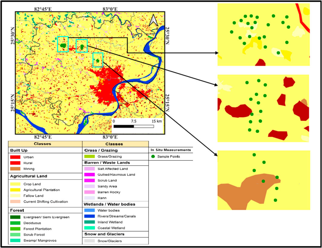
Figure 1. Geographical location of the test site (Source: Bhuvan WMS https://bhuvan-vec2.nrsc.gov.in/bhuvan/wms).

3 Methodology

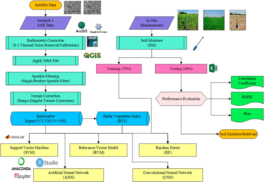
This study is centered on applying Sentinel 1 observations for soil moisture prediction in wheat fields. Wheat is a staple crop in this region, and its growth is highly dependent on irrigation availability at critical development stages. To ensure accurate and timely predictions, soil moisture data were collected on three specific dates during the wheat-growing season: 19th February, 9th March, and 14 April 2024 (Figure 2). These dates correspond to critical phenological stages of wheat growth, including tillering, flowering, and grain filling, where soil moisture is crucial in determining the final yield. Ground-based soil moisture measurements were obtained using the HydroGo device, a portable tool that measures soil moisture at a depth of 5 cm. These ground measurements provide a reliable reference for validating satellite-derived estimates (Entekhabi et al., 2010). Sentinel-1, a European Space Agency (ESA) satellite equipped with SAR, was utilised to acquire images on the exact dates. From these images, backscattering coefficients were extracted for ${\sigma }^{0}VV$ (vertical transmit and receive polarization), ${\sigma }^{0}VH$ (vertical transmit and horizontal receive polarization), ${\sigma }^{0}VV+{\sigma }^{0}VH$, and the Radar Vegetation Index (RVI). The use of RVI (Equation 1) is the replacement for NDVI which is crucial for vegetation health monitoring (Kumar et al., 2013). These backscattering values are sensitive to soil moisture and vegetation characteristics, making them suitable indicators for modeling soil moisture levels (Wagner et al., 2007).

$RVI=\frac{4*{\sigma }^{0}VH}{{\sigma }^{0}VV+{\sigma }^{0}VH}(1)$

Figure 2

Figure 2. Flowchart depicting the ML/DL-based soil moisture predictive modeling used in this study.

3.1 Data acquisition

3.1.1 In-Situ data acquisition

In-situ soil moisture (SM) was collected in the agricultural fields through HydraGO (a moisture measurement device for the upper soil layer). This device can get SM at depths of 5 cm, and in these places, sample readings get stored in an app called HydraGO, which Stevens Water Monitoring Systems, Inc. developed. It can also provide the latitude and longitude coordinates of the locations where the ground samples were read by accessing the mobile device’s GPS system. The SM samples are collected from 42 spatially different locations regularly monitored for three different crop growth stages, and measurements were done three times in three different months (February, March, and April). The HydraGO-based in situ soil moisture measurement had shown a fair correlation with the ground measurements (Wang et al., 2024), and it has lower uncertainties associated with the device (Murugesan et al., 2023).

3.1.2 SAR data acquisition and processing

The SAR Sentinel-1 data was taken from the Copernicus Data (https://dataspace.copernicus.eu/) for the proposed study area of three different months. The analysis was based on Sentinel-1 with polarizations (VV and VH). The pre-processing requires subsequent steps such as radiometric correction, thermal noise removal, calibration, apply orbit file, speckle filtering, geometric correction, and terrain correction. Afterwards, the backscattering was extracted by using Sentinel-1 pre-processed images of the study area and getting the backscattering coefficient of ${\sigma }^{0}VV$, ${\sigma }^{0}VH$, ${\sigma }^{0}VV+{\sigma }^{0}VH$. All these processes are done using software called SNAP version 10.0.0 (https://step.esa.int/main/download/snap-download/) (Moreira et al., 2013; Torres et al., 2012). The Radar Vegetation Index was then calculated by using the ${\sigma }^{0}VV$, ${\sigma }^{0}VH$, which showed a good relationship with SM by many researchers (Chaudhary et al., 2021; Srivastava et al., 2015).

However, other SAR satellite data, such as NovaSAR and RADARSAT, are limited for the studied region. NovaSAR is expensive and was not available for the in situ soil moisture collection data so it would represent nonconcurrent data. Thus, NovaSAR data is not preferred for studying. In the case of RADARSAT, it is no different from NovaSAR attributes for the region. Apart from the mentioned limitation, no freely accessed data matches the temporal and spatial coverage such as the Sentinel 1 data for the study area. The sentinel data provide short temporal resolution and are preferred for agriculture studies (Li et al., 2021; Srivastava et al., 2024).

3.1.3 Machine learning and deep learning algorithms

The main purpose of ML and DL models is to estimate SM using the backscattering data and RVI. Supervised machine learning models were used as they utilises training data or labelled data that are typically used in models to predict future values or events. In the present study, there are mainly five types of ML/DL were used: SVM, RVM, RF, ANN, and CNN, to estimate and predict the SM over the study area.

3.1.3.1 Support vector machine (SVM)

The SVM regression model uses an RBF kernel to predict soil moisture from satellite-derived radar backscatter measurements and the Radar Vegetation Index (RVI). Following the formulation found in (Cortes and Vapnik, 1995), the SVM model seeks to minimise the regularised risk function:

${\min }_{\mathrm{w},\mathrm{b},\mathrm{\xi },{\mathrm{\xi }}^{*}}\frac{1}{2}{‖\mathit{w}‖}^{2}c{\displaystyle \sum _{i=1}^n}\left({\mathrm{\xi }}_i+{\mathrm{\xi }}_i^{*}\right)(2)$

subject to:

${\mathrm{y}}_{\mathrm{i}}-\left(\mathbf{w}·\mathrm{\varphi }\left({\mathrm{x}}_{\mathrm{i}}\right)+\mathrm{b}\right)\le \epsilon +{\mathrm{\xi }}_i,(3)$

$\left(\mathbf{w}·\mathrm{\varphi }\left({\mathrm{x}}_{\mathrm{i}}\right)+\mathrm{b}\right)-{\mathrm{y}}_{\mathrm{i}}\le \epsilon +{\mathrm{\xi }}_i^{*},(4)$

${\mathrm{\xi }}_i,{\mathrm{\xi }}_i^{*}\ge 0\text{\hspace{0.17em}for\hspace{0.17em}all\hspace{0.17em}}\mathrm{i},(5)$

in Equation 2–5 the parameter w is the weight vector, b is the bias, ϕ (xi) represents the high-dimensional feature transformations, and ${\mathrm{\xi }}_i$, ${\mathrm{\xi }}_i^{*}$ are the slack variables (Cortes and Vapnik, 1995). The RBF kernel, described by (Schölkopf and Smola, 2002), alters the training data into a higher-dimensional space using the kernel function:

$K\left(x_i,x_j\right)=\mathit{exp}\left(-\gamma {\parallel x_i-x_j\parallel }^2\right),(6)$

in Equation 6, the γ is a parameter that defines the spread of the kernel and thus influences decision boundary’s smoothness and complexity (Schölkopf and Smola, 2002). The choice of the RBF kernel allows the SVM to handle the non-linear relationships often present in environmental data sets, a technique further discussed in (Cristianini, 2000). Parameter tuning, particularly the choice of CCC and γ, was guided by the practical insights provided in (Chang and Lin, 2011).

The SVM model’s hyperparameters was tuned with the radial basis function (RBF) kernel: the cost parameter (C) and the kernel parameter (gamma). The cost parameter was varied to establish an optimal balance between minimising error and reducing overfitting by penalising misclassified instances. The gamma parameter, which governs the influence of individual training samples, was adjusted to effectively capture the non-linear relationships between the predictors and soil moisture. To ensure a robust and reliable evaluation of the model, a five-fold cross-validation technique was utilised, allowing the model to be trained and tested on various subsets of the dataset.

3.1.3.2 Relevance Vector Machine (RVM)

This study employed a Relevance Vector Machine (RVM) for predicting soil moisture using a polynomial kernel. The RVM, an advanced machine learning technique based on Bayesian inference principles, offers a probabilistic counterpart to Support Vector Machines (SVM) with a key advantage in producing sparser solutions (Tipping, 2001). The model output, y(x), is defined by the linear combination of weights and high-dimensional features mappings, represented as

$y\left(x\right)=w^T\varphi \left(x\right)+ϵ,(7)$

in Equation 7, the w is the weight vector, $\varphi$ (x) denotes the kernel-induced feature space and $ϵ$ is Gaussian noise (Bishop, 2006).

The kernel function for the RVM was specified as a polynomial kernel,

$K\left(x_i,x_j\right)={\left(1+\left(x_i,x_j\right)\right)}^2,(8)$

in Equation 8, where d is the polynomial degree, enhancing ability of the model to capture non-linear relationships in environmental data (Schölkopf and Smola, 2002). Learning in RVM involves maximising marginal likelihood of the observed data, and integrates over the weights, formulated as the following equation:

$p\left(w\left|t,X,\alpha ,{\sigma }^2)\propto p(t\right|X,w,{\sigma }^2\right)p\left(w|\alpha \right),(9)$

in Equation 9, where t and X are targets and input vectors, respectively, α are hyperparameters including sparsity, and σ² is the noise variance (Tipping, 2001).

RVM’s preference for sparsity is facilitated through Automatic Relevance Determination (ARD), which drives many weight parameters towards zero, effectively reducing the model’s complexity while retaining predictive accuracy. This aspect is crucial in determining the relevance vectors, which are instrumental in the model’s training and prediction phases (Bishop, 2006).

A Relevance Vector Machine (RVM) was fine-tuned for soil moisture prediction using Sentinel-1 parameters, leveraging a polynomial kernel to model nonlinear relationships. Input features were normalised, and hyperparameters, including kernel degree and regularisation, were optimised via grid search. Five-fold cross-validation ensured robust generalisation, while metrics like RMSE and R-squared confirmed high prediction accuracy. The model achieved minimal bias and strong alignment between observed and predicted values, making it a reliable tool for soil moisture monitoring in agriculture.

3.1.3.3 Random Forest (RF)

The Random Forest was employed to predict soil moisture, leveraging its capacity to manage large datasets characterized by complex, non-linear interactions among variables. RF is an ensemble learning method developed by Leo Breiman. The RF model constructs a multitude of decision trees at training time, and the result is the mean prediction of the individual trees that produce the model prediction. This method is particularly effective due to its intrinsic ability to reduce variance without increasing bias significantly, thus mitigating the overfitting problem prevalent in single decision trees (Breiman, 2001).

The trees in the forest are generated from a unique bootstrap sample, drawing randomly with replacement from the training dataset, thus ensuring that each tree learns from a slightly different subset of the data. This approach is known as bootstrap aggregating or bagging and it increases the diversity among the trees in the model, which is crucial for achieving robustness in the predictions (Equation 10):

$D_i=\left(x^{\left(i\right)},y^{\left(i\right)}\right),\dots ..,\left(x_n^{\left(i\right)},y_n^{\left(i\right)}\right)(10)$

For each node of trees, the algorithm selects a random subset of the features. It determines the best split based on minimizing the sum of the squared residuals, thereby ensuring that each split contributes effectively to reducing the overall prediction error (Equation 11):

$j^{*},t^{*}={\arg \mathit{min}}_{j,t}\left[{\mathit{min}}_{c1}{\displaystyle \sum _{x_i\in R_1\left(j,t\right)}}{\left(y_i-c_1\right)}^2+{\mathit{min}}_{c2}{\displaystyle \sum _{x_i\in R_2\left(j,t\right)}}{\left(y_i-c_2\right)}^2\right](11)$

The predictions from all trees are then aggregated to determine the final prediction by averaging, which significantly reduces the variance while retaining the bias low (Equation 12):

$\widehat{y}\left(x\right)=\frac{1}{B}{\displaystyle \sum _{i=1}^B}{t}_i\left(x\right)(12)$

where B denotes the number of trees. This aggregation helps in canceling out errors across the different trees, leading to more accurate and stable predictions, especially in complex environmental applications such as soil moisture prediction where the inputs might have high variability and inter-correlations (James et al., 2013).

The Random Forest algorithm’s ability to handle high-dimensional spaces and maintain accuracy even when most predictive variables have noise significantly enhances its suitability for ecological and hydrological modeling. It is adept at capturing essential patterns in the data, which could be missed by simpler models, thus providing a profound tool for predicting phenomena that depend on subtle environmental cues.

The Random Forest (RF) model was fine-tuned to optimise its predictive performance, using 500 decision trees to balance computational efficiency and accuracy. The mtry parameter, representing the number of predictors considered at each split, was set to 2 based on extensive cross-validation, enhancing model diversity and reducing overfitting. A 5-fold cross-validation approach was employed for robust evaluation, ensuring unbiased performance estimates on unseen data. This tuning process significantly improved the RF model’s ability to predict soil moisture, effectively capturing the relationship between Sentinel-1 backscatter parameters and soil moisture with high accuracy and strong generalizability.

3.1.3.4 Artificial Neural Network (ANN)

The ANN model was employed to predict soil moisture, leveraging its ability to model complex, and non-linear relationships inherent in environmental data. ANNs are computational systems inspired by the neural structures of the human brain, consisting of interconnected layers of nodes or neurons. Each neuron processes input through weighted sums and a non-linear activation function, enabling the network to capture intricate patterns from the input features (Haykin, 1998).

During the training phase, the ANN adjusts its internal weights through backpropagation, an optimization technique that iteratively updates the weights to reduce the discrepancy between predicted and actual outputs (Rumelhart et al., 1986). The equation defined the linear output of the network:

$y=f\left(W.x+b\right)(13)$

in Equation 13, where x represents the input features, W the weight matrix, b the bias vector, and f the linear transformation function.

Performance metrics such as RMSE, R-squared, and the correlation coefficient were calculated to assess the model’s accuracy. The statistical metrics offer an assessment of the model’s capacity to accurately approximate the actual soil moisture values from radar backscatter measurements and RVI, demonstrating the effectiveness of the ANN in environmental data analysis (Chollet and Allaire, 2018). Furthermore, feature scaling was implemented as a preprocessing measure to ensure that all input variables contributed equitably to the model training. This step is crucial in neural network models to prevent the dominance of features with larger-scale values, ensuring a balanced and effective learning process (Goodfellow, 2016).

The ANN model for soil moisture prediction was optimised by tuning the number of hidden layer neurons (5–10) and the regularisation decay parameter (0.1 and 0.01) to balance complexity and generalisation. Three-fold cross-validation ensured robust evaluation, and input features were standardised for consistent learning. This systematic tuning achieved high prediction accuracy and reliable performance on both training and testing datasets.

3.1.3.5 Convolution neural network (CNN)

The CNN model has been employed to predict soil moisture, exploiting its ability to process spatial data effectively. CNNs, known for their hierarchical feature extraction, excel at capturing complex patterns in satellite imagery, making them ideal for environmental applications such as soil moisture estimation. The CNN architecture was implemented using the “Keras” library, consisting of multiple sequential layers explicitly designed for feature extraction and regression analysis. The initial convolutional layer was equipped with 32 filters of size 1 × 3 and utilised the Rectified Linear Unit as an activation function. This layer is critical for extracting spatial features from the input data, with the convolution operation expressed mathematically as (Equation 14):

$a^{\left[l\right]}=g\left(W^{\left[l\right]}*x^{\left[l-1\right]}+b^{\left[l\right]}\right)(14)$

where a [l] represents the activation at layer l, W [l]and b [l] are the weights and biases, x [l−1] is the input from the previous layer, ∗ denotes the convolution operation, and g is the Rectified Linear Unit function that introduces non-linearity (LeCun et al., 1998).

Furthermore, a max pooling layer with a pool size of 1 × 2 reduced the spatial dimensions of the feature maps. This pooling operation simplifies the output by only passing the maximum value from each region of the feature map, as described by (Equation 15):

$a_{ij}^{\left[l\right]}={\mathit{max}}_{p,q\in region}{a}_{pq}^{\left[l-1\right]}(15)$

This reduces computational load while retaining essential features crucial for controlling overfitting (Scherer et al., 2010).

Further layers included another convolutional layer with 64 filters of the same size to deepen the network’s capacity to discern more complex environmental patterns. The network then employed a flattening step that converts the multidimensional feature maps into a one-dimensional feature vector, which was subsequently passed through a fully connected dense layer with 50 Rectified Linear Units. This culminated in a regression output layer to predict continuous soil moisture values. The model was trained using the RMSprop optimiser, an adaptive learning rate technique particularly effective for deep learning tasks involving large data sets (Tieleman, 2012).

A GPU-accelerated CNN was developed for soil moisture prediction, featuring optimized convolutional and dense layers with ReLU activation and max-pooling. Key hyperparameters, including RMSprop optimizer, batch size, and 40,000 epochs, were fine-tuned. Input normalisation and a 20% validation split ensured robust performance, with metrics like RMSE confirming accurate predictions from Sentinel-1 features.

4 Results and discussion

4.1 Analysis of the in situ datasets and backscattering

The Soil Moisture, ${\sigma }^{0}VV$, ${\sigma }^{0}VH$, ${\sigma }^{0}VV+{\sigma }^{0}VH$, and RVI box plots clearly displayed the distribution and variability at different dates. Each plot brings out the median, interquartile range, and outliers that may indicate peculiar conditions or measurement anomalies. The SM box plot shows variation in soil moisture over time; wider boxes show more significant variability, while outliers indicate some specific locations with entirely different moisture values. Likewise, ${\sigma }^{0}VV$ and ${\sigma }^{0}VH$ box plots show how radar backscatter behaves for different surface variables. The plot for RVI provides information on vegetation dynamics with changes in median values, indicating changes in vegetation cover or structure. In general, the box plots add significantly to understanding the temporal patterns and space variability of the parameters under study, such as environmental situations during that period. The in situ soil moisture variability and relation have been captured by ${\sigma }^{0}VH\text{\hspace{0.17em}and\hspace{0.17em}RVI}$. These two variables (${\sigma }^{0}VH$ and RVI) become a feature of importance and have a higher weight in the prediction of soil moisture in comparison to ${\sigma }^{0}VV$ and ${\sigma }^{0}VV+{\sigma }^{0}VH$. Therefore, box plots of in situ soil moisture and machine learning features improve the decision-making in feature engineering by a modular. This enables us to improve the prediction capabilities of models used in the study (Figure 3).

Figure 3

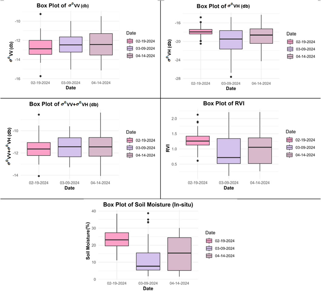
Figure 3. Box and whisker Plots of ${\sigma }^0$ VV, ${\sigma }^0$ VH ${\sigma }^0$ VV+ ${\sigma }^0$ VH, RVI and in situ SM data for three crop growth stages.

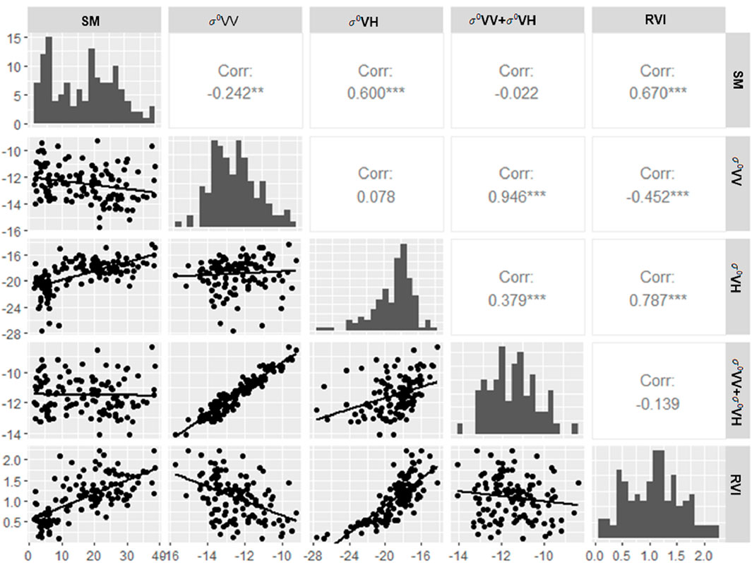
The scatterplot matrix (Figure 4) illustrates the relationships between soil moisture (SM) and various radar-derived parameters and derived index, including ${\sigma }^{0}VV$, ${\sigma }^{0}VH$, ${\sigma }^{0}VV+{\sigma }^{0}VH$, and RVI. Each cell presents a scatterplot showing the relation of variables among each other with their corresponding correlation coefficients. In (Figure 4), the correlation values are accompanied by significance level indicators: (*) denotes that the observed relationship is unlikely to have occurred by chance, with a confidence level of 95%. Additionally, (**) indicates a 99% confidence that the relationship is not attributable to random variation. Finally, (***) suggests solid evidence against the null hypothesis, boasting a confidence level of 99.9%. These markers effectively convey the significance levels in a concise manner. SM showed is a weak negative correlation (−0.242) with ${\sigma }^{0}VV$, indicating that higher soil moisture slightly reduces the backscatter in the VV polarisation. This relationship is statistically significant at the 0.01 level. In contrast, SM shows a moderate positive correlation (0.600) with ${\sigma }^{0}VH$, suggesting that increases in soil moisture can be associated with higher backscatter in the VH polarisation. This correlation is highly significant, indicating a strong relationship. Meanwhile, there is almost no correlation (−0.022) between SM and ${\sigma }^{0}VV+{\sigma }^{0}VH$, implying that the combined backscatter from both polarisations does not directly reflect changes in soil moisture. However, SM has a strong positive correlation (0.670) with RVI, suggesting a close relationship between soil moisture levels and vegetation conditions. The selection of indices ${\sigma }^0\text{\hspace{0.17em}VV}+{\sigma }^0\text{\hspace{0.17em}VH}$ is based on its ability to incorporate the soil moisture conditions and the wheat growth stages. A previous study found that the use of ${\sigma }^0$ VV+ ${\sigma }^0$ VH indices was highly correlated with canopy coverage (Nasirzadehdizaji et al., 2019). Thu, ${\sigma }^0\text{\hspace{0.17em}VV}+{\sigma }^0\text{\hspace{0.17em}VH}$ indices used in the current approach ensure the soil moisture conditions through VV polarisation and plant canopy coverage for agricultural through ${\sigma }^0\text{\hspace{0.17em}VV}+{\sigma }^0\text{\hspace{0.17em}VH}$. Additionally, trained model applications on satellite imagery help to follow the wheat crop extant for soil moisture conditions. It is crucial to note that the models are trained using 1D models; hence, keeping the ${\sigma }^0\text{\hspace{0.17em}VV}+{\sigma }^0\text{\hspace{0.17em}VH}$ parameter limits the predictions on satellite images (2D) over crop extent. Since we have not used optical indices like NDVI in the model training, the ${\sigma }^0\text{\hspace{0.17em}VV}+{\sigma }^0\text{\hspace{0.17em}VH}$ becomes important to train the model for agricultural areas. Overall, the scatterplot matrix reveals several important relationships. Strong correlations, such as those between SM and ${\sigma }^{0}VH$, and SM and RVI, suggest that these parameters could serve as effective predictors for soil moisture. Conversely, the weak correlations (e.g., SM with ${\sigma }^{0}VV+{\sigma }^{0}VH$) imply limited predictive value. These insights are valuable for developing models that leverage radar-derived data to monitor soil moisture and vegetation health, particularly for agricultural and environmental applications.

Figure 4

Figure 4. Soil moisture (in situ) relationship among the SAR backscattering and derived features.

SM and backscattering relationship are valuable for developing improved prediction models that leverage radar-derived data, which can be especially beneficial for applications in agriculture, water management, and environmental monitoring. Understanding these patterns is crucial for enhancing the accuracy of soil moisture prediction models. Changes in soil moisture can influence radar backscatter and vegetation indices, reflecting varying soil and vegetation conditions. In (Figure 5), SM is compared with ${\sigma }^{0}VV$. The left y-axis represents soil moisture as a percentage, while the right y-axis shows the backscatter coefficient in decibels (dB). The SM trend indicates a decline from 19 February to 09 March, followed by a slight increase on 14 April maybe due to irrigation provided to the field. The ${\sigma }^{0}VV$, on the other hand, exhibit an opposite pattern: they rise between February and March and then drop slightly by April. This inverse relationship suggests that higher soil moisture may cause lower backscattering, resulting in reduced backscatter (lower ${\sigma }^{0}VV$), while drier conditions reflect more radar signals, increasing the backscatter coefficient. The bottom left graph plots SM against ${\sigma }^{0}VH$. Similar to the previous graph, the SM shows a decline from February to March, followed by a rise in April. However, ${\sigma }^{0}VH$ shows a downward trend from February to March, reaching its lowest point, and then increasing in the April. This indicates a more complex interaction between soil moisture and the VH polarization, suggesting that changes in soil moisture have varying effects on radar backscattering, depending on the polarization mode. A lower ${\sigma }^{0}VH$ might imply that, during wetter conditions, there is less scattering, while drier soil contributes to higher backscattering values. To understand the variation between SM and RVI, soil moisture (SM) is plotted alongside the RVI. The RVI, displayed on the right y-axis, mirrors this trend, decreasing between February and March and then rising slightly in April. This parallel pattern suggests a correlation between soil moisture levels and vegetation conditions, where reduced soil moisture corresponds to lower RVI values, potentially indicating a decline in vegetation health during drier periods. The bottom right graph compares soil moisture (SM) to ${\sigma }^{0}VV+{\sigma }^{0}VH$, a backscatter coefficient measured in decibels (dB). Here, an inverse trend is observed: as soil moisture decreases from February to March, ${\sigma }^{0}VV+{\sigma }^{0}VH$ also drops, but it increases again in April when soil moisture levels rise. This behavior implies a complex interaction between radar backscatter and soil moisture. Typically, higher soil moisture may lead to greater absorption of radar signals, resulting in lower backscattering values, while vice versa for the drier conditions. The graphs illustrate a dynamic relationship between soil moisture and radar backscattering coefficients in both VV and VH polarizations, as well as the connection between soil moisture and vegetation indices derived from radar data.

Figure 5

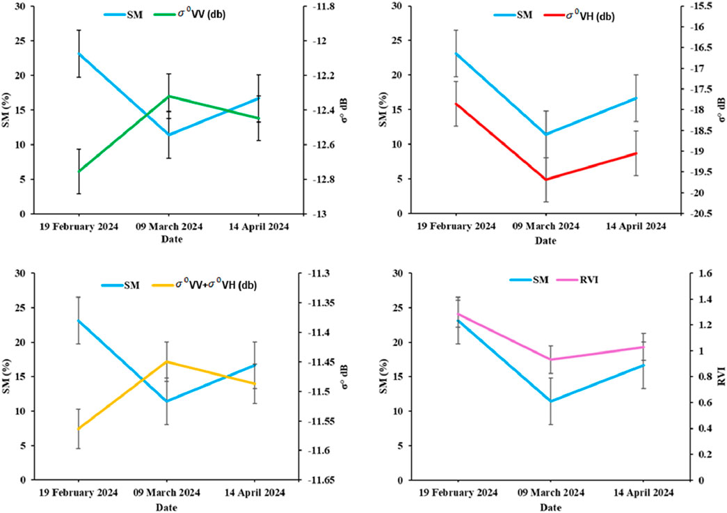
Figure 5. Temporal variations between in situ soil moisture and spatially averaged backscattering and SAR data derived parameters.

4.2 Performance evaluation of the ML/DL

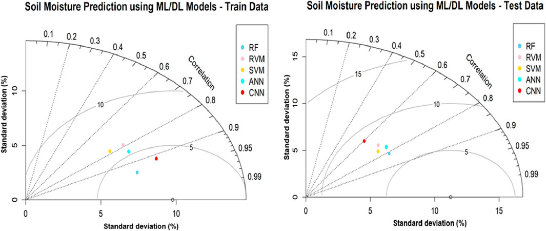
Taylor diagrams (Figure 6) illustrated the performance of various ML/DL models in predicting soil moisture, which was evaluated across both training and testing datasets. These diagrams determine three critical statistics: the correlation coefficient, standard deviation, and centred root mean square difference (RMSD) relative to observed data. The model’s correlation coefficient shows the metric represented by the angular displacement of each model’s marker from the reference point, which denotes perfect agreement with the observations. It is particularly noticeable in models such as SVM and CNN, which exhibit greater unpredictability and deviations in error measures, even though they preserve strong correlation coefficients with the observed data. The standard deviation was illustrated by the radial distance, which was from the origin; this metric measures the model’s output variability compared to that of the observations of the models. A model’s output that matches the observed standard deviation will lie on the circle marked with the observed standard deviation data. The centred RMSD, depicted by the distance from each model’s marker to the reference point. The less distance suggests that a model’s predictions are closer to the observed values. The diagrams of the training dataset reveal that a simpler model, RF, aligns closely with the reference point, demonstrating both high correlation and comparable variability to the observed data. These models also show lower RMSD, indicating high accuracy in learning from train data. In the test dataset, models exhibit a broader dispersion of markers, reflecting varied performance. Despite maintaining decent correlation coefficients, some models increased standard deviations, and RMSDs highlight difficulties in generalising learned patterns to new data. This is notably evident in models like SVM and CNN, which, while maintaining good correlations, show more significant variability and error metrics deviations. The analysis of the Taylor diagrams provides critical insights into the behavior of various models under different data conditions. Less complex model RF tends to be more robust, possibly due to their lower propensity for overfitting than more complicated models like SVM and CNN. This observation is crucial for model selection, emphasising the need to balance capturing complex patterns and maintaining generalizability across datasets.

Figure 6

Figure 6. Taylor plots representing the Performance of ML/DL Models.

4.3 Statistical evaluation of ML/DL models

The first model (ANN) showed a strong fit, with an RMSE of 5.46, a correlation of 0.83, and negligible bias on training data. Testing results reported an RMSE of 7.66 and a correlation of 0.77, though a bias of −2.32 indicated a slight underestimation. The ANN demonstrated effective soil moisture prediction capabilities, suggesting its value for environmental studies. On training the second model, the CNN achieved an RMSE of 3.9, an R-squared of 0.84, and a correlation coefficient of 0.92, with a minimal bias of 0.71, demonstrating strong performance and robust pattern recognition. Testing results exhibit an RMSE of 8.44, an R-squared of 0.43, and a correlation of 0.67, with a bias of −1.39, indicating underestimation. Despite declining testing data accuracy, the model effectively generalizes and maintains consistent prediction patterns. The third (RF) model performed exceptionally well on training data, with an RMSE of 3.44, an R-squared of 0.88, and a correlation coefficient 0.95. Minimal bias (−0.04) indicated high precision. However, testing results showed a decline, with an RMSE of 7.06, R-squared of 0.61, and a correlation of 0.8, alongside a bias of −1.64, suggesting underestimation. Despite these limitations, the RF model’s strong performance in training highlights its capacity to capture nonlinear relationships, though improvements may be necessary to enhance generalisation. The second last (RVM) model achieved an RMSE of 6.13, an R-squared of 0.61, and a correlation of 0.78 on training data, with minimal bias (0.37). In testing, the model-maintained performance with an RMSE of 8.58, an R-squared of 0.51, and a slight underestimation bias of 3.36, suggesting effective generalisation for soil moisture estimation using radar backscatter data. The last SVM model reported an RMSE of 6.04 and an R-squared of 0.62 on training data, with a correlation coefficient of 0.79 and a minor bias of 0.29. For testing data, RMSE rose to 7.92, R-squared dropped to 0.5, and the correlation reduced to 0.73, with a bias of −1.99. These results demonstrate the SVM’s capability, though challenges remain in generalising across varied datasets, underscoring the importance of model complexity and continuous adaptation.

As shown in Table 1, the above-based model’s metrics performance, the RF model provided the best-performing model for soil moisture prediction, demonstrating superior accuracy on the training data. In contrast, the testing data showed some performance degradation, but the model still maintained a reasonable level of accuracy. Therefore, the RF stands out as the competent model, providing a strong balance of accuracy, robustness, and generalisation, making it suitable for practical applications in soil moisture monitoring. Future enhancements could include additional data preprocessing, feature selection, or tuning to further minimize errors and improve prediction accuracy in real-world scenarios.

Table 1

Table 1. Statistical comparison between the ML and DL models used in the study.

4.4 Assessment of over/underfitting of the model

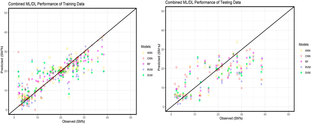
The one-to-one plots depicted here are essential tools in which they could evaluate the over/underfitting of ML and DL models specifically, which were applied to predict soil moisture prediction (Srivastava et al., 2014). These plots are structured to compare the predicted soil moisture values against the observed data across two trained and tested datasets. The one-to-one line, represented by a solid black line, served as a benchmark for perfect predictions, where an exact alignment of predicted values with the observed values would fall on this line, symbolising the model’s ideal performance. In the training section of the data plot (Figure 7), we observe a closer clustering of data points plotted in a one-to-one line across various models, including RF, RVM, SVM, ANN, and CNN. This clustering shows a high degree of accuracy during the training phase, which suggests that these models have effectively learned and replicated the underlying patterns in the training dataset. The proximity of predictive measures to the one-to-one line indicates minimal deviation from observed values, reflecting a solid internal validation of model predictions during training. Also, the testing data plot reveals a broader spread of points away from the one-to-one line, highlighting the models’ challenges in generalising unseen data. The spread of predictive measures shows variability in the model’s performance, with some models showing substantial deviations from the observed data. Such variability underscores the complex nature of model behaviour outside controlled environments, revealing discrepancies in model predictions when applied in practical scenarios. This divergence is crucial for understanding each model’s reliability and generalisation capabilities, guiding further model refinement. The analysis of both plots emphasises the necessity for ongoing assessment and optimisation of predictive models to enhance their accuracy and reliability in real-world applications, particularly in environmental and agricultural planning where precise soil moisture estimation is critical.

Figure 7

Figure 7. Combined machine/deep learning (ML/DL) performance of training and testing data.

4.5 Spatial prediction of soil moisture through the best model

The predictions are visualised through raster images derived from processed Sentinel-1 data, incorporating features such as ${\sigma }^{0}VV$, ${\sigma }^{0}VH$, ${\sigma }^{0}VV+{\sigma }^{0}VH$, and RVI. Each map employs a colour scale ranging from blue to yellow, indicating low and high soil moisture levels. The progression of dates shows changes in soil moisture distribution influenced by seasonal climatic conditions. This approach provides soil moisture levels at the spatial scale. The transformation of in situ measurements at a specific location turned into a continuous soil moisture raster image, and the algorithm’s ability to capture the dynamic changes in the predicted soil moisture illustrates machine learning and deep learning applications in efficient agriculture or irrigation planning (Figure 8).

Figure 8

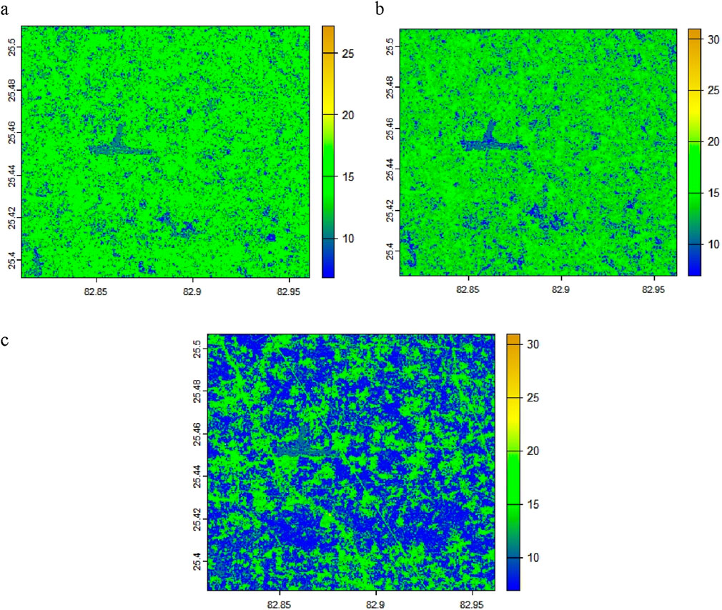
Figure 8. Soil Moisture (%) mapping using the best model, i.e., RF at different stages: (A) 19th February, (B) 09th March (C) 14 April 2024.

5 Conclusion

The current study successfully demonstrated the potential of ML and DL models in predicting soil moisture levels from Synthetic Aperture Radar (SAR) data in the wheat fields. The study showcased the benefits of integrating satellite remote sensing with ML and DL algorithms techniques for agricultural applications by combining rigorous data collection with innovative computational methods. Evaluating models such as SVM, RVM, RF, ANN, and CNN revealed unique strengths in capturing soil moisture dynamics. The Random Forest model emerged as a top performer in the training and testing phases, highlighting its ability to handle complex environmental datasets. Meanwhile, deep learning models like Convolutional Neural Networks leveraged their architectural features to analyse spatial patterns in SAR data, although with varying degrees of success across different testing scenarios. This research improved the accuracy of soil moisture predictions and can contribute to the development of precision agriculture in the region by enhancing irrigation strategies and water resource management. It emphasised the importance of continuous monitoring and model updating to adapt to changing environmental conditions and agricultural practices. Integrating remote sensing data with machine learning and deep learning approaches holds promise for scaling these technologies to other regions and crop types, potentially transforming agricultural practices globally. Future studies could build upon this work by incorporating diverse data sources and refining model architectures to improve the generalizability and accuracy of soil moisture predictions. Ultimately, this study provides a scalable, cost-effective solution for near real-time soil moisture monitoring, promoting sustainable agricultural practices crucial for food security and resource management in the face of increasing climate variability.

Data availability statement

The raw data supporting the conclusions of this article will be made available by the authors, without undue reservation.

Author contributions

DL: Formal Analysis, Investigation, Methodology, Software, Validation, Visualization, Writing–original draft, Writing–review and editing. SP: Investigation, Software, Visualization, Writing–original draft, Writing–review and editing. PS: Conceptualization, Funding acquisition, Methodology, Project administration, Resources, Supervision, Writing–original draft, Writing–review and editing. SS: Resources, Visualization, Writing–original draft, Writing–review and editing. MG: Data curation, Project administration, Resources, Supervision, Writing–original draft, Writing–review and editing. RP: Resources, Software, Writing–original draft, Writing–review and editing.

Funding

The author(s) declare that financial support was received for the research, authorship, and/or publication of this article. We are thankful to the RESPOND/ISRO and Institute of Eminence, Banaras Hindu University for providing the necessary funding for this research.

Conflict of interest

The authors declare that the research was conducted in the absence of any commercial or financial relationships that could be construed as a potential conflict of interest.

Generative AI statement

The author(s) declare that no Generative AI was used in the creation of this manuscript.

Publisher’s note

All claims expressed in this article are solely those of the authors and do not necessarily represent those of their affiliated organizations, or those of the publisher, the editors and the reviewers. Any product that may be evaluated in this article, or claim that may be made by its manufacturer, is not guaranteed or endorsed by the publisher.

References

Anand, A., Pandey, M. K., Srivastava, P. K., Gupta, A., and Khan, M. L. (2021). Integrating multi-sensors data for species distribution mapping using deep learning and envelope models. Remote Sens. 13 (16), 3284. doi:10.3390/rs13163284

CrossRef Full Text | Google Scholar

Barrett, B., and Petropoulos, G. P. (2013). Satellite remote sensing of surface soil moisture. Remote Sens. Energy Fluxes Soil Moisture Content 85, 85–119. doi:10.1201/b15610

CrossRef Full Text | Google Scholar

Bishop, C. M. (2006). Pattern recognition and machine learning. Springer Google Sch. 2, 1122–1128.

Google Scholar

Breiman, L. (2001). Random forests. Mach. Learn. 45, 5–32. doi:10.1023/a:1010933404324

CrossRef Full Text | Google Scholar

Brocca, L., Ciabatta, L., Moramarco, T., Ponziani, F., Berni, N., and Wagner, W. (2016). “Use of satellite soil moisture products for the operational mitigation of landslides risk in central Italy,” in Satellite soil moisture retrieval (Elsevier), 231–247.

CrossRef Full Text | Google Scholar

Chang, C.-C., and Lin, C.-J. (2011). LIBSVM: a library for support vector machines. ACM Trans. Inte. Syst. Technol. (TIST) 2 (3), 1–27. doi:10.1145/1961189.1961199

CrossRef Full Text | Google Scholar

Chaudhary, S. K., Gupta, D. K., Srivastava, P. K., Pandey, D. K., Das, A. K., and Prasad, R. (2021). Evaluation of radar/optical based vegetation descriptors in water cloud model for soil moisture retrieval. IEEE Sensors J. 21 (18), 21030–21037. doi:10.1109/jsen.2021.3099937

CrossRef Full Text | Google Scholar

Chaudhary, S. K., Srivastava, P. K., Gupta, D. K., Kumar, P., Prasad, R., Pandey, D. K., et al. (2022). Machine learning algorithms for soil moisture estimation using Sentinel-1: model development and implementation. Adv. Space Res. 69 (4), 1799–1812. doi:10.1016/j.asr.2021.08.022

CrossRef Full Text | Google Scholar

Chollet, F., and Allaire, J. (2018). Deep learning with R. Shelter Island, NY: Manning Publications Co.

Google Scholar

Cortes, C., and Vapnik, V. (1995). Support-vector networks. Mach. Learn. 20, 273–297. doi:10.1007/bf00994018

CrossRef Full Text | Google Scholar

Cristianini, N. (2000). An Introduction to Support Vector Machines and other kernel-based learning methods. Cambridge University Press.

Google Scholar

Duarte, E., and Hernandez, A. (2024). A review on soil moisture dynamics monitoring in semi-arid ecosystems: methods, techniques, and tools applied at different scales. Appl. Sci. 14 (17). doi:10.3390/app14177677

CrossRef Full Text | Google Scholar

Entekhabi, D., Njoku, E. G., O'neill, P. E., Kellogg, K. H., Crow, W. T., Edelstein, W. N., et al. (2010). The soil moisture active passive (SMAP) mission. Proc. IEEE 98 (5), 704–716. doi:10.1109/jproc.2010.2043918

CrossRef Full Text | Google Scholar

Foley, J. A., Ramankutty, N., Brauman, K. A., Cassidy, E. S., Gerber, J. S., Johnston, M., et al. (2011). Solutions for a cultivated planet. Nature 478 (7369), 337–342. doi:10.1038/nature10452

PubMed Abstract | CrossRef Full Text | Google Scholar

Goodfellow, I. (2016). Deep learning, 196. MIT press.

Google Scholar

Haykin, S. (1998). Neural networks: a comprehensive foundation. United States: Prentice Hall PTR.

Google Scholar

Inoubli, R., Constantino-Recillas, D. E., Monsiváis-Huertero, A., Farah, L. B., and Farah, I. R. (2024). “Computational methods to retrieve soil moisture using remote sensing data: A review,” in 2024, IEEE 7th International conference on advanced technologies, signal and image processing (ATSIP) 1, 77–82. doi:10.1109/ATSIP62566.2024.10638854

CrossRef Full Text | Google Scholar

Jackson, T., and Schmugge, T. (1991). Vegetation effects on the microwave emission of soils. Remote Sens. Environ. 36 (3), 203–212. doi:10.1016/0034-4257(91)90057-d

CrossRef Full Text | Google Scholar

James, G., Witten, D., Hastie, T., and Tibshirani, R. (2013). An introduction to statistical learning, 112. Springer.

Google Scholar

Kannan, A., Tsagkatakis, G., Akbar, R., Selva, D., Ravindra, V., Levinson, R., et al. (2022). “Forecasting soil moisture using a deep learning model integrated with passive microwave retrieval,” in Paper presented at the IGARSS 2022-2022 IEEE International Geoscience and Remote Sensing Symposium, Kuala Lumpur, Malaysia, 17-22 July 2022, 6112–6114. doi:10.1109/igarss46834.2022.9883245

CrossRef Full Text | Google Scholar

Kumar, D., Rao, S., and Sharma, J. (2013). “Radar Vegetation Index as an alternative to NDVI for monitoring of soyabean and cotton,” in Paper presented at the proceedings of the XXXIII INCA international congress (Indian cartographer) (India: Jodhpur).

Google Scholar

LeCun, Y., Bottou, L., Bengio, Y., and Haffner, P. (1998). Gradient-based learning applied to document recognition. Proc. IEEE 86 (11), 2278–2324. doi:10.1109/5.726791

CrossRef Full Text | Google Scholar

Li, Y., Zhang, C., and Heng, W. J. W. (2021). Retrieving surface soil moisture over wheat-covered areas using data from Sentinel-1 and Sentinel-2. Atmos. Sci. Meteo. 13(14), 1981. doi:10.3390/w13141981

CrossRef Full Text | Google Scholar

Mladenova, I., Jackson, T., Njoku, E., Bindlish, R., Chan, S., Cosh, M., et al. (2014). Remote monitoring of soil moisture using passive microwave-based techniques—theoretical basis and overview of selected algorithms for AMSR-E. Remote Sens. Environ. 144, 197–213. doi:10.1016/j.rse.2014.01.013

CrossRef Full Text | Google Scholar

Moreira, A., Prats-Iraola, P., Younis, M., Krieger, G., Hajnsek, I., and Papathanassiou, K. P. (2013). A tutorial on synthetic aperture radar. IEEE Geo. Rem. Sens. Mag. 1 (1), 6–43. doi:10.1109/mgrs.2013.2248301

CrossRef Full Text | Google Scholar

Murugesan, A., Dave, R., Kushwaha, A., Pandey, D. K., and Saha, K. J. J. o. A. (2023). Surface soil moisture estimation in bare agricultural soil using modified Dubois model for Sentinel-1 C-band SAR data. J. Agrometeorol. 25 (4), 517–524. doi:10.54386/jam.v25i4.2303

CrossRef Full Text | Google Scholar

Nasirzadehdizaji, R., Balik Sanli, F., Abdikan, S., Cakir, Z., Sekertekin, A., and Ustuner, M. J. A. S. (2019). Sensitivity analysis of multi-temporal Sentinel-1 SAR parameters to crop height and canopy coverage. Appl. Sci. (Basel). 9 (4), 655. doi:10.3390/app9040655

CrossRef Full Text | Google Scholar

Ray, S., and Majumder, S. (2024). Water Management in Agriculture: Innovations for Efficient Irrigation, 169–185.

Google Scholar

Roberts, T. M., Colwell, I., Chew, C., Lowe, S., and Shah, R. J. R. S. (2022). A deep-learning approach to soil moisture estimation with GNSS-R. Remote Sens. (Basel). 14 (14), 3299. doi:10.3390/rs14143299

CrossRef Full Text | Google Scholar

Robock, A., Vinnikov, K. Y., Srinivasan, G., Entin, J. K., Hollinger, S. E., Speranskaya, N. A., et al. (2000). The global soil moisture data bank. Bull. Am. Mete. Soc. 81 (6), 1281–1299. doi:10.1175/1520-0477(2000)081<1281:tgsmdb>2.3.co;2

CrossRef Full Text | Google Scholar

Rumelhart, D. E., Hinton, G. E., and Williams, R. J. (1986). Learning representations by back-propagating errors. Nature 323 (6088), 533–536. doi:10.1038/323533a0

CrossRef Full Text | Google Scholar

Scherer, D., Müller, A., and Behnke, S. (2010). “Evaluation of pooling operations in convolutional architectures for object recognition,” in Paper presented at the International conference on artificial neural networks (Springer, Berlin, Heidelberg: Lecture Notes in Computer Science).

Google Scholar

Schölkopf, B., and Smola, A. J. (2002). Learning with kernels: support vector machines, regularization, optimization, and beyond. MIT press.

Google Scholar

Singh, R., Srivastava, P. K., Petropoulos, G. P., Shukla, S., and Prasad, R. (2022). Improvement of the triangle method for soil moisture retrieval using ECOSTRESS and sentinel-2: results over a heterogeneous agricultural field in northern India. Water 14 (19), 3179. doi:10.3390/w14193179

CrossRef Full Text | Google Scholar

Singh, S. K., Prasad, R., Srivastava, P. K., Yadav, S. A., Yadav, V. P., and Sharma, J. (2023). Incorporation of first-order backscattered power in water cloud model for improving the leaf area index and soil moisture retrieval using dual-polarized sentinel-1 SAR data. Remote Sens. Environ. 296, 113756. doi:10.1016/j.rse.2023.113756

CrossRef Full Text | Google Scholar

Soothar, R. K., Singha, A., Soomro, S. A., Chachar, A., Kalhoro, F., and Rahaman, M. A. (2021). Effect of different soil moisture regimes on plant growth and water use efficiency of Sunflower: experimental study and modeling. Bull. Natl. Res. Centre 45 (1), 121. doi:10.1186/s42269-021-00580-4

CrossRef Full Text | Google Scholar

Srivastava, H. S., Sivasankar, T., Gavali, M. D., and Patel, P. J. K. J. o. S. (2024). Soil moisture estimation underneath crop cover using high incidence angle C-band Sentinel-1 SAR data. Kuwait J. Sci. 51 (1), 100101. doi:10.1016/j.kjs.2023.07.007

CrossRef Full Text | Google Scholar

Srivastava, P., O'Neill, P., Cosh, M., Lang, R., and Joseph, A. (2015). “Evaluation of radar vegetation indices for vegetation water content estimation using data from a ground-based SMAP simulator,” in TU2.Y1: soil moisture algorithms and downscaling (Milan, Italy: IGARSS).

Google Scholar

Srivastava, P. K. (2017). Satellite soil moisture: review of theory and applications in water resources. Water Resour. Manag. 31 (10), 3161–3176. doi:10.1007/s11269-017-1722-6

CrossRef Full Text | Google Scholar

Srivastava, P. K., Han, D., Ramirez, M. A., O’Neill, P., Islam, T., and Gupta, M. (2014). Assessment of SMOS soil moisture retrieval parameters using tau-omega algorithms for soil moisture deficit estimation. J. Hydrology 519, 574–587. doi:10.1016/j.jhydrol.2014.07.056

CrossRef Full Text | Google Scholar

Srivastava, P. K., Han, D., Ramirez, M. R., and Islam, T. (2013). Appraisal of SMOS soil moisture at a catchment scale in a temperate maritime climate. J. Hydrology 498, 292–304. doi:10.1016/j.jhydrol.2013.06.021

CrossRef Full Text | Google Scholar

Srivastava, P. K., Han, D., Rico-Ramirez, M. A., Al-Shrafany, D., and Islam, T. (2013). Data fusion techniques for improving soil moisture deficit using SMOS satellite and WRF-NOAH land surface model. Water Resour. Manag. 27 (15), 5069–5087. doi:10.1007/s11269-013-0452-7

CrossRef Full Text | Google Scholar

Suman, S., Srivastava, P. K., Pandey, D. K., and Chaurasia, S. (2019). SMAP soil moisture retrieval using Single Channel algorithm over agricultural area.

Google Scholar

Tieleman, T. (2012). Lecture 6.5-rmsprop: divide the gradient by a running average of its recent magnitude. Coursera Neural Netw. Mach. Learn. 4 (2), 26.

Google Scholar

Tipping, M. E. (2001). Sparse Bayesian learning and the relevance vector machine. J. Mach. Learn. Res. 1 (Jun), 211–244. doi:10.1162/15324430152748236

CrossRef Full Text | Google Scholar

Torres, R., Snoeij, P., Geudtner, D., Bibby, D., Davidson, M., Attema, E., et al. (2012). GMES Sentinel-1 mission. Remote Sens. Environ. 120, 9–24. doi:10.1016/j.rse.2011.05.028

CrossRef Full Text | Google Scholar

Ulaby, F., Long, D., Blackwell, W., Elachi, C., Fung, A., Ruf, C., et al. (2014). Microwave radar and radiometric remote sensing. Ann Arbor: university of michigan press.

Google Scholar

Vapnik, V. (2013). The nature of statistical learning theory. Springer science and business media.

Google Scholar

Wagner, W., Blöschl, G., Pampaloni, P., Calvet, J.-C., Bizzarri, B., Wigneron, J.-P., et al. (2007). Operational readiness of microwave remote sensing of soil moisture for hydrologic applications. Hydrology Res. 38 (1), 1–20. doi:10.2166/nh.2007.029

CrossRef Full Text | Google Scholar

Wang, W., Ma, C., Wang, X., Feng, J., Dong, L., Kang, J., et al. (2024). A soil moisture experiment for validating high-resolution satellite products and monitoring irrigation at agricultural field scale. Agric. Water Manag. 304, 109071. doi:10.1016/j.agwat.2024.109071

CrossRef Full Text | Google Scholar

Wang, Y., Shi, L., Hu, Y., Hu, X., Song, W., Wang, L. J. H., et al. (2023). A comprehensive study of deep learning for soil moisture prediction. 2023, 1–38.

Google Scholar