Automatic detection of unidentified fish sounds: a comparison of traditional machine learning with deep learning

Many species of fishes around the world are soniferous. The types of sounds fishes produce vary among species and regions but consist typically of low-frequency ($<$1.5 kHz) pulses and grunts. These sounds can potentially be used to monitor fishes non-intrusively and could complement traditional monitoring techniques. However, the significant time required for human analysts to manually label fish sounds in acoustic recordings does not yet allow passive acoustics to be used as a viable tool for monitoring fishes. In this paper, we compare two different approaches to automatically detect fish sounds. One is a more traditional machine learning technique based on the detection of acoustic transients in the spectrogram and the classification using Random Forest (RF). The other is using a deep learning approach and is based on the classification of overlapping segments (0.2 s) of spectrogram using a ResNet18 Convolutional Neural Network (CNN). Both algorithms were trained using 21,950 manually annotated fish and non-fish sounds collected from 2014 to 2019 at five different locations in the Strait of Georgia, British Columbia, Canada. The performance of the detectors was tested on part of the data from the Strait of Georgia that was withheld from the training phase, data from Barkley Sound, British Columbia, and data collected in the Port of Miami, Florida, United States. The CNN performed up to 1.9 times better than the RF ($F_1$ score: 0.82 vs. 0.43). In some cases, the CNN was able to find more faint fish sounds than the analyst and performed well in environments different from the one it was trained in (Miami $F_1$ score: 0.88). Noise analysis in the 20–1,000 Hz frequency band shows that the CNN is still reliable in noise levels greater than 130 dB re 1 $\mu$Pa in the Port of Miami but becomes less reliable in Barkley Sound past 100 dB re 1 $\mu$Pa due to mooring noise. The proposed approach can efficiently monitor (unidentified) fish sounds in a variety of environments and can also facilitate the development of species-specific detectors. We provide the software FishSound Finder, an easy-to-use open-source implementation of the CNN detector with detailed documentation.

1 Introduction

Over 1,000 species of fishes worldwide are known to be soniferous (Kaatz, 2002; Rountree et al., 2006; Looby et al., 2022). It is believed that many more species produce sounds, but their repertoires have not yet been identified (Looby et al., 2022; Rice et al., 2022). Several ongoing efforts aim to identify and characterize sounds from more fish species (e.g., Riera et al., 2020; Mouy et al., 2018; 2023; Parsons et al., 2022), but many fish sounds still remain unknown. Fishes can produce sound incidentally while feeding or swimming (e.g., Moulton, 1960; Amorim et al., 2004) or intentionally for communication purposes (Ladich and Myrberg, 2006; Bass and Ladich, 2008). The temporal and spectral characteristics of fish sounds can convey information about male status and spawning readiness to females (Montie et al., 2016), or about male body condition (Amorim et al., 2015). It has been speculated that some species of fishes may also emit sound to orient themselves in the environment (i.e., by echolocation, Tavolga, 1977). As is the case for marine mammal sounds, fish sounds can typically be associated with a specific species and sometimes to specific behaviors (Lobel, 1992; Ladich and Myrberg, 2006). Several populations of the same species can have different acoustic dialects (Parmentier et al., 2005). Consequently, it may be possible to use the characteristics of recorded fish sounds to identify which species of fishes are present in an environment, to infer their behavior, and in some cases potentially identify and track a specific population (Luczkovich et al., 2008).

Passive acoustic monitoring (PAM) of fishes can not only provide presence/absence information, but in some cases it can also be used to estimate the relative abundance of fish in an environment. By performing a simultaneous trawl and passive acoustic survey, Gannon and Gannon (2010) found that temporal and spatial trends in densities of juvenile Atlantic croaker (Micropogonias undulatus) in the Neuse River estuary in North Carolina could be identified by measuring characteristics of their sounds in acoustic recordings (i.e., peak frequency, received levels). Similarly, Rowell et al. (2012) performed passive acoustic surveys along with diver-based underwater visual censuses at several fish spawning sites in Puerto Rico and demonstrated that passive acoustics could predict changes in red hind (Epinephelus guttatus) density and habitat use at a higher temporal resolution than previously possible with traditional methods. Rowell et al. (2017) also measured sound levels produced by spawning Gulf corvina (Cynoscion othonopterus) with simultaneous density measurements from active acoustic surveys in the Colorado River Delta, Mexico, and found that the recorded levels were linearly related to fish density during the peak spawning period. While passive acoustics shows great promise for monitoring fish populations, it is still largely limited by knowledge gaps about the vocal repertoire of many fish species.

The manual detection of fish sounds in passive acoustic recordings is typically performed aurally and by visually inspecting spectrograms. This is a time-consuming and laborious task, with potential biases which depend on the experience and the degree of fatigue of the analyst (Leroy et al., 2018). Therefore, developing efficient and robust automatic detection and classification algorithms for fish sounds can substantially reduce the analysis time and effort and make it possible to analyze large acoustic data sets. Detector performance depends on the complexity and diversity of the sounds being identified. It also depends on the soundscape of an environment, such as the characteristics of the background noise. Many methods have been developed to automatically detect and classify marine mammal sounds in acoustic recordings (e.g., Mellinger and Clark, 2000; Gillespie, 2004; Roch et al., 2007; Thode et al., 2012; Mouy et al., 2013). However, much less work has been carried out on automated detection for fish sounds, and what has been done is restricted to a small number of fish species. Early studies used energy-based detection methods (Mann and Lobel, 1995; Stolkin et al., 2007; Mann et al., 2008). In the last few years, more advanced techniques have been investigated. Ibrahim et al. (2018), Malfante et al. (2018), and Noda et al. (2016) applied supervised classification techniques typically used in the field of automatic speech recognition to classify sounds from multiple fish taxa. Sattar et al. (2016) used a robust principal component analysis along with a support vector machine classifier to recognize sounds from the plainfin midshipman (Porichthys notatus). Urazghildiiev and Van Parijs (2016) developed a detector for Atlantic cod (Gadus morhua) that uses a statistical approach based on subjective probabilities of six measurable features characterizing cod grunts. Lin et al. (2017, 2018) investigated unsupervised techniques to help analyze large passive acoustic datasets containing unidentified periodic fish choruses. More recently Munger et al. (2022) and Waddell et al. (2021) used convolutional neural networks to detect damselfishes in the western Pacific, and six types of fish sounds in the northern Gulf of Mexico, respectively. A review of recent advances in fish sound detection can be found in Barroso et al. (2023). Many of these studies target particular species and focus on specific regions. Consequently, there is a need to develop a generic fish sound detector that is species agnostic and can detect individual sounds (i.e., not fish choruses), and be used in a wide variety of environments.

The objective of this study is to develop automatic fish sound detectors that can be used to efficiently analyze large passive acoustic datasets. We implement two different methods and evaluate how a deep learning approach performs compared to a more traditional machine learning approach. We quantify the performance of the detector using data from two different marine environments with completely different fish communities: British Columbia, Canada and Florida, United States.

2 Materials and methods

Two different fish sounds detection approaches are investigated. One is based on random forest (RF) classification, a traditional machine learning technique (Section 2.3). The other is using a convolutional neural network (CNN) which is a newer deep learning technique (Section 2.4). Both approaches use the spectrogram representation of the acoustic signal (Section 2.2).

2.1 Datasets

Three different datasets are used in this work: Data from the Strait of Georgia, British Columbia, Canada; data from Barkley Sound, British Columbia; and data from the Port of Miami, Florida, United States. The Strait of Georgia dataset is used to both train and test the detectors while data from Barkley Sound and the Port of Miami are used only for testing detectors. For all datasets, annotations were created with the software Raven Pro (K. Lisa Yang Center for Conservation Bioacoustics) and consisted of manually drawing time-frequency boxes around each fish sound identified on the spectrogram in the 0–3 kHz frequency band. The analysts identified fish sounds in recordings based on time and frequency characteristics of fish sounds described in the literature (Looby et al., 2021). They typically consisted of grunts, pulses and pulse-trains with a peak frequency below 1 kHz and a frequency bandwidth smaller than 800 Hz. Higher frequency impulses attributed to invertebrates were not labelled as fish sounds and were considered as “noise.” While fish and invertebrate sounds overlap in frequency, analysts were most often able to distinguish them by the much higher peak frequency and frequency bandwidth of the invertebrate sounds. In case of ambiguities (typically for sounds with low signal to noise ratios), the analysts used the temporal context (e.g., similar sound sequence found later of earlier in the recording) to decide of the origin of the sounds. Because we could not verify with certainty the source of each sound in the field (e.g., using an audio-video array, Mouy et al., 2023), some sounds may have been mislabeled as fish sounds.

2.1.1 Dataset 1: Strait of Georgia, Canada

Dataset 1 is a collection of passive acoustic data collected by the authors and collaborators in the Strait of Georgia from 2014 to 2019 (Table 1, black dots in Figure 1). Data from deployments 1 and 2 (Table 1) come from the studies carried out by Nikolich et al. (2016) and Mouy et al. (2023), respectively. Data from deployments 3-9 were collected by Fisheries and Oceans Canada inside (NC-RCA in) and outside (NC-RCA out) the Northumberland Channel Rockfish Conservation Area. Data from deployment 10 was acquired at the Delta Node of the VENUS cabled observatory operated by Ocean Networks Canada. Finally, data from deployments 11 and 12 come from the study carried out by Nikolich et al. (2021). Data were collected using either SoundTrap STD300 (Ocean Instruments) or AMAR (Autonomous Multichannel Acoustic Recorder, JASCO Applied Sciences) recorders. In all cases, hydrophones were placed near the seafloor ($<1$ m) and in water depths less than 20 m, except for Delta Node which had a water depth of 150 m. Recorders were set with different sampling frequencies but all acquired data up to a frequency of at least 16 kHz (i.e., minimum sampling frequency of 32 kHz).

Table 1

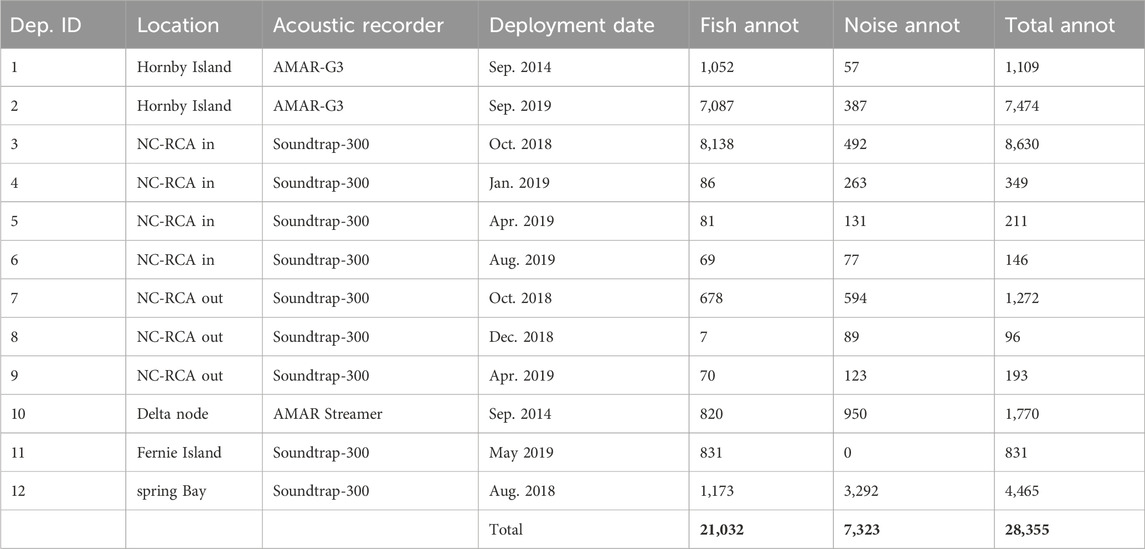
Table 1. Description of Dataset 1 collected in the Strait of Georgia, British Columbia Canada.

Figure 1

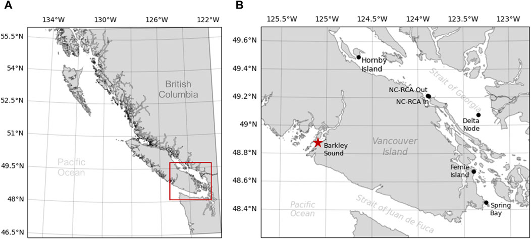
Figure 1. Map of the sampling locations for Dataset 1 (black dots) and Dataset 2 (red star) collected in British Columbia, Canada. The red rectangle in (A) indicates the zoomed-in area represented in (B). NC-RCA In and NC-RCA Out indicate recorders deployed inside and outside the Northumberland Channel Rockfish Conservation Area, respectively.

Data were manually annotated by seven analysts. The annotation protocol differed slightly depending on the deployment, but in all cases, the analysts annotated individual fish sounds rather than grouping several sounds into a single annotation. Other sounds were also annotated and included marine mammal calls (e.g., killer whale, harbor seal), anthropogenic and environmental sounds (e.g., vessels, waves), and pseudo noise (e.g., flow noise, objects touching hydrophone). Noise annotations were also performed semi-automatically. First, sections of audio recordings not containing any fish sounds were identified by analysts. Then, a detector (Section 2.3.1) was run on the selected recordings to automatically define the time and frequency boundaries of all acoustic transients. Recordings used to create this noise dataset were chosen so it would include a large variety of sounds such as noise from vessels, moorings, surface waves, and invertebrates.

All fish annotations are labelled as such (“fish”), while all non-fish annotations are grouped into the label “noise” (Table 1). The entire dataset includes 21,032 fish annotations and 7,323 noise annotations, is composed of 670 audio files (each being either 5-min or 30-min long depending on the deployments) and represents a total of 133.75 h of accumulated acoustic recordings.

2.1.2 Dataset 2: Barkley sound, Canada

Data from the second dataset were collected in Barkley Sound, on the West coast of Vancouver Island, British Columbia, Canada using an M36 hydrophone (Geospectrum Technologies Inc.) connected to an AMAR recorder (JASCO Applied Sciences) deployed on the seafloor (water depth: 21 m) from 9 September 2022 to 16 September 2022. The recorder acquired data continuously with a sampling frequency of 32 kHz. Two analysts fully annotated four 30-min files per day by selecting each file randomly within each 6-h period of the day. Thirty files were fully annotated, representing an accumulated recording duration of 15 h spread out over a period of 7 days. The dataset contains a total of 5,431 annotated fish sounds (Table 2).

Table 2

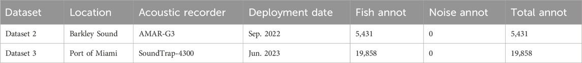
Table 2. Description of datasets 2 and 3.

2.1.3 Dataset 3: Port of Miami, United States

Data from the third dataset were collected in the Port of Miami, FL, Unitesd States from 7 June 2023 to 15 June 2023, as part of the 2023 World Oceans Passive Acoustic Monitoring (WOPAM) Day (Figure 2). Data were collected using a HTI-96-Min hydrophone (High Tech Inc.) connected to a SoundTrap 4,300 recorder (Ocean Instruments) and placed on the seafloor (water depth: 3 m) near the Coral City Camera (Coral Mophologic: www.coralcitycamera.com). The recorder acquired data continuously at a sampling frequency of 144 kHz. An analyst annotated all fish sounds in the first 5 minutes of each hour for each day of the deployment. One hundred and ninety (190) files were fully annotated which represents an accumulated recording duration of 15.8 h spread out over 8 days. The analyst annotated a total of 19,858 fish sounds (Table 2).

Figure 2

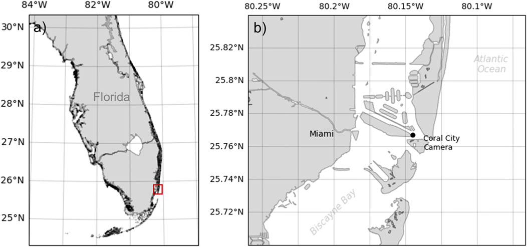
Figure 2. Map of the sampling location for Dataset 3 collected in the port of Miami, Florida, United States. The red rectangle in panel (A) indicates the zoomed-in area represented in panel (B). The acoustic recorder was located near the Coral City Camera.

2.2 Spectrogram calculation and denoising

For all detection approaches, spectrogram calculation and denoising (equalization) is the first processing step. The spectrograms were calculated using 0.064 s long frames, 0.064 s long FFTs (i.e., no zero-padding), and time steps of 0.01 s. This resolution was selected as it can represent well the different types of fish sounds (i.e., grunts and knocks). Given that all fish sounds of interest in this study have frequencies below 1.2 kHz, the spectrogram is truncated to only keep frequencies from 0 to 1.2 kHz. Magnitude values are squared to obtain energy and expressed in decibels. To improve the signal-to-noise ratio of fish sounds and attenuate tonal sounds from vessels, the spectrogram is equalized using a median filter, calculated with a sliding window, for each row (frequency) of the spectrogram. The equalized spectrogram, $\widehat{S}[t,f]$, at each time bin, $t$, and frequency bin, $f$, is calculated as:

$\widehat{S}\left[t,f\right]=S\left[t,f\right]-S_{\mathit{med}}\left[t,f\right],(1)$

where $S[t,f]$ is the original spectrogram and $S_{\mathit{med}}[t,f]$ is the median spectrogram calculated as:

$S_{\mathit{med}}\left[t,f\right]=\mathrm{m}\mathrm{e}\mathrm{d}\mathrm{i}\mathrm{a}\mathrm{n}\left(S\left[t-k,f\right],S\left[t-k+1,f\right],\dots ,S\left[t,f\right],\dots ,S\left[t+k-1,f\right],S\left[t+k,f\right]\right),(2)$

where the median is calculated on a window centered on the $t^{th}$ sample and has a duration of $2k+1$ bins. Figure 3A shows the equalized spectrogram. Here, we choose a median window equivalent to a 3 s duration $(k=150)$, which removes constant tonal components from vessels without removing the longer grunting sounds from fish.

Figure 3

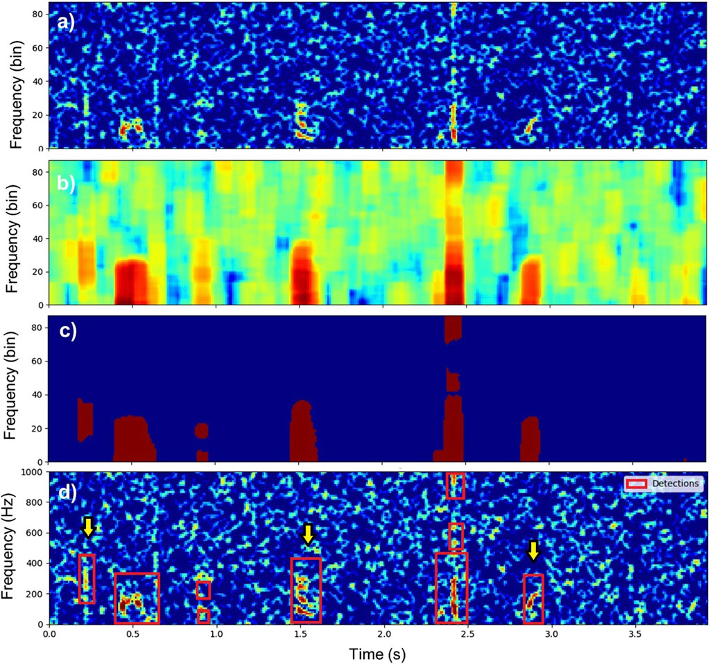
Figure 3. Illustration of the detection process on a recording containing three fish sounds. (A) Equalized spectrogram $\widehat{S}[t,f]$, (B) local variance matrix $S_{\mathit{var}}[t,f]$, (C) binarized spectrogram, (D) result of the detection process. Red boxes indicate the time and frequency boundaries of each detected event. Fish sounds are at $t=0.2$ s, $t=1.5$ s, and $t=2.8$ s (yellow arrows).

2.3 Approach 1: Random forest

The first approach implemented to detect fish sounds is based on the RF classification algorithm. It consists of 1) segmenting the spectrogram to detect acoustic transients, 2) extracting features for each detected event, and 3) classifying each event using a binary (“fish” vs. “noise”) RF classifier.

2.3.1 Spectrogram segmentation

Once the spectrogram is calculated and equalized, it is segmented by calculating the local energy variance on a two-dimensional (2D) kernel of size $\mathrm{\Delta }T\times \mathrm{\Delta }F$. The resulting matrix $S_{\mathit{var}}$ (Figure 3B) is defined as

$S_{\mathit{var}}\left[t,f\right]=\frac{1}{\left(\mathrm{\Delta }T\mathrm{\Delta }F\right)-1}{\displaystyle \sum _{i=t-\frac{\mathrm{\Delta }T}{2}}^{t+\frac{\mathrm{\Delta }T}{2}}}{\displaystyle \sum _{j=f-\frac{\mathrm{\Delta }F}{2}}^{f+\frac{\mathrm{\Delta }F}{2}}}|\widehat{S}\left[i,j\right]-\mu {|}^2,(3)$

where $\mu$ is the mean over the 2D kernel:

$\mu =\frac{1}{\left(\mathrm{\Delta }T\mathrm{\Delta }F\right)}{\displaystyle \sum _{i=t-\frac{\mathrm{\Delta }T}{2}}^{t+\frac{\mathrm{\Delta }T}{2}}}{\displaystyle \sum _{j=f-\frac{\mathrm{\Delta }F}{2}}^{f+\frac{\mathrm{\Delta }F}{2}}}\widehat{S}\left[i,j\right].(4)$

In this study, the number of time and frequency bins of the kernel are chosen to be equivalent to 0.1 s and 300 Hz, respectively. Bins of the spectrogram with a local variance less than 10 are set to zero and all the other bins are set to one (Figure 3C). Bounding boxes of contiguous bins in the binarized spectrogram are then defined using the outer border following algorithms described in Suzuki and Be (1985). These bounding boxes define acoustic events of interest (red rectangles in Figure 3D) and are used in the next steps to determine whether they are fish sounds or not. To speed up the classification process, all detected acoustic events shorter than 50 ms or with a bandwidth smaller than 40 Hz are discarded. Figure 3 illustrates the detection process on an acoustic recording containing three fish sounds.

2.3.2 Feature extraction

Each detection is represented by 45 features calculated from the (equalized) spectrogram, the spectral envelope, and the temporal envelope of the detected events (Figure 4; Table 3). The spectral envelope is the sum of the spectrogram energy values for each frequency (Figure 4B). The temporal envelope is the sum of the spectrogram energy values for each time step (Figure 4C). The spectral and temporal envelopes are normalized to 1 and interpolated to have a resolution of 0.1 Hz and 1 ms, respectively (red dots in Figures 4B, C). Spectrogram features are extracted based on a time-frequency box that contains $95\%$ of the energy of the initial detection (white box in Figure 4A). Table 3 describes all features calculated to represent the detections. Features are normalized before being used for classification, so all have a mean of 0 and a variance of 1. These features were selected as they were shown to successfully represent animal sounds in a number of studies (e.g., Acevedo et al., 2009; Ross and Allen, 2014; Mouy et al., 2013).

Figure 4

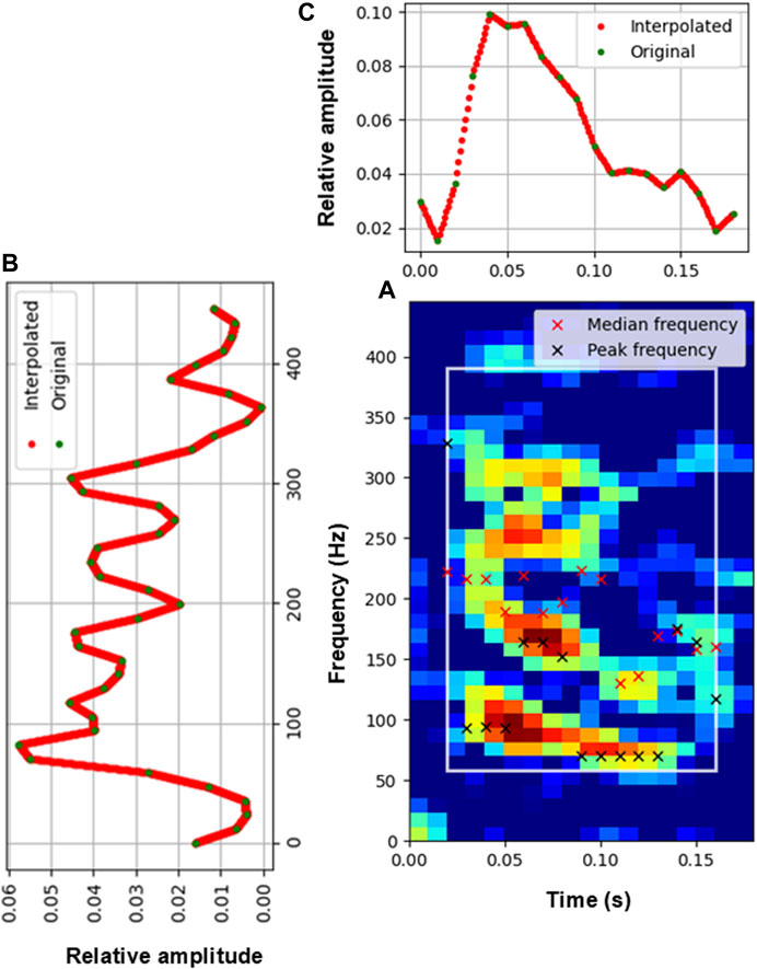
Figure 4. Extraction of features. (A) Spectrogram of a fish detection. Red and black crosses denote the median and peak frequency of each time slice of the spectrogram, respectively. The white box indicates the $95\%$ energy area over which the spectrogram features were calculated. (B) Spectral envelope of the detection. (C) Temporal envelope of the detection.

Table 3

Table 3. Description of the features calculated for each detection.

2.3.3 Random forest classification

Features described in Section 2.3.2 are used to classify the detected events as either “fish” or “noise.” Random forest is a classification technique based on the concept of an ensemble. A RF is a collection of decision trees (Breiman, 2001), where each tree is grown independently using binary partitioning of the data based on the value of one feature at each split (or node). When features measured from a sample or, in our case, a sound, are run through the RF, each tree in the forest produces a classification and the sound is classified as the class that the greatest number of trees vote for. Randomness is injected into the tree-growing process in two ways: 1) each tree in the forest is grown using a random subsample of the data in the training dataset and 2) the decision of which feature to use as a splitter at each node is based on a random subsample of all features (Breiman, 2001). Each tree is grown to its maximum size. Using an ensemble of trees with splitting features chosen from a subset of features at each node means that all important features will eventually be used in the model. In contrast, a single decision tree is limited to a subset of features (unless the number of features is small or the tree is large) and can be unstable (small changes in the dataset can result in large changes in the model; Breiman, 1996). The ensemble decision approach typically results in lower error rates than can be achieved using single decision trees (e.g., Bauer and Kohavi, 1999). In this study, we tested RF models with 5, 10, and 50 trees (noted as RF5, RF10, and RF50, respectively). For all these test models, the random subset of features used for each splits was set to 6.

2.4 Approach 2: Convolutional neural network

The second detection approach implemented is based on Convolutional Neural Networks (CNN, Goodfellow et al., 2016). Like the first approach, it relies on the spectrogram representation of the acoustic signal (Section 2.2). However, contrary to more traditional machine learning approaches like RF, the features are not “hand crafted” by a domain expert (as done in Section 2.3.2) but are directly learned from the data. CNN typically comprise a sequence of convolutional layers followed by a few fully connected layers. Convolutional layers are responsible for detecting features in the input data by applying convolution operations with learnable filters. These layers capture spatial hierarchies of features, starting from simple patterns like edges and textures and progressing to more complex and abstract representations. Fully connected layers are placed at the end of the network and are responsible for making final classifications based on the features learned in earlier layers (Goodfellow et al., 2016). Here, we use a residual network (ResNet) with the same architechture as Kirsebom et al. (2020). It uses residual blocks that contain shortcut connections that allow the network to learn residual functions, which are the differences between the desired mapping (the output of a layer) and the input to that layer (He et al., 2016). By learning these residuals, the network can effectively train very deep architectures without encountering the vanishing gradient problem. We used residual blocks with batch normalization (Ioffe and Szegedy, 2015) and rectified linear units (ReLU, Nair and Hinton, 2010). The number of filters for the initial convolutional layer was set to 16 and was doubled for each subsequent block. The final network was composed of one initial convolutional layer, followed by eight residual blocks, a batch normalization layer, a global average pooling layer (Lin et al., 2013), and a fully connected layer with a softmax function for classification. While we used the same network architecture as Kirsebom et al. (2020), we retrained the entire model (i.e., all layers, no transfer learning) using the training dataset.

The ResNet is run on overlapping slices of spectrogram and provides a classification score betweeen 0 and 1 to indicate the probability that the slice analyzed contains a fish sound. To distinguish individual fish sounds, the classification is performed for every 0.01 s of recording on 0.2 s-long spectrogram slices (with a frequency band of 0–1.2 kHz). Spectrogram slices with a classification score exceeding the user-defined threshold are considered fish sound detections. Consecutive detections are merged into a single detection and its final classification score is the maximum score of the merged detections. To ensure that the spectrogram slices presented to the CNN always have the same size ($20\times 78$ bins), all recordings analyzed are first downsampled to 4 kHz (i.e., bandwidth of 2 kHz).

Training was conducted using a NVidia A100SXM4 (40 GB memory) graphical processing unit (GPU) and was performed with a batch size of 32 over 50 epochs. Network weights were optimized to maximize the $F_1$ score using the ADAM optimizer (Kingma and Ba, 2014) set with its default parameters (learning rate = 0.001, decay = 0.01, b1 = 0.9, b2 = 0.999). To increase the quantity and variability of the training samples, time-shift augmentation was used. This consisted of creating multiple instances of the same selection by stepping in time, both forward and backward from the middle point of the original annotation. Augmented samples were created by shifting 0.2 s long windows by 0.1 s increments and by ensuring that each of the created samples overlapped in time by at least 90$\%$ with the original annotation.

2.5 Experimental design

Random forest and CNN models were trained and tested by dividing annotated sounds of Dataset 1 (Section 2.1.1) into two subsets. One was composed of 75% of the entire dataset and was used to train the classification models, tune their hyperparameters, and identify which one performed best. The other one, representing 25% of Dataset 1, was used to evaluate the performance of the selected model. These two subsets were carefully defined so annotations from each subset were separated by at least 6 hours, had the two classes (fish and noise) equally represented, and had a similar representation of all deployments. Data used for testing the performance of the classification were not used for training the models. In addition to being tested on part of Dataset 1, the detectors were tested on Datasets 2 and 3. Testing performance on Dataset 2 provides information on how well detectors perform on sounds from similar fish species, but in a different environment. Testing performance on Dataset 3 provides information on how versatile the detectors are to new environments and quantifies their ability to detect sounds from fish species they were not trained on.

2.6 Performance

The decisions generated from the detectors can be categorized as follows.

$•$ True positives $(TP)$: A fish sound correctly classified as a fish sound;

$•$ False positives $(FP)$: Noise classified as a fish sound (i.e., a false alarm); and

$•$ False negatives $(FN)$: A fish sound classified as noise (i.e., missed).

To calculate the numbers of $TP$s, $FP$s, and $FN$s, the manual annotations of fish sounds, which are considered true results, are compared with the automated detections. To assess the performance of the detectors, precision $(P)$ and recall $(R)$ metrics are calculated based on the numbers $(N)$ of $TP$s, $FP$s, and $FN$s, as:

$P=\frac{N_{TP}}{N_{TP}+N_{FP}},R=\frac{N_{TP}}{N_{TP}+N_{FN}},(5)$

where $P$ measures exactness and $R$ measures completeness. For instance, a $P$ of 0.9 means that 90% of the detections classified as fish sounds are in fact fish sounds but says nothing about whether all sounds in the dataset are identified. An $R$ of 0.8 means that 80% of all fish sounds in the dataset are correctly classified, but says nothing about how many classifications are wrong. Thus, a perfect classifier would have $P$ and $R$ equal to 1. Neither $P$ nor $R$ alone can describe the performance of a detector/classifier on a given dataset; both metrics are required. The $F$ score is also used to quantify classifier performance. The $F$ score measures the accuracy of the detector and varies from 0 to 1, where an $F$ score of 1 corresponds to a perfect detector. It is defined as

$F_{\beta }=\left(1+{\beta }^2\right)\frac{PR}{{\beta }^{2}P+R},(6)$

where $\beta$ is the relative weight between the recall and precision. A $\beta$ of two means the recall has twice the weight of the precision. Conversely, a $\beta$ of 0.5 means the recall has half the weight of the precision. In this work, it is considered that $P$ and $R$ are equally important, so the unweighted $F_1$ score is used (i.e., $\beta =1$). Note that we did not assess the performance for each sound type separately (i.e., pulse, grunts, tones) as the annotation datasets were not labelled to the sound type level.

All classifiers used in this study provide binary classification results (i.e., “fish” or “noise”) as well as a confidence of classification between 0 and 1. The latter can be used to adjust the sensitivity of a classifier. Accepting classification results with a low confidence leads to detecting more fish sounds (high recall), but also generates more false alarms (low precision). Conversely, only accepting classification results with a high confidence leads to detecting fewer fish sounds (low recall), but also results in fewer false alarms (high precision). The optimum confidence threshold is considered as the one providing the highest $F$ score. It is defined experimentally by iteratively calculating the performance for small increments (here 0.001) of confidence threshold values from 0 to 1.

2.7 Signal to noise ratio

Detector performance is characterized for different signal-to-noise ratios (SNR). The SNR of an annotated fish sound is defined as the ratio of the signal power $(P_s)$ to the noise power corrupting the signal $(P_n)$. The SNR compares the level of the desired signal (i.e., a fish sound) to the level of the background noise. The greater the SNR, the less obtrusive the background noise is. The SNR is defined in decibels as:

$SNR=10{\log }_{10}\left(P_s/P_n\right).(7)$

For this study, $P_s$ is the average power of the fish sound over the duration in seconds, $d$, of the sound in the frequency band defined by the analyst (i.e., frequency boundaries of the annotation box); $P_n$ is the average of the power within the same frequency band $d/2$ seconds before and after the fish sound. Both $P_s$ and $P_n$ are calculated from the waveform filtered in the frequency band defined by the analyst who generated the annotations (10th order Butterworth bandpass filter).

2.8 Sound pressure levels

Sound pressure levels (SPL) were calculated on data from Dataset 2 and Dataset 3 to investigate relationships between noise levels and detector performance (section 3.4). An end-to-end calibration was performed for each hydrophone using a piston-phone type 42AA precision sound source (G.R.A.S. Sound $\&$ Vibration A/S) at 250 Hz. System gains for Dataset 2 (AMAR recorder) and Dataset 3 (SoundTrap recorder) were $-167.3$ dB re FS/$\mu$Pa and $-168.2$ dB re FS/$\mu$Pa, respectively. SPLs were calculated between 20 and 1,000 Hz (i.e., the frequency band of most fish sounds) for each minute of recording using the software PAMGuide (Merchant et al., 2015) in Matlab (MathWorks Inc.).

2.9 Implementation

All algorithms described in this work are implemented in Python. Spectrogram calculation and denoising (section 2.2) are conducted using the libraries NumPy (Harris et al., 2020), Dask (Dask Development Team, 2016) and ecosound (Mouy, 2021). The RF classification (section 2.3) is implemented using the scikits-learn library (Pedregosa et al., 2011). The CNN (section 2.4) was trained using the library Ketos (Kirsebom et al., 2021). Along with this paper, we provide the open source (BSD-3-Clause License) software FishSound Finder (https://github.com/xaviermouy/FishSound_Finder) allowing others to easily run the CNN detector on acoustic recordings and output detection results as NetCDF files and Raven tables. FishSound Finder is documented and includes tutorials for users not familiar with the python language.

3 Results

This section summarizes the performance results of the RF and the CNN on the three different datasets.

3.1 Dataset 1: Strait of Georgia, Canada

Figure 5 shows the precision-recall curve for RF (blue) and CNN (black). Three RF models were trained using 5, 10 and 50 trees. The increase in the number of trees in the RF model from 5 to 50 raises the maximum $F_1$ score by 0.02 ($F_1$ = 0.68 for RF5 and $F_1$ = 0.70 for RF50). The model with 50 trees performs the best of all RF models with a recall $R=0.72$ and a precision $P=0.67$. Maximum performance for all RF models is achieved with a detection threshold of 0.6.The CNN models were always trained using the maximum number of (augmented) fish sound examples available in the training dataset (i.e., 20,000), but the number of noise examples used for training was varied in order to investigate how imbalanced datasets impact the performance of the CNN. Three CNN models were trained: one using 20,000 noise examples (i.e., balanced dataset, dotted black line, Figure 5), one with 40,000 noise examples (dashed black line in Figure 5), and one with the entire set of noise examples available in the training set (i.e., 198,461 noise examples, solid black line in Figure 5). Note that the number of training examples indicated here is larger than the number of annotations in Table 1 because of the time-shift data augmentation process explained in Section 2.4. Increasing the number of noise examples from 20,000 to 40,000 raises the maximum $F_1$ score by 0.03 (from 0.82 to 0.85) but has no noticeable effect when increasing from 40,000 to 198,461 noise examples. The best CNN performance is achieved by the model trained with the entire noise dataset. The best $F_1$ score for that model is reached with a detection threshold of 0.99 and has a precision of $P=0.85$ and a recall of $R=0.84$. Overall, based on the $F_1$ score, the best CNN model performs 1.2 times better than the best RF model.

Figure 5

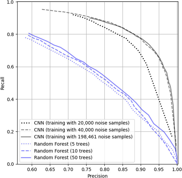
Figure 5. Performance of the RF (blue lines) and CNN (black lines) on the Strait of Georgia dataset (Dataset 1). Dotted, dashed and full blue lines represent the performance of the RF with 5, 10 and 50 trees, respectively. Dotted, dashed and full black lines represent the performance of the CNN trained with 20,000, 40,000, and 198,461 noise samples, respectively.

Most of the annotated fish sounds in the test dataset have a low SNR (Figures 6A, C, D). In order to have a more complete understanding of the performance, Figure 6B shows a break down of the performance of the best CNN for very faint (SNR$<$3.4 dB, Figure 6C), faint (3.4 dB$\le$ SNR$<$6.3 dB, Figure 6D) and loud (SNR$\ge$6.3 dB, Figure 6D) fish sounds. Limits for each SNR category were defined such that there is an equal number of fish sounds in each SNR interval (Figure 6A). At maximum $F_1$ scores, the CNN can detect very faint fish sounds with a precision of $P=0.74$ and a recall of $R=0.72$; faint fish sounds with a precision of $P=0.77$ and a recall of $R=0.72$; and loud fish sounds with a precision of $P=0.82$ and a recall of $R=0.83$.

Figure 6

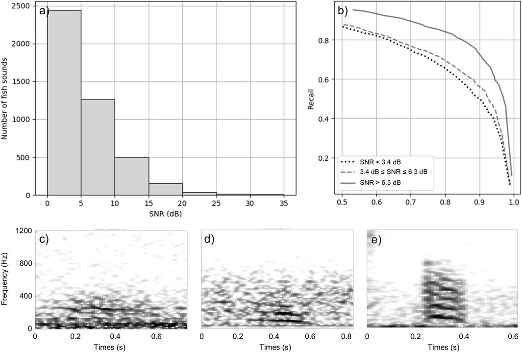
Figure 6. Performance of the best CNN by SNR interval. (A) Distribution of the SNR of fish sounds in the test dataset. (B) Precision-recall curve for very faint (SNR$<$3.4 dB), faint (3.4 dB$\le$SNR$\le$ 6.3 dB) and loud (SNR$>$6.3 dB) fish sounds. (C–E) show example spectrograms of very faint, faint, and loud fish sounds, respectively.

3.2 Dataset 2: Barkley Sound, Canada

Performance of the CNN on the Barkley Sound dataset was initially evaluated using the manual annotations performed by the analyst. The performance obtained, depicted by the dashed line in Figure 7A, was lower than expected considering the results from Dataset 1 (Figure 5). From these results, it appeared that the CNN could detect a large fraction (91 $\%$) of the fish sounds annotated by the analyst $(R=0.91)$, but generated a very large number of false alarms $(P=0.07)$. Upon further investigation of the detection results, it appeared that the CNN detected a large number of faint fish sounds that the analyst did not see/hear (see Figure 7B). All detections from the CNN were therefore reviewed by another analyst to decide if they were fish sounds or false positives (i.e., noise). After this re-annotation process, the dataset went from 1,331 fish annotations to 5,431 (Table 2). Performance of the CNN was re-evaluated using the updated dataset and showed results consistent with what was calculated with Dataset 1. For the detection threshold (0.912) providing the highest $F_1$ score $(F_1=0.82)$, the recall is $R=0.94$ and the precision $P=0.73$. Inspection of the false positives shows that the majority of false alarms occur on only three recordings and are generated by a low-frequency tapping sound from a loose cable hitting the instrument frame during periods of high current (Figure 7).

Figure 7

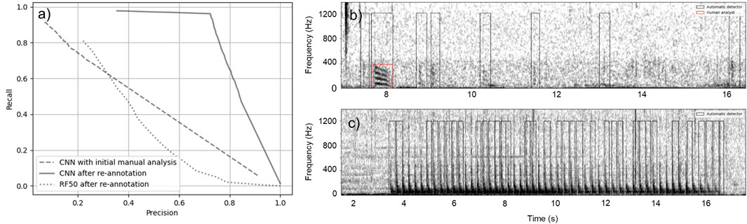
Figure 7. Performance of RF and CNN on Dataset 2. (A) Precision-recall curves for the CNN on the original dataset (dashed line), for the CNN on the re-annotated dataset (solid line), and for RF on the re-annotated dataset (dotted lines). (B) Spectrogram of a recording containing eight fish sounds. The red box indicates the fish sound initially annotated by the analyst and the black boxes show the fish sounds that were detected by CNN, but missed by the analyst. (C) Example of mooring noise triggering most of the false alarms of the CNN.

Performance of the RF on this dataset is substantially lower than on Dataset 1 with a maximum $F_1$ score $F_1=0.43$ ($P$ = 0.38, $R=0.51$, threshold = 0.74, dotted line in Figure 7). The difference in performance between the CNN and RF is more pronounced than for Dataset 1, with a best $F_1$ score for the CNN 1.9 higher than for RF.

3.3 Dataset 3: Port of Miami, United States

Figure 8A shows the performance curve of the CNN on the dataset collected in the Port of Miami. Maximum $F_1$ score $(F_1=0.89)$ is reached with a detection threshold of 0.1 and corresponds to a recall $R=0.86$ and precision $P=0.91$. False alarms are mostly generated by broadband pulses from invertebrates (e.g., snapping shrimp) with a low-frequency component. Fish sounds missed by the CNN are mostly pulse trains occurring at night that have a higher peak frequency ($>$800 Hz) than the typical fish sounds found in Datasets 1 and 2 (e.g., pulse trains in Figure 8C starting at $t=$ 2 s and $t=$ 6.1 s) and fainter pulse trains (e.g., fish sound at $t=$7.9 s in Figure 8B).

Figure 8

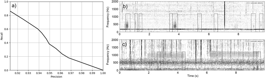
Figure 8. Performance of the CNN on Dataset 3. (A) Precision-recall curve of the CNN on Dataset 3. (B) Example of fish sounds detected by the CNN. This example includes 11 fish sounds: nine are detected by the CNN but 2 fainter fish sounds are missed (at $t=$ 5 s and $t=$ 7.9 s). (C) Example of higher frequency fish pulse trains missed by the CNN ($t=$ 2 s and $t=$ 6.1 s). Black boxes indicate detections from the CNN.

3.4 Influence of noise levels on detector performance

Detectors are not perfect; however, by characterizing their limitations, it is possible to better understand in which conditions their outputs can be trusted and in which conditions they should not be used without manual verification. Figure 9 shows how the number of detections from the CNN aligns with the number of fish sounds manually annotated for different ambient noise conditions. For Barkley Sound, SPLs in the 20–1,000 Hz frequency band ranged from 70 to 130 dB re 1$\mu$Pa. For minutes of recording with a SPL below 100 dB re 1$\mu$Pa, the number of detections from the CNN is strongly correlated ($R^2$ = 0.82) with the number of detections found by the analyst (Figure 9A; Table 2). However, for minutes of recording with a SPL greater than 100 dB re 1$\mu$Pa (Figure 9C), this relationship is highly degraded ($R^2$ = 0.51) and the detector outputs cannot be used without manual verification. Such degradation of the detector performance at these SPL is due to the intense mooring noise reported for this dataset in section 3.2 (Figure 7C).

Figure 9

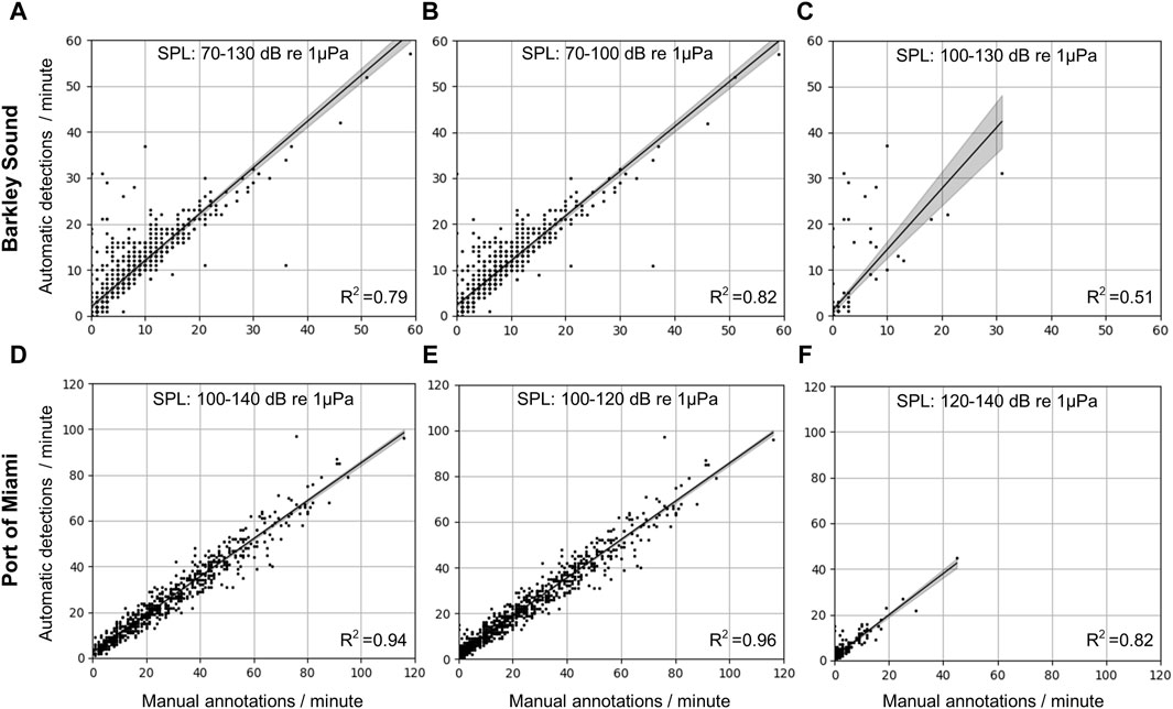
Figure 9. Comparison of the number of fish sounds detected by the CNN and the human analyst in different noise conditions for the Barkley Sound (top row) and the Port of Miami (bottom row) datasets. (A–C) Correlation plots for the Barkley Sound dataset for SPL intervals [70,130] [70,100], and [100,130] dB re 1$\mu$Pa, respectively. (D–F) Correlation plots for the port of Miami dataset for SPL intervals [100,140] [100,120], and [120,140] dB re 1$\mu$Pa, respectively. Solid black lines and shaded grey areas indicate the linear regression lines and the 95$\%$ confidence intervals, respectively. All SPLs are calculated per minute in the 20–1,000 Hz frequency band (Section 3.4).

For the Port of Miami dataset, SPLs in the 20–1,000 Hz frequency band range from 100 to 140 dB re 1$\mu$Pa. Despite higher SPLs than the Barkley Sound dataset, the overall number of fish detections per minute from the CNN correlates well with the number of fish sounds found by the analyst ($R^2=$ 0.94, Figure 9D), even for noise levels greater than 120 dB re 1$\mu$Pa ($R^2=$ 0.82, Figure 9F).

4 Discussion

We implemented and compared two approaches to detect fish sounds. One is based on RF, which is a traditional classification machine learning method that has been successful in previous bioacoustic classification tasks. The other is based on a deep neural network architecture which is a technique that recently outperformed more traditional classification methods (Shiu et al., 2020). Methods like RF require defining a set of features that represent the signal of interest and are used to discriminate between the different sound classes (e.g., fish sounds vs. noise). This set of features is typically defined (“hand crafted”) by domain experts who understand which features are the most discriminative. These features can be hard to define and may be highly dependent on noise conditions. Even with high-performing classifiers, poorly chosen features will result in poor classification performance. Deep neural networks, such as the CNN used in this work, bypass this step and consider the definition of salient signal features as part of the training process. The first convolutional layers of the CNN are responsible for finding the salient features of the signal (filters) that maximize classification success. Both the features definition and the classification are optimized in unison and are learned directly from the data.

We found that CNN performs substantially better than RF on all datasets. Increasing the number of trees in the RF model increased the classification performance but not enough to outperform the CNN. The decrease of 27$\%$ in $F_1$ score between the Strait of Georgia (where the model was trained) and Barkley Sound indicates that the RF model does not generalize well enough and is not adaptable to new acoustic environments. Conversely, the CNN had a satisfactory performance on all datasets. Training the CNN using more noise examples than fish sounds (i.e., imbalanced training dataset) improved the classification performance. Despite being trained on data from the Strait of Georgia, the CNN performed well on the Barkley Sound data. This result indicates that the model generalized well and was reliable in environments with different noise conditions. This is further demonstrated by the consistent performance of the CNN on data from the Port of Miami, which include high noise levels due to intense vessel traffic. While the Strait of Georgia and Barkley Sound share a large number of similar fish species, the Port of Miami has tropical fish species that are very different from the Canadian datasets. The consistent performance of the CNN in the Port of Miami shows that the model not only learned to recognize Canada-specific fish sounds, but also learned general fish sound characteristics which can be applied in different ecosystems.

The Sciaenidae sound detector described in Harakawa et al. (2018) and the generic fish detector in Malfante et al. (2018) (both machine learning-based) achieved a $F_1$ score of 0.86 and 0.9 on their datasets, respectively, which is comparable to the best $F_1$ score we obtained with the CNN ($F_1=$ 0.89). Waddell et al. (2021) also developed a detector to recognize six different types of fish sounds in a long-term passive acoustic monitoring dataset from the northern Gulf of Mexico. The classification was also based on a ResNet CNN architecture but was trained using transfer learning. Its performance ranged from $F_1$ = 0.44 to $F_1$ = 0.77 depending on the sound types targeted. Note that the latter study had a restricted number of manual annotations available to train some of the call types and performed a multi-class classification task which is more complex than the binary classification of our work. Munger et al. (2022) also developed a detector based on a ResNet CNN trained via transfer learning and achieved a $F_1$ score of 0.86. The latter was solely focused on the detection of sounds from damselfishes in the western Pacific. Using a support vector machine (SVM) based algorithm, Noda et al. (2016) obtained an $F_1$ score of 0.98 for classifying sounds from 128 fish species. However, that study was based on a small dataset of sounds recorded in tanks and did not include classification of noise (i.e., non-fish) recordings. Several other fish sound detectors have been developed but many focus on detecting periodic fish chorusing events rather than individual fish sounds (e.g., Lin et al., 2018; Siddagangaiah et al., 2019; Kim et al., 2023). The calculated performance of automatic detectors and classifiers depends strongly on the datasets used to both train and test the algorithms. Evaluating algorithms on small datasets (e.g., several hundred sounds collected over a few days), where noise conditions, fish species present, and recording platforms do not change or are very stable and predictable, can lead to high performance scores, which may not be representative of how these algorithms would behave when applied to large continuous passive acoustic datasets. The large dataset we use in this work is comprised of more than 53,000 fish and noise sounds collected over eight different sites in both Canada and the United States, and spanning all seasons of the year, providing confidence that the detector characterized in this paper would behave similarly in other areas.

The methods developed here target individual fish knocks and grunts below 1,200 Hz which are sound types commonly recorded worldwide. Longer continuous sounds from chorusing fish, such as plainfin midshipman (P. notatus) hums (Halliday et al., 2018), would not be successfully detected with the proposed methods. For detecting fish choruses, approaches such as the Soundscape learning technique described by Kim et al. (2023) are preferable. As found in the analysis of the data from the Port of Miami, fish sounds with a higher peak frequency than fish sounds typically found in British Columbia tend not to be detected by the CNN (e.g., Figure 8C). To address this limitation, it would be possible to retrain the model with these new sound types. Given the current ability of the CNN model to discriminate noise from fish sounds, it is likely sufficient to freeze the convolutional layers and only retrain the last dense classification layers of the network (i.e., transfer learning), which would only require a few new sound examples. While many fish sounds are below 1,200 Hz, some species like Pacific and Atlantic herring (Clupea pallasii and Clupea harengus) produce sounds at higher frequencies (Wilson et al., 2004). The CNN we proposed here is not able to detect these sounds and a different detector would need to be developed. While the RF detector provides bounding boxes with the minimum and maximum frequencies of the detected sounds, the CNN does not. If such information is required by some users, it is possible to apply the spectrogram segmentation technique from section 2.3.1 on the detections from the CNN. Alternatively, other architectures of CNN providing detection bounding boxes such as Yolo (You Only Look Once, Redmon et al., 2016) could be implemented instead of the ResNet.

Many analysts rely on hearing cues to recognize fish sounds in acoustic recordings. Noise in acoustic recordings and the quality of audio playback equipment (e.g., headphones) can hinder the ability of the analysts to hear fish sounds which leads to fish sounds not being manually detected. As shown on Dataset 2 from Barkley Sound (Section 3.2), the CNN in our work can detect more challenging (i.e., faint) fish sounds than the analyst. While this may not be the case for different datasets or analysts, this illustrates how the CNN can be used as a more consistent way to analyze large passive acoustic datasets. Additionally, analysts are prone to fatigue which induces a non consistent bias and variance in the analysis. Detectors have a bias and variance that are more consistent and predictable than human analysts and can therefore be more easily corrected for. In some cases (e.g., analysis of data from a completely new environment), it may be used as part of the manual analysis to guide the analyst. Characterizing the performance and the limits of detectors is key for answering ecological questions. While the CNN is not perfect and can generate false detections, we show that on the Barkley Sound data these false detections mainly occur when noise levels between 20 and 1,000 Hz exceed 100 re 1$\mu$Pa. In the context of an ecological study, an efficient way to process these data would be to calculate noise levels for every minute of data and focus the manual analysis on the part of the data that has SPL greater than 100 re 1$\mu$Pa. Below that noise level, the detector can be trusted and will require less manual verification effort. As shown by the results from the Port of Miami (Figures 9C–F), this “breaking point” is not always the same and needs to be defined for each dataset analyzed.

Processing 8 days of continuous data at the Port of Miami with the CNN took 6.8 h on a Dell laptop equipped with an Intel(R) Core(TM) i7-8650U CPU at 1.90 GHz and 32 GB of RAM (i.e., 28.2 times faster than real-time) and did not require any human supervision. In comparison, it took approximately 50 h for an analyst to manually analyze 8.3$\%$ of the same dataset (Table 2). Visualization of the outputs from the CNN (Figure 10), allows for quick insights on the temporal patterns of fish sounds and reveals a clear diurnal pattern in the occurrence of fish sounds at that location. The explanation of whether this diurnal pattern is due to fish behaviour or an effect of masking from higher vessel traffic during the day (or both) is not part of this study, but this example illustrates how useful the automatic detector can be to quickly explore passive acoustic datasets, formulate hypotheses, and answer practical conservation questions. Automatic detectors still require some level of manual analysis to validate the detection results. However, several manual analysis methodologies (Kowarski et al., 2021) and software solutions (Mouy et al., 2016; Macaulay, 2021) can be employed to make this process more efficient.

Figure 10

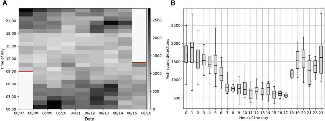
Figure 10. Fish sounds detections at the Port of Miami. (A) Time series of the number of fish sounds detected per hour on the 8 days of continuous data collected at the Port of Miami (June 7–16, 2023). Red horizontal bars indicate the times at which the instrument was deployed and retrieved. (B) Box plot showing the distribution of number of fish sounds for each hour of the day.

Because the CNN detector we provide is not species-specific, it can be used to study and discover general fish occurrence patterns in new environments, help annotate fish sounds in tank or in-situ studies, or be deployed on audio-video systems (e.g., Mouy et al., 2023) to help identify new fish sounds. One reason fish sounds are underused in marine conservation is because the analysis tools developed by engineers and scientists are not always made easily accessible to other researchers in the marine conservation field. Here, we implemented the CNN detector in the easy-to use software FishSound Finder, which is released under an open source license and is accompanied by a step by step tutorial showing how to use it. Our hope is that it will be used, further tested, and improved by other researchers in the community.

Data availability statement

The CNN detector is implemented in the python software FishSound Finder that can be found on GitHub (https://github.com/xaviermouy/FishSound_Finder). The datasets presented in this study can be made available upon request to the corresponding author.

Author contributions

XM: Conceptualization, Data curation, Formal Analysis, Funding acquisition, Investigation, Methodology, Software, Validation, Visualization, Writing–original draft, Writing–review and editing. SA: Data curation, Investigation, Writing–review and editing. SD: Funding acquisition, Resources, Supervision, Writing–review and editing. SD: Funding acquisition, Project administration, Writing–review and editing. PE: Writing–review and editing. CF: Resources, Writing–review and editing. WH: Data curation, Writing–review and editing. FJ: Funding acquisition, Resources, Supervision, Writing–review and editing. DL: Data curation, Writing–review and editing. SV: Funding acquisition, Resources, Writing–review and editing. DH: Funding acquisition, Project administration, Resources, Writing–review and editing.

Funding

The author(s) declare that financial support was received for the research, authorship, and/or publication of this article. This research was funded by Fisheries and Oceans Canada’s (DFO) Competitive Science Research Fund (CSRF) and Strategic Program for Ecosystem-based Research and Advice, Ecosystem Stressors and Aquatic Invasive Species (SPERA), NOAA Fisheries, and the Natural Sciences and Engineering Research Council (NSERC) Canadian Healthy Oceans Network and its Partners: DFO and INREST (representing the Port of Sept-Iles and City of Sept-Iles). Field expenses and equipment costs were funded by a NSERC Discovery grant, the Liber Ero Foundation, CFI/BCKDF, and CSRF Funding. XM was also partly supported by a NSERC Postgraduate Scholarship, JASCO Applied Sciences, and a MITACS Accelerate fellowship.

Acknowledgments

We would like to thank Ocean Networks Canada for providing data from the VENUS cabled observatory (Delta Node) and for providing access to the Advanced Research Computing platform from the Digital Research Alliance of Canada which was instrumental in the training of the deep learning models. Thanks to Jason Gedamke (NOAA Fisheries) for sharing his recorder for the Port of Miami deployment and Katrina Nikolich (University of Victoria) for sharing data from her MSc and PhD. We are grateful to Emie Woodburn, Courtney Evans, Aislyn Adams, Cierra Hart (University of Victoria), and Erik SA (DFO) for manually annotating fish sounds in several of the passive acoustic datasets used in this study. Thanks to David Hannay and Joann Nippard (JASCO Applied Sciences) for their administrative help during this project, Christian Carrera for his help preparing the equipment, and Harald Yurk (DFO) for reviewing an earlier version of this manuscript.

Conflict of interest

The authors declare that the research was conducted in the absence of commercial or financial relationships that could be construed as a potential conflict of interest.

Publisher’s note

All claims expressed in this article are solely those of the authors and do not necessarily represent those of their affiliated organizations, or those of the publisher, the editors and the reviewers. Any product that may be evaluated in this article, or claim that may be made by its manufacturer, is not guaranteed or endorsed by the publisher.

References

Acevedo, M. A., Corrada-Bravo, C. J., Corrada-Bravo, H., Villanueva-Rivera, L. J., and Aide, T. M. (2009). Automated classification of bird and amphibian calls using machine learning: a comparison of methods. Ecol. Inf. 4, 206–214. doi:10.1016/j.ecoinf.2009.06.005

CrossRef Full Text | Google Scholar

Amorim, M. C. P., Stratoudakis, Y., and Hawkins, A. D. (2004). Sound production during competitive feeding in the grey gurnard. J. Fish. Biol. 65, 182–194. doi:10.1111/j.0022-1112.2004.00443.x

CrossRef Full Text | Google Scholar

Amorim, M. C. P., Vasconcelos, R. O., and Fonseca, P. J. (2015). “Fish sounds and mate choice,” in Sound commun. Fishes. Editor F. Ladich (Vienna: Springer Vienna), 1–33. doi:10.1007/978-3-7091-1846-7_1

CrossRef Full Text | Google Scholar

Barroso, V. R., Xavier, F. C., and Ferreira, C. E. L. (2023). Applications of machine learning to identify and characterize the sounds produced by fish. ICES J. Mar. Sci. 80, 1854–1867. doi:10.1093/icesjms/fsad126

CrossRef Full Text | Google Scholar

Bass, A. H., and Ladich, F. (2008). “Vocal–acoustic communication: from neurons to behavior,” in Fish bioacoustics. Editors J. F. Webb, R. R. Fay, and A. N. Popper (New York, NY: Springer New York), 253–278. doi:10.1097/00003446-199510000-00013

CrossRef Full Text | Google Scholar

Bauer, E., and Kohavi, R. (1999). Empirical comparison of voting classification algorithms: bagging, boosting, and variants. Mach. Learn. 36, 105–139. doi:10.1023/a:1007515423169

CrossRef Full Text | Google Scholar

Breiman, L. (1996). Bagging predictors. Mach. Learn. 24, 123–140. doi:10.1007/bf00058655

CrossRef Full Text | Google Scholar

Breiman, L. (2001). Random forests. Mach. Learn. 45, 5–32. doi:10.1023/a:1010933404324

CrossRef Full Text | Google Scholar

Dask Development Team (2016). Dask: library for dynamic task scheduling. Available at: https://dask.org.

Google Scholar

Dubnov, S. (2004). Generalization of spectral flatness measure for non-Gaussian linear processes. IEEE Signal Process. Lett. 11, 698–701. doi:10.1109/LSP.2004.831663

CrossRef Full Text | Google Scholar

Erbe, C., and King, A. R. (2008). Automatic detection of marine mammals using information entropy. J. Acoust. Soc. Am. 124, 2833–2840. doi:10.1121/1.2982368

PubMed Abstract | CrossRef Full Text | Google Scholar

Gannon, D. P., and Gannon, J. G. (2010). Assessing trends in the density of Atlantic croaker (Micropogonias undulatus): a comparison of passive acoustic and trawl methods. Fish. Bull. 108, 106–116.

Google Scholar

Gillespie, D. (2004). Detection and classification of right whale calls using an edge detector operating on a smoothed spectrogram. Can. Acoust. 32, 39–47.

Google Scholar

Goodfellow, I., Bengio, Y., and Courville, A. (2016). Deep learning. MIT press.

Google Scholar

Halliday, W. D., Pine, M. K., Bose, A. P. H., Balshine, S., and Juanes, F. (2018). The plainfin midshipman’s soundscape at two sites around Vancouver Island, British Columbia. Mar. Ecol. Prog. Ser. 603, 189–200. doi:10.3354/meps12730

CrossRef Full Text | Google Scholar

Harakawa, R., Ogawa, T., Haseyama, M., and Akamatsu, T. (2018). Automatic detection of fish sounds based on multi-stage classification including logistic regression via adaptive feature weighting. J. Acoust. Soc. Am. 144, 2709–2718. doi:10.1121/1.5067373

PubMed Abstract | CrossRef Full Text | Google Scholar

Harris, C. R., Millman, K. J., van der Walt, S. J., Gommers, R., Virtanen, P., Cournapeau, D., et al. (2020). Array programming with NumPy. Nature 585, 357–362. doi:10.1038/s41586-020-2649-2

PubMed Abstract | CrossRef Full Text | Google Scholar

He, K., Zhang, X., Ren, S., and Sun, J. (2016). “Deep residual learning for image recognition,” in Proceedings of the IEEE conference on computer vision and pattern recognition, 770–778.

CrossRef Full Text | Google Scholar

Ibrahim, A. K., Chérubin, L. M., Zhuang, H., Schärer Umpierre, M. T., Dalgleish, F., Erdol, N., et al. (2018). An approach for automatic classification of grouper vocalizations with passive acoustic monitoring. J. Acoust. Soc. Am. 143, 666–676. doi:10.1121/1.5022281

PubMed Abstract | CrossRef Full Text | Google Scholar

Ioffe, S., and Szegedy, C. (2015). “Batch normalization: accelerating deep network training by reducing internal covariate shift,” in International conference on machine learning (pmlr), 448–456.

Google Scholar

Kaatz, I. (2002). Multiple sound-producing mechanisms in teleost fishes and hypotheses regarding their behavioural significance. Bioacoustics 12, 230–233. doi:10.1080/09524622.2002.9753705

CrossRef Full Text | Google Scholar

Kim, E. B., Frasier, K. E., McKenna, M. F., Kok, A. C., Peavey Reeves, L. E., Oestreich, W. K., et al. (2023). Soundscape learning: an automatic method for separating fish chorus in marine soundscapes. J. Acoust. Soc. Am. 153, 1710–1722. doi:10.1121/10.0017432

PubMed Abstract | CrossRef Full Text | Google Scholar

Kingma, D. P., and Ba, J. (2014). Adam: a method for stochastic optimization. arXiv preprint arXiv:1412.6980.

Google Scholar

Kirsebom, O. S., Frazao, F., Padovese, B., Sakib, S., and Matwin, S. (2021). Ketos—a deep learning package for creating acoustic detectors and classifiers. J. Acoust. Soc. Am. 150, A164. doi:10.1121/10.0007998

CrossRef Full Text | Google Scholar

Kirsebom, O. S., Frazao, F., Simard, Y., Roy, N., Matwin, S., and Giard, S. (2020). Performance of a deep neural network at detecting North Atlantic right whale upcalls. J. Acoust. Soc. Am. 147, 2636–2646. doi:10.1121/10.0001132

PubMed Abstract | CrossRef Full Text | Google Scholar

Kowarski, K. A., Delarue, J. J.-Y., Gaudet, B. J., and Martin, S. B. (2021). Automatic data selection for validation: a method to determine cetacean occurrence in large acoustic data sets. JASA Express Lett. 1, 051201. doi:10.1121/10.0004851

PubMed Abstract | CrossRef Full Text | Google Scholar

Ladich, F., and Myrberg, A. A. (2006). “Agonistic behaviour and acoustic communication,” in Communication in fishes. Editors F. Ladich, S. P. Collin, and P. Moller (United States: Science Publishers), 122–148.

Google Scholar

Leroy, E. C., Thomisch, K., Royer, J.-Y., Boebel, O., and Van Opzeeland, I. (2018). On the reliability of acoustic annotations and automatic detections of antarctic blue whale calls under different acoustic conditions. J. Acoust. Soc. Am. 144, 740–754. doi:10.1121/1.5049803

PubMed Abstract | CrossRef Full Text | Google Scholar

Lin, M., Chen, Q., and Yan, S. (2013). Network in network. arXiv preprint arXiv:1312.4400.

Google Scholar

Lin, T. H., Fang, S. H., and Tsao, Y. (2017). Improving biodiversity assessment via unsupervised separation of biological sounds from long-duration recordings. Sci. Rep. 7, 1–10. doi:10.1038/s41598-017-04790-7

PubMed Abstract | CrossRef Full Text | Google Scholar

Lin, T.-H., Tsao, Y., and Akamatsu, T. (2018). Comparison of passive acoustic soniferous fish monitoring with supervised and unsupervised approaches. J. Acoust. Soc. Am. 143, EL278–EL284. doi:10.1121/1.5034169

PubMed Abstract | CrossRef Full Text | Google Scholar

Lobel, P. S. (1992). Sounds produced by spawning fishes. Environ. Biol. Fishes 33, 351–358. doi:10.1007/bf00010947

CrossRef Full Text | Google Scholar

Looby, A., Cox, K., Bravo, S., Rountree, R., Juanes, F., Reynolds, L. K., et al. (2022). A quantitative inventory of global soniferous fish diversity. Rev. Fish Biol. Fish. 32, 581–595. doi:10.1007/s11160-022-09702-1

CrossRef Full Text | Google Scholar

Looby, A., Riera, A., Vela, S., Cox, K., Bravo, S., Rountree, R., et al. (2021). FishSounds. Available at: https://fishsounds.net.

Google Scholar

Luczkovich, J. J., Pullinger, R. C., Johnson, S. E., and Sprague, M. W. (2008). Identifying sciaenid critical spawning habitats by the use of passive acoustics. Trans. Am. Fish. Soc. 137, 576–605. doi:10.1577/T05-290.1

CrossRef Full Text | Google Scholar

Macaulay, J. (2021). SoundSort. Available at: https://github.com/macster110/aipam.

Google Scholar

Malfante, M., Mars, J. I., Dalla Mura, M., and Gervaise, C. (2018). Automatic fish sounds classification. J. Acoust. Soc. Am. 139, 2834–2846. doi:10.1121/1.5036628

PubMed Abstract | CrossRef Full Text | Google Scholar

Mann, D. A., Hawkins, A. A. D., and Jech, J. M. (2008). “Active and passive acoustics to locate and study fish,” in Fish bioacoustics. Editors J. F. Webb, R. R. Fay, and A. N. Popper (New York, NY: Springer New York), 279–309. doi:10.1007/978-0-387-73029-5_9

CrossRef Full Text | Google Scholar

Mann, D. A., and Lobel, P. S. (1995). Passive acoustic detection of sounds produced by the damselfish, Dascyllus albisella (Pomacentridae). Bioacoustics 6, 199–213. doi:10.1080/09524622.1995.9753290

CrossRef Full Text | Google Scholar

Mellinger, D. K., and Bradbury, J. W. (2007). Acoustic measurement of marine mammal sounds in noisy environments. Proc. Second Int. Conf. Underw. Acoust. Meas. Technol. Results, Heraklion, Greece, 8.

Google Scholar

Mellinger, D. K., and Clark, C. W. (2000). Recognizing transient low-frequency whale sounds by spectrogram correlation. J. Acoust. Soc. Am. 107, 3518–3529. doi:10.1121/1.429434

PubMed Abstract | CrossRef Full Text | Google Scholar

Merchant, N. D., Fristrup, K. M., Johnson, M. P., Tyack, P. L., Witt, M. J., Blondel, P., et al. (2015). Measuring acoustic habitats. Methods Ecol. Evol. 6, 257–265. doi:10.1111/2041-210X.12330

PubMed Abstract | CrossRef Full Text | Google Scholar

Montie, E. W., Kehrer, C., Yost, J., Brenkert, K., O’Donnell, T., and Denson, M. R. (2016). Long-term monitoring of captive red drum Sciaenops ocellatus reveals that calling incidence and structure correlate with egg deposition. J. Fish. Biol. 88, 1776–1795. doi:10.1111/jfb.12938

PubMed Abstract | CrossRef Full Text | Google Scholar

Moulton, J. M. (1960). Swimming sounds and the schooling of fishes. Biol. Bull. 119, 210–223. doi:10.2307/1538923

CrossRef Full Text | Google Scholar

Mouy, X. (2021). Ecosound bioacoustic toolkit. Available at: https://ecosound.readthedocs.io.

Google Scholar

Mouy, X., Black, M., Cox, K., Qualley, J., Dosso, S., and Juanes, F. (2023). Identification of fish sounds in the wild using a set of portable audio-video arrays. Methods Ecol. Evol. 14, 2165–2186. doi:10.1111/2041-210X.14095

CrossRef Full Text | Google Scholar

Mouy, X., Mouy, P. A., Hannay, D., and Dakin, T. (2016). JMesh-A scalable web-based platform for visualization and mining of passive acoustic data. Proc. - 15th IEEE Int. Conf. Data Min. Work. ICDMW 2015, 773–779doi. doi:10.1109/ICDMW.2015.193

CrossRef Full Text | Google Scholar

Mouy, X., Oswald, J., Leary, D., Delarue, J., Vallarta, J., Rideout, B., et al. (2013). “Passive acoustic monitoring of marine mammals in the Arctic,” in Detect. Classif. Localization mar. Mamm. Using passiv. Acoust. Editors O. Adam, and F. Samaran (Dirac NGO, Paris, France). chap. 9.

Google Scholar

Mouy, X., Rountree, R., Juanes, F., and Dosso, S. (2018). Cataloging fish sounds in the wild using combined acoustic and video recordings. J. Acoust. Soc. Am. 143, EL333–EL339. doi:10.1121/1.5037359

PubMed Abstract | CrossRef Full Text | Google Scholar

Munger, J. E., Herrera, D. P., Haver, S. M., Waterhouse, L., McKenna, M. F., Dziak, R. P., et al. (2022). Machine learning analysis reveals relationship between pomacentrid calls and environmental cues. Mar. Ecol. Prog. Ser. 681, 197–210. doi:10.3354/meps13912

CrossRef Full Text | Google Scholar

Nair, V., and Hinton, G. E. (2010). “Rectified linear units improve restricted Boltzmann machines,” in Proceedings of the 27th international conference on machine learning (Madison, WI, USA: ICML-10), 807–814.

Google Scholar

Nikolich, K., Frouin-Mouy, H., and Acevedo-Gutiérrez, A. (2016). Quantitative classification of harbor seal breeding calls in Georgia Strait, Canada. J. Acoust. Soc. Am. 140, 1300–1308. doi:10.1121/1.4961008

PubMed Abstract | CrossRef Full Text | Google Scholar

Nikolich, K., Halliday, W. D., Pine, M. K., Cox, K., Black, M., Morris, C., et al. (2021). The sources and prevalence of anthropogenic noise in rockfish conservation areas with implications for marine reserve planning. Mar. Pollut. Bull. 164, 112017. doi:10.1016/j.marpolbul.2021.112017

PubMed Abstract | CrossRef Full Text | Google Scholar

Noda, J. J., Travieso, C. M., and Sánchez-Rodríguez, D. (2016). Automatic taxonomic classification of fish based on their acoustic signals. Appl. Sci. 6, 443. doi:10.3390/app6120443

CrossRef Full Text | Google Scholar

Parmentier, E., Lagardère, J. P., Vandewalle, P., and Fine, M. L. (2005). Geographical variation in sound production in the anemonefish Amphiprion akallopisos. Proc. R. Soc. B Biol. Sci. 272, 1697–1703. doi:10.1098/rspb.2005.3146

PubMed Abstract | CrossRef Full Text | Google Scholar

Parsons, M. J., Lin, T.-H., Mooney, T. A., Erbe, C., Juanes, F., Lammers, M., et al. (2022). Sounding the call for a global library of underwater biological sounds. Front. Ecol. Evol. 10, 39. doi:10.3389/fevo.2022.810156

CrossRef Full Text | Google Scholar

Pedregosa, F., Varoquaux, G., Gramfort, A., Michel, V., Thirion, B., Grisel, O., et al. (2011). Scikit-learn: machine learning in Python. J. Mach. Learn. Res. 12, 2825–2830.

Google Scholar

Ramsay, J. O., and Silverman, B. W. (2005). Functional data analysis. 2nd ed. Springer.

Google Scholar

Redmon, J., Divvala, S., Girshick, R., and Farhadi, A. (2016). “You only look once: unified, real-time object detection,” in Proceedings of the IEEE conference on computer vision and pattern recognition, 779–788.

CrossRef Full Text | Google Scholar

Rice, A. N., Farina, S. C., Makowski, A. J., Kaatz, I. M., Lobel, P. S., Bemis, W. E., et al. (2022). Evolutionary patterns in sound production across fishes. Ichthyology & Herpetology 110, 1–12. doi:10.1643/i2020172

CrossRef Full Text | Google Scholar

Riera, A., Rountree, R. A., Agagnier, L., and Juanes, F. (2020). Sablefish (Anoplopoma fimbria) produce high frequency rasp sounds with frequency modulation. J. Acoust. Soc. Am. 147, 2295–2301. doi:10.1121/10.0001071

PubMed Abstract | CrossRef Full Text | Google Scholar

Roch, M. A., Soldevilla, M. S., Burtenshaw, J. C., Henderson, E. E., and Hildebrand, J. A. (2007). Gaussian mixture model classification of odontocetes in the Southern California Bight and the Gulf of California. J. Acoust. Soc. Am. 121, 1737–1748. doi:10.1121/1.2400663

PubMed Abstract | CrossRef Full Text | Google Scholar

Ross, J. C., and Allen, P. E. (2014). Random Forest for improved analysis efficiency in passive acoustic monitoring. Ecol. Inf. 21, 34–39. doi:10.1016/j.ecoinf.2013.12.002

CrossRef Full Text | Google Scholar

Rountree, R. A., Gilmore, G., Goudey, C. A., Hawkins, A. D., Luczkovich, J. J., and Mann, D. A. (2006). Listening to Fish: applications of passive acoustics to fisheries science. Fisheries 31, 433–446. doi:10.1577/1548-8446(2006)31[433:ltf]2.0.co;2

CrossRef Full Text | Google Scholar

Rowell, T. J., Demer, D. A., Aburto-Oropeza, O., Cota-Nieto, J. J., Hyde, J. R., and Erisman, B. E. (2017). Estimating fish abundance at spawning aggregations from courtship sound levels. Sci. Rep. 7, 1–14. doi:10.1038/s41598-017-03383-8

PubMed Abstract | CrossRef Full Text | Google Scholar

Rowell, T. J., Schärer, M. T., Appeldoorn, R. S., Nemeth, M. I., Mann, D. A., and Rivera, J. A. (2012). Sound production as an indicator of red hind density at a spawning aggregation. Mar. Ecol. Prog. Ser. 462, 241–250. doi:10.3354/meps09839

CrossRef Full Text | Google Scholar

Sattar, F., Cullis-Suzuki, S., and Jin, F. (2016). Acoustic analysis of big ocean data to monitor fish sounds. Ecol. Inf. 34, 102–107. doi:10.1016/j.ecoinf.2016.05.002

CrossRef Full Text | Google Scholar

Shiu, Y., Palmer, K. J., Roch, M. A., Fleishman, E., Liu, X., Nosal, E. M., et al. (2020). Deep neural networks for automated detection of marine mammal species. Sci. Rep. 10, 607–612. doi:10.1038/s41598-020-57549-y

PubMed Abstract | CrossRef Full Text | Google Scholar

Siddagangaiah, S., Chen, C. F., Hu, W. C., and Pieretti, N. (2019). A complexity-entropy based approach for the detection of fish choruses. Entropy 21, 1–19. doi:10.3390/e21100977

CrossRef Full Text | Google Scholar

Stolkin, R., Radhakrishnan, S., Sutin, A., and Rountree, R. (2007). “Passive acoustic detection of modulated underwater sounds from biological and anthropogenic sources,” in Ocean. 2007 (vancouver, Canada: ieee), 1–8. doi:10.1109/OCEANS.2007.4449200

CrossRef Full Text | Google Scholar

Suzuki, S., and Be, K. A. (1985). Topological structural analysis of digitized binary images by border following. Comput. Vis. Graph. Image Process. 30, 32–46. doi:10.1016/0734-189X(85)90016-7

CrossRef Full Text | Google Scholar

Tavolga, W. N. (1977). Mechanisms for directional hearing in the sea catfish (Arius felis). J. Exp. Biol. 67, 97–115. doi:10.1242/jeb.67.1.97

PubMed Abstract | CrossRef Full Text | Google Scholar

Thode, A. M., Kim, K. H., Blackwell, S. B., Greene, C. R., Nations, C. S., McDonald, T. L., et al. (2012). Automated detection and localization of bowhead whale sounds in the presence of seismic airgun surveys. J. Acoust. Soc. Am. 131, 3726–3747. doi:10.1121/1.3699247

PubMed Abstract | CrossRef Full Text | Google Scholar

Urazghildiiev, I. R., and Van Parijs, S. M. (2016). Automatic grunt detector and recognizer for Atlantic cod (Gadus morhua). J. Acoust. Soc. Am. 139, 2532–2540. doi:10.1121/1.4948569

PubMed Abstract | CrossRef Full Text | Google Scholar

Waddell, E. E., Rasmussen, J. H., and Širović, A. (2021). Applying artificial intelligence methods to detect and classify fish calls from the northern gulf of Mexico. J. Mar. Sci. Eng. 9, 1128. doi:10.3390/jmse9101128

CrossRef Full Text | Google Scholar

Wilson, B., Batty, R. S., and Dill, L. M. (2004). Pacific and Atlantic herring produce burst pulse sounds. Proc. R. Soc. B Biol. Sci. 271, S95–S97. doi:10.1098/rsbl.2003.0107

PubMed Abstract | CrossRef Full Text | Google Scholar