Combining satellite images with national forest inventory measurements for monitoring postdisturbance forest height growth

Pallissier-Tanon, Agnès; Ciais, Philippe; Schwartz, Martin; Fayad, Ibrahim; Xu, Yidi; Ritter, François; De Truchis, Aurélien; Vega, Cedric; Leban, Jean-Michel

doi:10.3389/frsen.2024.1432577

ORIGINAL RESEARCH article

Front. Remote Sens., 22 August 2024

Sec. Terrestrial Carbon Cycle

Volume 5 - 2024 | https://doi.org/10.3389/frsen.2024.1432577

Combining satellite images with national forest inventory measurements for monitoring post-disturbance forest height growth

Agnès Pellissier-Tanon¹*

Philippe Ciais¹

Martin Schwartz¹

Ibrahim Fayad^1,2

Yidi Xu¹

François Ritter¹

Aurélien de Truchis²

Jean-Michel Leban³

¹Laboratoire des Sciences du Climat et de l’Environnement, LSCE/IPSL, CEA-CNRS-UVSQ, Université Paris Saclay, Gif-sur-Yvette, France
²Kayrros SAS, Paris, France
³Institut National de la Recheche Agronomique—Unité biogéochimie des systèmes forestiers, Nancy, France

Introduction: The knowledge about forest growth, influenced by factors such as tree species, tree age, and environmental conditions, is a key for future forest preservation. Height and age data can be combined to describe forest growth and used to infer known environmental effects.

Methods: In this study, we built 14 height growth curves for stands composed of monospecific or mixed species using ground measurements and satellite data. We built a random forest height model from tree species, age, area of disturbance, and 125 environmental parameters (climate, altitude, soil composition, geology, stand ownership, and proximity to road and urban areas). Using feature elimination and SHapley Additive exPlanations (SHAP) analysis, we identified six key features explaining the forest growth and investigated how they affect the height.

Results: The agreement between satellite and ground data justifies their simultaneous exploitation. Age and tree species are the main predictors of tree height (49% and 10%, respectively). The disturbed patch area, revealing the regeneration method, impacts post-disturbance growth at 19%. The soil pH, altitude, and climatic water budget in summer impact tree height differently depending on the age and tree species.

Discussion: Methods integrating satellite and field data show promise for analyzing future forest evolution.

1 Introduction

Forests are critical to both the environment and human wellbeing and provide services ranging from carbon sequestration to biodiversity conservation and climate regulation (IPCC, 2019). Forest productivity is a major factor of forest resources and, thus, a concern for both forestry and climate sciences. In addition, preserving carbon stocks and maintaining a carbon sink in the forest sector are fundamental elements of the EU Forestry Strategy 2020 and the EU neutrality objectives (Korosuo et al., 2023). In the EU, most forests are managed (FOREST EUROPE, 2020), and management options include rotation ages, thinning regime, regeneration cuttings, the choice of tree species in regeneration and plantation, and forest growth rates (Pretzsch, 2009; Bontemps and Bouriaud, 2014). Natural disturbances can also lead to stand suppression in the case of severe events. The growth rate of forest stands after a management or natural disturbance is linked to the time since the disturbance or stand age, tree species, and site quality (Franklin et al., 2002; Swamy et al., 2003; D’Amato et al., 2011; Luyssaert et al., 2008; Niinemets, 2010; Chazdon et al., 2016; Poorter et al., 2016; Liang et al., 2016; Messier et al., 2019; Pugh et al., 2019; Seidl et al., 2017; Thom et al., 2017). Site quality refers to the intrinsic capacity of local conditions to facilitate the growth of vegetation, and it is influenced by factors such as climate, soil characteristics, topography, and hydrology. Stands located in areas with better site quality have higher growth rates and reach higher carbon stocks at maturity (Swamy et al., 2003; Pan et al., 2011). The importance of forest growth rates has been highlighted in the “Forest Principles” for sustainable forest management at the Rio Conference (UN Conference on Environment and Development, 1992) and confirmed in the criteria for forest management under the Montreal Process (Montreal Process Working Group, 1994) and at the Ministerial Conference on the Protection of Forests in Europe (MCPFE, 2002).

Despite being crucial, determining the growth rates of forests has consistently posed a significant challenge in the field of forestry due to the long-living nature of forest stands and the diversity of development patterns. Several studies analyzed tree height as a function of site-related environmental variables used as proxies of productivity (Bontemps and Bouriaud, 2014; Huang et al., 2017; Günlü et al., 2019; Pretzsch, 2020; Vacek et al., 2023; Viet et al., 2023). Although environmental factors affecting tree growth have been known for decades, these findings are based on a limited amount of field data collected under controlled conditions (Watt et al., 2015; Zhang et al., 2019; Barrio-Anta et al., 2020; Harvey et al., 2020). To remove these limitations, remote sensing data offer sufficient information to conduct an analysis on a large scale and under actual conditions of tree growth (Coops, 2015; Gopalakrishnan et al., 2019; Wang et al., 2022; Antón-Fernández et al., 2023; Appiah Mensah et al., 2023). Remote sensing data may contain significant systematic errors (Palahí et al., 2021; Wernick et al., 2021; Breidenbach et al., 2022). In this context, combining both field and remote sensing data on the same level enhances the accuracy of the resulting products, and some national forest inventories and studies have started to combine both data sources (Tomppo et al., 2008; Nagel et al., 2014; Venier et al., 2014; Breidenbach et al., 2020; Gustafsson et al., 2020; Lister et al., 2020; Næsset et al., 2020; Breidenbach et al., 2021; Schumacher et al., 2020; Sims, 2022).

This study presents one of the first analyses of temperate forest growth detailing tree species, previous disturbance patch areas, and a large number of environmental variables and management practices on a large scale. Our method integrates remote sensing data with inventory measurements to capitalize on the advantages of both data types: the abundance of remote sensing data and the extensive range of tree ages accessible through the inventory data. Thanks to global tree height maps (Besnard et al., 2021; Potapov et al., 2021; Lang et al., 2023), our growth monitoring analysis is applicable to any region across the globe. In this study, our primary objective is to examine the correlation between forest height growth, forest age, species, past disturbance patch size, and a combination of environmental factors to address the following key research questions: (A) can height, age, and tree species data obtained through remote sensing be effectively integrated with similar field measurements? (B) Can we categorize forest growth based on species, and what are the growth disparities between mixed-species forests and pure-species forests? (C) What is the influence of environmental factors beyond age and species on tree height? The study area is a large temperate forest region in the northern-central part of France that has a diversity of tree species and well-documented environmental variables.

We provide an overview of the data sources and processing methods in Section 2. In Section 3, we present a consistency assessment of the two data sources (question A), show the polymorphic age–height curves per species from satellite and field data (question B), and analyze the factors influencing spatial variations in height using explainable machine learning (question C). Then, Section 4 contains a discussion of the results, including the limitations and perspectives.

2 Rationale, datasets, and methods

2.1 Logics of the study

We combined satellite observations and national forest inventory measurements. The methodology consisted of three sequential steps (Figure 1). In the first step (see Figure 1A), we ensured the coherence of the data. This involved assessing the spatial consistency of satellite-derived parameters, tree height, tree age, and tree species, with the corresponding values acquired through field measurements at specific locations. In the second step (see Figure 1B), we modeled the relationship between tree height and age at the species level. To do so, we retrieved tree height, age, and tree species information from satellite observations and the French National Forest Inventory (NFI). These datasets were then integrated to construct empirical growth height–age curves of various tree species, with both satellite and field data. The height–age data were fitted using a Chapman–Richards equation. Additionally, we calculated simple metrics for comparing the height–age curve characteristics of different tree species. In this step, height is explained by age and species only. In the third step (see Figure 1C), we extended our analysis by considering a range of environmental variables, in addition to age and species, to better explain the variations in the height growth. This was done by building an explainable machine learning model to predict the height using the age, species, and the environmental variables as predictive features. This model is made parsimonious using recursive feature elimination to retain only the most influential environmental factors explaining the height. Finally, SHapley Additive exPlanations (SHAP) indexes (Lundberg and Lee, 2017; Lundberg et al., 2020) were used to elucidate the impact of the selected environmental variables on the prediction of tree height.

Figure 1

Figure 1. Flowchart. Input data (in black) are made consistent in step (A) and collocated with ground measurements, allowing us in step (B) to build an empirical height–age relationship for each species. In step (C), an explainable machine learning model is used to predict height from age, species, and environmental factors and separate the influence of each factor.

2.2 Study area

In 2009, the French metropolitan territory was divided into distinct forest regions for taking into account biogeographical factors determining forest production and the distribution of major forest habitat types. In this paper, we study the large ecological region (GRECO) B, which is in north-central France. The GRECO B (north-central semi-oceanic) has a relief of plains and plateaus not exceeding 400 m over a 149,800-km² area (see Figure 2) (IGN, 2013). It has an oceanic climate with increasing continental influences.

Figure 2

Figure 2. (A) Tree species map from the National Institute of Geographic and Forest Information (IGN) (BDF). (B) French National Forest Inventory (NFI). (C) High-resolution tree height map (FORMS-H) of forests computed from GEDI, Sentinel-1, and Sentinel-2. (D) Year of disturbance of forests maps (S&S) computed from historical forest disturbances since 1986 from satellites.

Production forests are rather diverse in this region, both in terms of species and stand quality. The average forestation rate over the whole GRECO is 21% but with very important variations between sub-regions, which range from 5% to 51%. The tree species diversity within a stand is low in GRECO B: 42% of the forest stands are dominated by a single species and 33% by two species. The GRECO B region is predominantly made up of pure hardwood stands (80%), with pure conifers accounting for only 8%. A total of 90% of the forest areas have a regular structure with or without an understory (IGN, 2020). According to the NFI, 46% of the forest area is composed of oaks, the cultivated poplar covers 16%, and the other broadleaf covers 38%. The coniferous species amount to 8%. The plantations constitute only 13% of the stands in GRECO B, while the others are established by natural regeneration (IGN, 2020). The mixed stands most often combine oaks, pines, and birches. Forest management differs depending on whether the forest is privately owned (82%), state-owned (14%), or city-owned (5%) due to different legal constraints (IGN 2018b; Canopée, 2020). Public forests that are either state or city owned are subject to the Forestry Regime. In private forests larger than 25 ha, a management plan guaranteeing sustainable management is mandatory.

2.3 Datasets

2.3.1 Tree species map

We used BD Forêt^® version 2, henceforth referred to as BDF (see Figure 2A), to provide tree species localization in all the steps of the study (see Figure 1) (IGN 2018a). It was developed between 2007 and 2018 by the photo-interpretation of color and infrared images. A forest is described by the density of cover of the stand, its composition, and the dominant species for all patches that are more than 0.5 ha and larger than 20 m. We selected only the closed forest stands with canopy covers superior to 40%. For forest patches where at least 75% of the tree canopy consisted of the same species, the dominant species was identified among 16 common genera or species. Less frequent species were categorized under a general deciduous or coniferous classification. For the sake of simplicity, tree species refer to the 11 monospecific and 3 mixed-species categories explained in Table 1.

Table 1

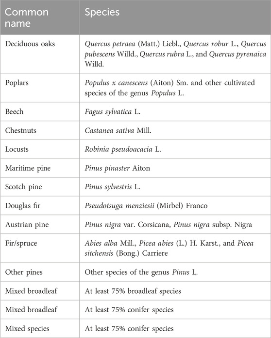
Table 1. Tree species classification.

2.3.2 High-resolution map of tree height from satellites

We used a new 10-m resolution satellite tree height map of France (Forest Multiple Satellite—Height [FORMS-H]; Schwartz et al., 2023; Schwartz et al., 2024; Fayad et al., 2024) corresponding to 2020 (see Figure 2C) to provide tree height in all steps of the study (see Figure 1). It was obtained from a deep learning model based on multi-stream remote sensing measurements (NASA’s GEDI LiDAR mission and ESA’s Copernicus Sentinel-1 and 2 satellites), and it does not use any ground measurements for calibration. The accuracy of FORMS-H has been evaluated with respect to the NFI height for 2020 over all of France (MAE = 2.94 m) and two ALS heights from high definition LiDAR measurements (MAE = 3.54 m and MAE = 4.50 m).

2.3.3 Historical forest disturbance maps

We used the European forest disturbance dataset at a resolution of 30 m built by Senf and Seidl (2021), hereafter S&S, derived from Landsat satellite data (see Figure 2D), to compute an age map of forests by 2020 (see Figure 1). We assumed that the selected disturbances were all severe enough to replace the previous stand (i.e., disturbance intensity greater than or equal to 0.95) and were followed by regrowth. The forest age was computed as the difference between 2020 and the year of disturbance.

2.3.4 National Forest Inventory plots

We used plot data from the French NFI (see Figure 2B) (IGN, 2005) from 2017 to 2021 to provide tree height and age (see Figure 1). The French NFI consists of temporary plots distributed throughout the country on a systematic grid of 1 by 1 km surveyed over a 10-year rotation and made up of three concentric plots of radii of 6, 9, and 15 m. Dendrometric measurements are collected on the 6-, 9-, and 15-m circles for trees with diameters greater than 7.5 cm, 22.5 cm, and 47.5 cm, respectively. For each size class and tree species, a representative tree is selected for the plot, and a height measurement is taken. The dominant height of the plot is the average height of the tallest trees on the plot. Two trees chosen from the six tallest in the plot are cored at a height of 1.30 m to the pith for age measurement by counting annual rings. A general description of the stand including the vertical structure and tree species is established using a 25-m radius plot. We filtered out the trees that are not in the target population. We corrected the age values at 1.30 m to take into account the missing tree rings at heights between 0 and 1.30 m using calibrating measurements from the NFI made in 2005. In order to select the even-aged plots, we selected only the plots with a regular vertical structure with or without understory. In addition, we computed the mean and standard deviation of the distribution of the age per plot, and we selected the plots with a coefficient of variation of age smaller than 0.25 knowing that we kept the plots with single age data. The age of the plot is the average age of the trees within the plot.

2.3.5 Environmental variables

We used 125 environmental variables from various datasets (see Figure 1C). Specifically, we incorporated 14 climatic features, encompassing temperature (Ninyerola et al., 2000; Bertrand et al., 2011; Richard, 2011), precipitation (Ninyerola et al., 2000; Richard, 2011), solar radiation (Lebourgeois and Piedallu, 2005; Piedallu and Gégout, 2007; 2008; Richard, 2011), evapotranspiration (Bertrand et al., 2011), climatic water budget (Piedallu and Gégout, 2007; Piedallu and Gégout, 2008), and the maximum and available water capacity (Al Majou et al., 2008; Piedallu et al., 2011; Piedallu et al., 2013). From the digital elevation model at a resolution of 25 m, we computed the aspect, the slope, the hillshade, and the roughness, leading to five altimetry features with the altitude (IGN, 2017). The 92 soil composition features include a 1-km forest soil pH map and composition data on various soil properties, texture components, essential nutrients, and minerals at a resolution of 16 km (Antoni et al., 2011). The geology of the soil is characterized by eight features (BGRM, 2017). The human impact on growth was taken into account by four features: the private or public ownership of the forest stand, whether the forest stand is in a national park or reserve, and the proximity to roads (i.e., an estimation of skidding distance) (IGN, 2022) and urban areas (IGN, 2018c).

2.4 Consistency of satellite and NFI data

This section makes forest attributes such as height, age, and species consistent across satellite observations and ground-based NFI measurements (see Figure 1A). The BDF tree species and the FORMS-H height were extracted at the precise localization of the NFI plots. Similarly the S&S age map was collocated with the NFI plots and compared with the associated NFI age. The NFI tree species was compared to the corresponding BDF tree species.

2.5 Fitting height–age growth curves for post-disturbance recovery

In this section, we explain how height–age relationships were derived for individual species (see Figure 1B). First, the FORMS-H height and S&S age pixels were assigned to a species from the corresponding BDF stand (dataset I). We then used the BDF map to assign a species to each NFI height and age combination to maintain consistency with the satellite data (dataset II).

2.5.1 Chapman–Richards equation

Growth curves (height–age relationships) per species were computed from all triplets (height, age, and tree species) across the region using space-for-time substitution. For each tree species, the percentile-based growth curves denoted by ${P G C}_{i} (t)$ were computed from the 5th, 25th, 50th, 75th, and 95th percentiles of the height distribution. For each tree species, the percentiles of the height distribution were computed for each 1-year age bin of dataset I and for each 10-year bin of dataset II (see Figure 3A), leading to polymorphic growth curves. For tree species with fewer than 34 data points in dataset II, we refrained from calculating percentiles and utilized the raw data instead. For each tree species, we thus obtained percentile-based growth curves denoted by ${P G C}_{i} (t)$ for the ith percentile. The Chapman–Richards Eq. 1 was then fitted to each ${P G C}_{i} (t)$ . An offset $h_{0}$ parameter was added to take into account the possible overestimation of ground height at young ages (Beck et al., 2020; Dubayah et al., 2020).

P G C (t) = a {(1 - e^{- b t})}^{c} + h_{0} . (1)

Figure 3

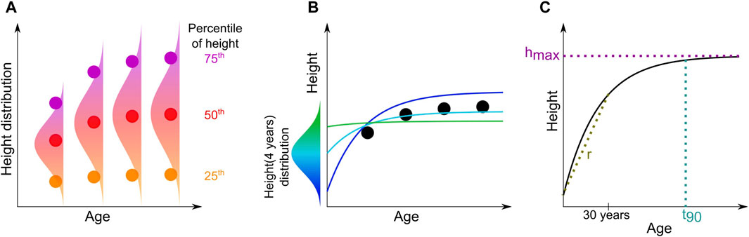
Figure 3. Conceptual figure of the growth curve processing per species (A). For each age bin, a percentile of the height distribution is computed, leading to percentile growth curves (PGCs) (shown as disks). Chapman–Richards fitting with an offset $h_{0}$ (B). The Chapman–Richards equation is fitted to each PGC (disks). The offset $h_{0}$ is set to a value equal to a centile of the height distribution at an age of 4 years, leading to different fitted curves for each centile (lines). The chosen offset value affects the goodness of fit. The offset value that maximized the coefficient of determination averaged across all tree species is chosen. Metrics characterizing tree growth (C). Maximum height $h_{\max}$ , the time $t_{90}$ for which the growth curve has reached 90% of the maximum height, and the early growth rate r defined by the rate of height change in the first 30 years.

To ensure a robust fit, we fixed the offset value $h_{0}$ based on both the tree species and the growth curve percentile, reducing the number of adjustable parameters to three. Specifically, we selected the value of $h_{0}$ based on the height distribution [denoted as h(4)] corresponding to the smallest age bin (4 years) (see Figure 3B). For each tree species and percentile growth curve ${P G C}_{i} (t)$ , we used Eq. 1 to fit the combined datasets I and II while varying $h_{0}$ in 1-percentile increments of h(4). We used the Levenberg–Marquardt algorithm via the curve_fit function in the Python SciPy library for this optimization. The final choice of $h_{0}$ , which maximized the coefficient of determination averaged across all tree species, was determined by analyzing how the coefficient of determination varied with the percentile of h(4) for each quantile regression. Specifically, we set $h_{0}$ as follows: the minimum value of h(4) for ${P G C}_{5}$ , ${P G C}_{25}$ , and ${P G C}_{50}$ ; the 65th percentile of h(4) for ${P G C}_{75}$ ; and the 94th percentile of h(4) for ${P G C}_{95}$ . We used the trust region reflective algorithm implemented in the curve fit function of the Python SciPy library with bounds equal to [0,40], [0.001,1], and [0.1,100] for the fitting parameters a, b, and c, respectively.

2.5.2 Consistency of satellite and NFI data

In order to check the consistency between satellite-derived and field-measured height–age relationships (see Figure 1A), a Chapman–Richards equation was fitted to the median growth curve ${P G C}_{50}$ using three methods based on different combinations of datasets I and II: (M1) dataset II alone, (M2) dataset I + dataset II, the latter only for ages beyond the satellite era (tree age >34 years), and (M3) dataset I + dataset II for all ages. Then, the same Chapman–Richards equation was fitted to each ${P G C}_{i} (t)$ for all tree species using M3.

2.5.3 Growth metrics

Using the fitted parameters, we derived three simple metrics to compare growth curve characteristics between species: the maximum height $h_{\max} = a + h_{0}$ , the time for which the growth curve has reached 90% of the maximum height $t_{90} = \frac{- 1}{b} \ln (1 - {(0.9 - 0.1 \frac{h_{0}}{a})}^{\frac{1}{c}})$ , and the early growth rate defined by the rate of change in height in the first 30 years $P G C (30) / 30$ (see Figure 3C).

2.6 Explainable machine learning model for predicting height

Height variability between locations is not only dependent on age and species but also on the variability of environmental factors and management practices, which are included in a model based on interpretable machine learning (see Figure 1C). We opted for a random forest architecture due to its versatility and robustness as a machine learning algorithm (Breiman, 2001; Khajavi and Rastgoo, 2023; Zhu et al., 2023). The resilience of random forest to noisy and collinear data (Yue et al., 2023) allowed us to compute feature importance (Ishwaran and Lu, 2019), which we used to identify the key environmental variables affecting tree height.

We used the satellite-derived FORMS-H height map as a dependent variable and the S&S age map derived from forest disturbance analysis, the BDF tree species map, and 125 environmental parameters from various French datasets as predictors (see Table 2). We converted the S&S age map into aggregated patches and computed the S&S disturbed patches areas and the intensity of disturbance averaged over the patch, which were also used as predictors (see Table 2). A 10-m buffer was drawn inside the S&S disturbance patches, and the S&S age and disturbed patch area maps, along with the FORMS-H height data and the tree species map from BDF resampled at a resolution of 20 m, were collocated with the 125 environmental variables, resulting in dataset I. The tree species from the BDF and the tree height and age from the NFI were extracted using spatial consistency between the NFI plots and the BDF stands. Then, the 125 environmental variables maps were collocated with the center of the grid associated with the NFI plots, leading to dataset II. One-hot encoding was used to encode the categorical features. We included an additional feature to indicate whether the data originated from dataset I or II.

Table 2

Table 2. Datasets used in the study.

2.6.1 Recursive feature elimination

The fused dataset (dataset I + dataset II) was split into training and test subsets, ensuring that the ratios of tree species and age remained the same in each split. We built a random forest predicting height using all the features and optimized the hyperparameters. Then, using the training subset and the Python scikit-learn implementation of RandomForestRegressor with the parameters n_estimators = 100, max_depth = 15, max_features = 0.5, and criterion = “friedman_mse,” we performed a recursive feature elimination using a 3-fold cross-validation. At each iteration, the feature associated with the lowest feature importance computed is eliminated. The procedure is monitored by the computation of the coefficient of determination at each step. We computed the feature importance in two ways. First, starting from the 128 features, we computed the feature importance using Gini impurity, leading to a coefficient of determination R² slowly increasing and then quickly decreasing with the number of features (see black data points in Figure 4A). Then, starting from the 29 features associated with the maximum of R², we performed another recursive feature elimination while computing the feature importance using permutation with the R² metric and five repeats (see blue data points in Figure 4A). We observed a slower decrease in R² with the number of features when using permutation feature importance than when using Gini impurity feature importance. The subset of six features obtained by permutation feature importance was chosen as this subset corresponds to the smallest importance exceeding 5%. In order to avoid overfitting, the parameter max_depth was then set to 11 for the final model.

Figure 4

Figure 4. Recursive feature elimination. (A) Coefficient of determination R² versus the number of features obtained from the recursive feature elimination. The mean values of R² (markers) and the standard deviation (filled color) correspond to the 3-fold distribution after each step corresponding to the elimination of the least important feature. The feature importance has been computed using the Gini impurity (black) and permutation importance with the R² metric (blue). The red dashed line corresponds to six features. (B–D) Performances of the random forest models with 128 features (B), 29 features (C), and 6 features (D). Density plots of the predicted height versus the true height, with brighter colors indicating a higher density of points. The dashed line represents the 1:1 axis. Distributions and error between the true and predicted heights. The boxplots show the variation in the error with the true height. The median value is represented by a red line, while the upper and lower quartiles are represented by the upper and lower edges, respectively. The whiskers symbolize the 5th and 95th percentiles.

2.6.2 SHAP values

In order to analyze the sensitivity of each of the six explanatory variables on the simulation of tree height, we used SHAP (Lundberg and Lee, 2017; Lundberg et al., 2020). SHAP is a game-theoretic approach that attributes the contribution of each feature to the prediction of a model for a specific instance. The SHAP values indicate the difference induced by a specific feature value to the predicted height with respect to the mean predicted height (Lundberg and Lee, 2017). Consequently, we can assess the significance of various features. The SHAP interaction values differentiate between the main effect term and the interactions of a pair of features (Lundberg et al., 2020). The remaining effects or main effects of a feature are defined as the difference between the SHAP value and the off-diagonal SHAP interaction values. For each tree species, we randomly sampled 500 rows of data, each from different BDF stands from the test subset. For the tree species with an insufficient number of stands, the number of data is the number of rows. The error metrics on this sample are MAE = 3.92 m and R² = 0.103, which are similar to the metrics computed over the whole test subset. We computed the SHAP values and the SHAP interaction values for the 4,134 data using the SHAP Python package. The expected mean value of the model is 11.34 m. The feature importance was computed by permutation with respect to the R² metric with 30 repeats on the same subset used for the SHAP analysis. The SHAP feature importances were obtained using the sum of the absolute SHAP values per feature scaled by the sum over the features (L1 norm).

3 Results

3.1 Consistency of satellite and NFI data

We compared the tree species of the NFI plots and the BDF, the height derived from satellites with that observed at the NFI plots, and the age inferred from S&S with that reported for NFI plots. The BDF species classification is not very coherent with the NFI observations: the sample-weighted F1-score (i.e., harmonic mean of precision and recall) is 0.45. Hence, we used the BDF tree species in the following for the NFI data. For height consistency, the results (see Figure 5A) are very good and comparable with an error of 2.94 m obtained over the whole of France (Schwartz et al., 2023). For age (see Figure 5B), the mean absolute error on the stand age between S&S and NFI is 11 years, but it becomes 6 years (Senf and Seidl, 2021) when removing plots with at least one forest edge and a tree cover smaller than 40% (see Figure 5B). The presence of forest edges and the low tree cover density are likely to introduce bias into the age estimation for the NFI. Furthermore, given that the median patch area is 4 30-m pixels, it is likely that these errors are due to geolocalization errors and edge effects of the disturbed patches.

Figure 5

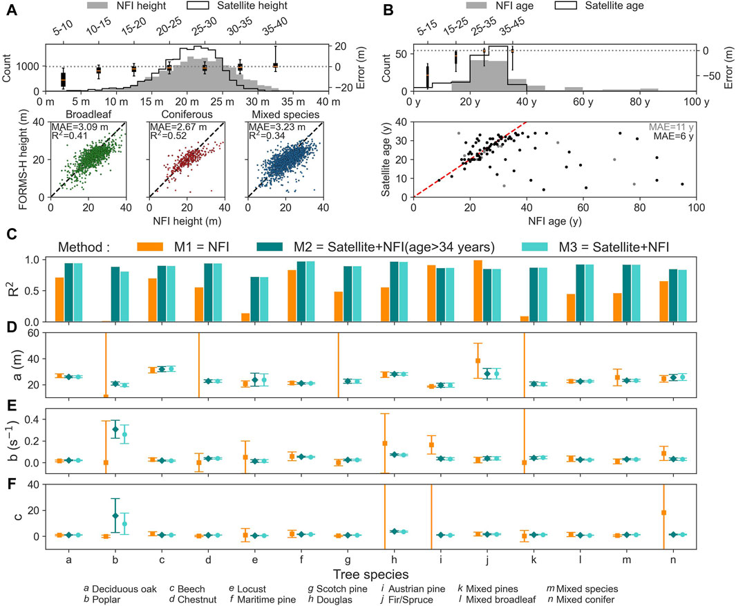
Figure 5. Comparison of satellite-derived height and age with those obtained from the NFI and consistency of growth curves across satellite and NFI data. (A) Distribution, error, and density plots of the satellite (FORMS-H) height versus the NFI height. (B) Distribution, error, and density plots of the satellite (S&S) age versus the NFI age. The dashed line represents the 1:1 axis. Data points likely resulting from geolocation errors and edge effects and the associated MAE are in gray. The median value is represented by a dotted line, while the upper and lower quartiles are represented by the upper and lower edges, respectively. The whiskers symbolize the 5th and 95th percentiles. Coefficient of determination R² (C) and fitted parameters (A–F) for the 14 tree species associated with the Chapman–Richards equation fitted to the median growth curve ${P G C}_{50}$ . The fitting uncertainty on the fitted parameters is displayed by the whiskers.

We compared the growth curves based on the three curve fitting methods explained in Section 2.4. While R² is similar for M2 and M3, it is significantly lower for M1. Nevertheless, the fitted parameter values are similar between the three methods when considering the error margins (see Figures 5C–F). This result suggests that combining satellite, NFI height, and age allows us to better define the shape of the growth curves at young ages rather than using only the NFI data. The satellite data are consistent with the NFI reported values whether or not they are used together in the fit. Based on this, we adopted M3 for defining the “best” growth curves shown in Section 3.2.

3.2 Polymorphic growth curves per species

The height–age patterns for five broadleaf species, six coniferous species, and other mixed forests are shown in Figure 6. While the growth of deciduous oak, mixed broadleaf, and mixed species is described by a large number of points in both datasets, species such as chestnut, locust, fir/spruce, mixed pines, and mixed conifer lack NFI data to constrain their long-term growth. From a visual assessment of the growth curves (see Figure 6), beech, Douglas, Austrian pines, and fir/spruce seem to have an almost linear growth. The growth of beech and Douglas appears to reach the largest height, larger than that of oak, locust, chestnut, and maritime and Austrian pines. Poplars stand out due to their fast initial growth, which is the opposite of oak, beech, Scotch pine, and mixed broadleaf. For Douglas fir, Austrian pine, and fir/spruce stands, the low number of measurements at ages higher than 50 years does not permit us to depict or to estimate the asymptotic value of the maximum dominant height.

Figure 6

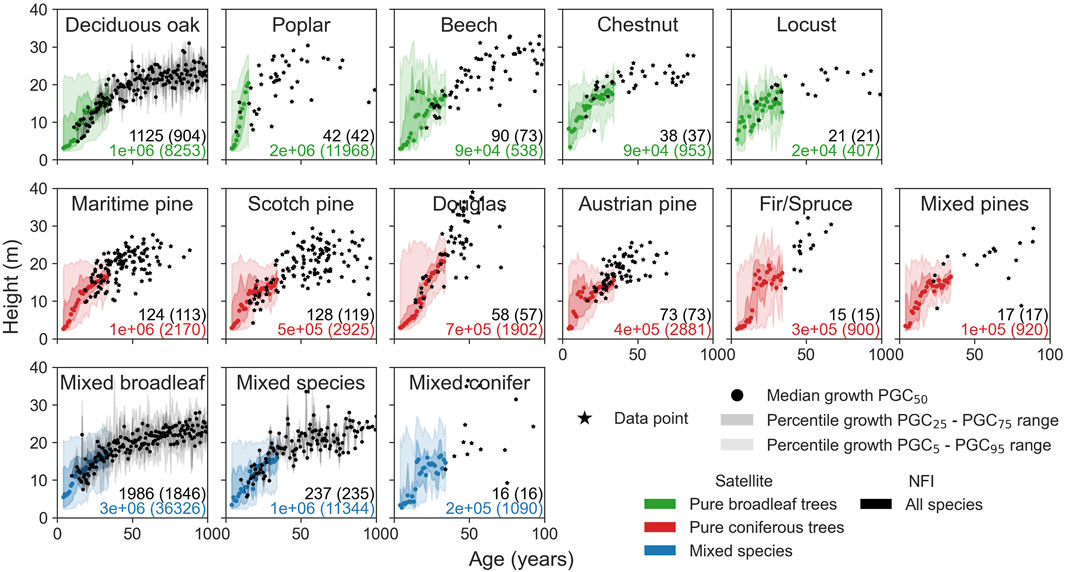
Figure 6. Growth curves for different tree species. Satellite data are in color (green for pure deciduous trees, red for pure coniferous trees, and blue for mixed species), and NFI data are in black. The median (dots), interquartile range (dark filled color), and the interval between the 5th and 95th quantiles (light filled color) are shown for satellite data and deciduous oak, mixed broadleaf, and mixed species of NFI data. For the other tree species of NFI data, the black points correspond to the data points. The numbers of 10-m pixels (left number) and BDF stands (right number in parentheses) are given in black for the NFI data and in color for satellite data.

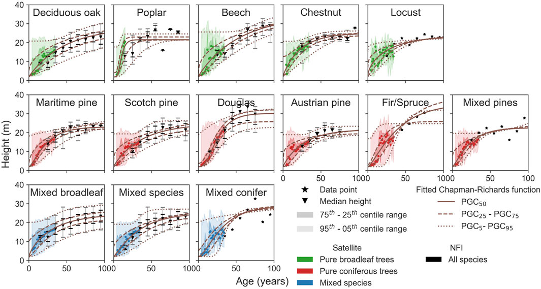
Then, we compared the growth curves after fitting the data with Eq. 1, fit parameters, and metrics from Section 2.5 (see Figure 7). The fitting yielded accurate results: R² averaged over the five percentile growth curves ( ${P G C}_{i}$ ) and the 14 tree species is 0.77, with the smallest values corresponding to tree species associated with a small number of data points.

Figure 7

Figure 7. Fitted growth curves, height versus age, for different tree species. The satellite data are in color (green for the pure deciduous trees, red for the pure coniferous trees, and blue for the mixed species). The NFI data have been digitized into 10-year ranges. ${P G C}_{50}$ is denoted by the black markers, and the black (gray, resp.) whiskers symbolize the ${P G C}_{25}$ and ${P G C}_{75}$ ( ${P G C}_{5}$ and ${P G C}_{95}$ , respectively) percentiles. The fitted Chapman–Richards functions are shown in solid brown for PGC₅₀, dashed brown for ${P G C}_{25}$ and ${P G C}_{75}$ , and dotted brown for ${P G C}_{5}$ and ${P G C}_{95}$ .

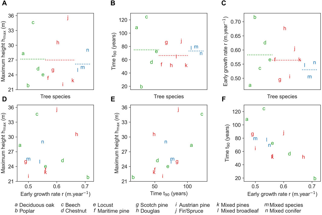
The growth metrics are not significantly different on average between deciduous trees, conifers, or a mixture of both (see Figures 8A–C): when comparing coniferous and deciduous species, we observe similarities in both $h_{\max}$ and early growth rate r. However, $t_{90}$ is smaller on average for conifers than for broadleaves. The early growth rate of mixed species is also not distinguishable from that of conifers and deciduous trees. Our three growth metrics, however, are not independent. While $h_{\max}$ and early growth rate r are not correlated (R² = 0.01, p = 0.96 in Figure 8C), they are both correlated to $t_{90}$ (see Figures 8D–F). The higher the maximum height, the longer the time it takes to reach it. Conversely, the greater the early growth rate r, the shorter $t_{90}$ , regardless of what that $h_{\max}$ may be (see Figures 8D–F). An analogous analysis yields similar results when comparing the metrics of the growth curves ${P G C}_{5}$ , ${P G C}_{25}$ , ${P G C}_{75}$ , and ${P G C}_{95}$ .

Figure 8

Figure 8. Growth metrics associated with the median growth curve PGC₅₀. Maximum height $h_{\max}$ (A), time $t_{90}$ for which the growth curve has reached 90% of the maximum height (B), and early growth rate r (C) for broadleaf species (green), coniferous (red), or mixed species (blue) corresponding to the fitted parameters of the median growth curve ${P G C}_{50}$ . The mean growth metrics for broadleaf, conifer, or mixed species are represented by a horizontal line. Maximum height $h_{\max}$ versus early growth rate r (D). Maximum height $h_{\max}$ versus time $t_{90}$ (E). Time $t_{90}$ versus early growth rate r (F).

3.3 Key features to explain height variations

The growth curves (see Figure 6) suggest a first-order impact of the age and tree species in determining spatial variations in the height of forests. Using explanatory machine learning, we identified other features that might explain variations in height, confirming a dominant role for age and species that Figure 4 suggests. While the coefficient of determination R² of the random forest model prediction decreases with the number of features (see Figure 4A), the mean absolute errors and the coefficients of determination using 128 features, 30 features, or 6 features are similar (see Figures 4B–D). The model with six features is almost as good at predicting the height as the models using more features, and it predicts height from satellite and NFI data with similar precision (MAE = 3.32 m and R² = 0.47 for dataset I; MAE = 3.20 m and R² = 0.53 for dataset II). On average, for different tree species, the model performs with a MAE of 3.38 m and R² of 0.43 with standard deviations of 0.39 m and 0.11, respectively. The six selected features are mostly uncorrelated (see Figure 9A). From the permutation feature importance (see Figure 9B), the main driver to the estimated height is tree age (49%), followed by disturbed patch area, which is defined as the area of the patch within a stand impacted by a disturbance (19%), tree species (10%), and the environmental parameters such as soil pH (9%), altitude (8%), and summer climatic water budget (SCWB) (5%). The impact of the patch area also depends on the tree species (see Figure 10). For small patches, the distribution of values is shifted toward larger values and more diffused than for larger patches.

Figure 9

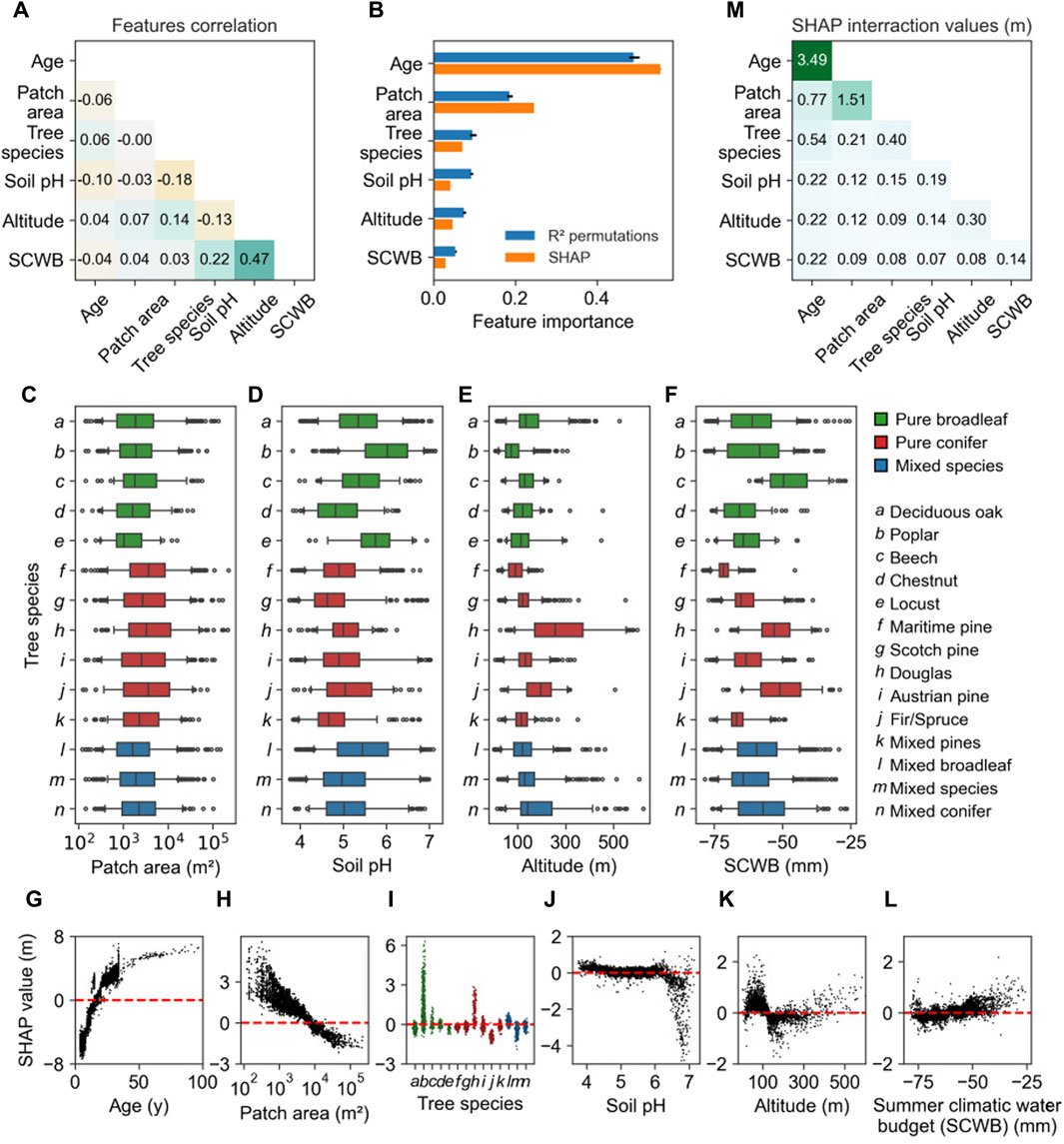
Figure 9. Impact of the six features on the predicted forest height. Correlation of the features (A). Feature importances of the six-feature model computed using permutation and the R² metrics and SHAP values (B). Boxplot of the distributions of the disturbed patch area (C), soil pH (D), the altitude (E), and the summer climatic water budget (SCWB) (F) for each tree species. The data correspond to the data used to compute the SHAP values and interaction values. The median value is represented by a black line, while the upper and lower quartiles are represented by the upper and lower edges, respectively. The whiskers indicate the 5th and 95th percentiles. SHAP value versus feature value for the following features: age (G), disturbed patch area (H), tree species (I), soil pH (J), altitude (K), and SCWB (L). The expected height value of 11.34 m is represented by a dashed red line. Sum of the absolute value of the SHAP interaction values (M).

Figure 10

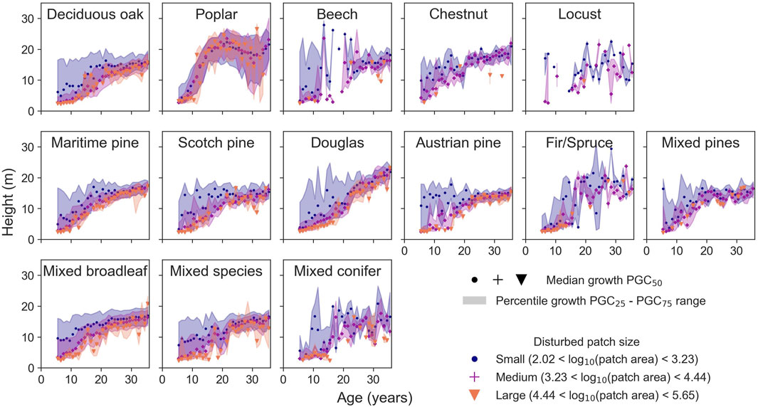
Figure 10. Growth curves for different tree species and disturbed patch areas. The median (markers) and interquartile range (filled color). The disturbed patch areas are categorized into small (blue), medium (purple), and large (orange).

The influence of environmental variables on height estimates is constrained by their range of variation across the study region, illustrated by the distributions of the disturbed patch area, soil pH, the altitude, and SCWB (see Figures 9C–F). Except for the patch area, the distributions of the features are different between species. We investigated the impact of the features on the model height estimates using Shapley indexes (Lundberg and Lee, 2017), hereafter referred to as SHAP. The feature importances from permutation and SHAP analysis are similar (see Figure 9B). The SHAP values correspond to the first-order impact of the features on the height (see Figures 9G–L). The effect of tree age (see Figure 9G) shows that the model reproduces well the exponential growth of the forest (Bontemps and Duplat, 2012; Pretzsch, 2020). The model predicts larger heights when the disturbed area is smaller (see Figure 9H). Except for poplars and, to a lesser extent, Douglas firs and fir/spruces, the SHAP values do not depend much on the tree species (see Figure 9I). Soil pH only has a decreasing impact if the soil pH is sufficiently basic (see Figure 9J). The altitude has a non-monotonous effect on the model output (see Figure 9K). The predicted height increases with the SCWB (see Figure 9L). The second-order impact of features on the predicted height, which is how one feature influences the importance of another, was investigated using the SHAP interaction values (Lundberg et al., 2020) (see Figure 9M). Mainly, the forest age has a strong interaction with the disturbed patch area (see Figure 11, cells 1,2 and 2,1). The growth of poplars and Douglas stands out from the growth of other tree species (see Figure 11, cell 3). For most tree species, the predicted height decreases when the disturbed patch area increases, but the effect is reversed for poplars (see Figure 11, cell 3,2).

Figure 11

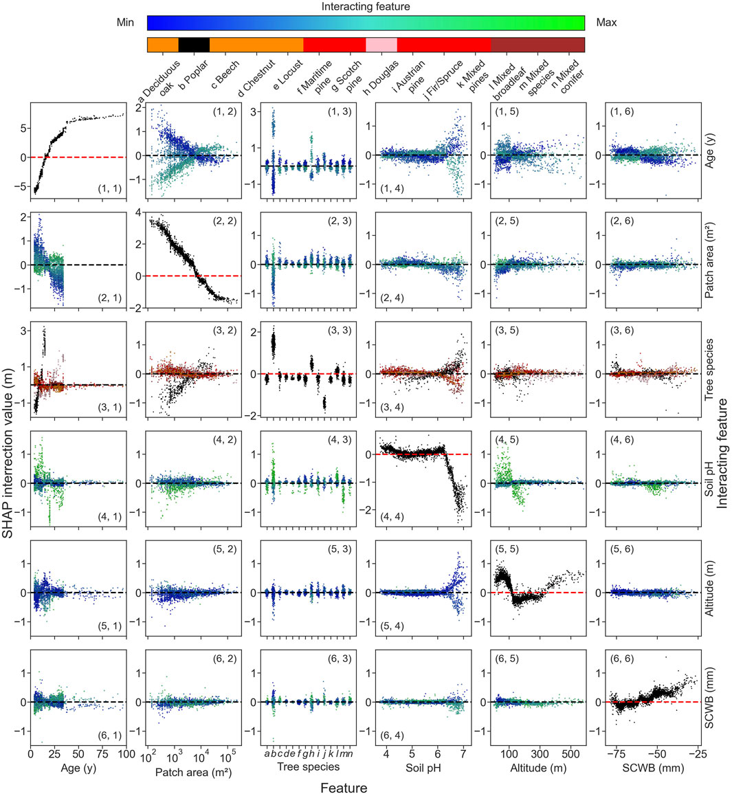
Figure 11. SHAP interaction value between two features. SHAP interaction value versus one feature value, with the interacting feature value highlighted on the off-diagonal and remaining SHAP effect on the diagonal for the following features: age (1), disturbed patch area (2), tree species (3), soil pH (4), altitude (5), and SCWB (6). For the age and the disturbed patch area, the color map is in the logarithmic scale. The expected height value of 11.34 m is represented by a dashed line.

4 Discussion

This study combines data obtained from field measurements and satellite observations to derive height–age growth curves and retrieve well-known drivers of height. The consistency between satellite and NFI data is to be noted as a main result. The combination of satellite and field data enhances the result accuracy (Hasenauer et al., 2012; Neumann et al., 2015; Næsset et al., 2020; Breidenbach et al., 2021).

The growth curves derived from the satellite and NFI data are in agreement with similar results found in the literature for broadleaf (Crockford and Savill, 1991; Álvarez-González et al., 2010; Bontemps et al., 2012; Rédei et al., 2014; Pretzsch et al., 2015; Viet et al., 2023), conifer (Aughanbaugh, 1960; Lemoine, 1991; Zhang et al., 1993; Bravo-Oviedo et al., 2004; Cieszewski et al., 2007; Pretzsch et al., 2010; Pretzsch et al., 2015), or mixed species (Pretzsch et al., 2010; Pretzsch et al., 2015; del Río et al., 2016). Studies of the growth of mixed tree species show a slower early growth than that of pure species, which is in line with our results (del Río et al., 2016). The similarity in height between pure and mixed forests in our results can be attributed to the irregular canopy height and low density, which is not accurately captured at a resolution of 10 m (Pretzsch and Schütze, 2016; Aldea et al., 2021). The effects of tree species on growth cannot be aggregated into a single broadleaf/coniferous/mixed species group. To date, a number of studies calculating height or biomass have used the broadleaf/coniferous distinction alone to take into account the effect of tree species, thus creating a source of uncertainty (Santoro and Cartus, 2023; Schwartz et al., 2023).

Our random forest model predicts forest height with an accuracy (MAE = 3.20 m for 128 features) comparable to the accuracy of the satellite height map FORMS-H (MAE = 2.94 m with respect to the NFI and MAE = 3.54 m or 4.50 m with respect to LiDAR HD measurements). Hence, the accuracy of the model is not reduced by the simplicity of its architecture because it is already constrained by the uncertain height values from FORMS-H.

Apart from the age and tree species features that were expected to be the main predictors of height, our feature elimination procedure selected three environmental variables (soil pH, altitude, and summer climatic water budget) and the disturbed patch area. Other features such as the difference between public and private forests and the proximity to roads and cities had a negligible impact on the height prediction. Low relief and a well-developed road network enable forest management throughout the region (Aguiar et al., 2021). Moreover, proximity to urban areas such as the Île-de-France region (12 million inhabitants for 12,000 km²) does not seem to influence forest growth much (Stone and Skelly, 1974; Pregitzer et al., 2021; Franceschi et al., 2023). The potential management differences, highlighted by the forest ownership and whether the stand is in a natural park, may not be very noticeable since private forests are subject to all types of management, from intensive cultivation to complete neglect. The ownership of the forest and the state park features were not found to be important, likely because this feature inadequately portrays management practices, such as thinning or selective logging.

The importance of the disturbed patch area on the height model may be explained by the fact that the tree age is based on the hypothesis that the forest starts to grow back immediately after the disturbance. While poplar stands are mostly planted after cutting, natural regeneration prevails for the majority of other tree species (IGN, 2020), which is in agreement with our results. In contrast, natural regeneration is impacted by the micro-climate and the preservation and dispersion of seeds, in part driven by the disturbed patch area (Parde, 1962; d Oliveira and Ribas, 2011; Hanbury-Brown et al., 2022).

Overall, our model accurately predicts the most favorable soil pH condition for the selected tree species to reach a higher height at a given age (Hjelm and Rytter, 2016; Cremer and Prietzel, 2017; Arrobas et al., 2018). Since the SCWB, which corresponds to the amount of rainfall available to plants once evaporation and transpiration needs have been met, is always negative (see Figure 9F), the trees draw on soil reserves to survive the summer. Notably, in the process of recursive feature elimination, the SCWB was chosen over summer available water capacity (SAWC), which quantifies the water available to plants. Since water supplies are rarely insufficient in the studied area, the accessibility of water to trees is primarily constrained by rainfall. The susceptibility of beech (Weber et al., 2013; Leuschner, 2020), Douglas (Sergent et al., 2014; Chauvin et al., 2019), fir/spruces (Solberg, 2004; Lévesque et al., 2013), and Scotch pines (Bigler et al., 2006; Eilmann et al., 2009; Martínez-Vilalta et al., 2012) to drought aligns with the reports of previous research. The other species demonstrate an ability to withstand drought conditions proficiently (Eilmann et al., 2009; Lévesque et al., 2013). Mixed-species categories encompass the effects of multiple species not specifically identified by the BDF and the impacts of mixed species, making it difficult to conclude.

Different biases are associated with the satellite-derived and ground measurement data: since the BDF was computed from images spanning 10 years, it is possible that the recent disturbances have led to a change in the tree species. The historical S&S disturbance map only indicates one disturbance event between 1984 and 2020, providing no insight into the age homogeneity of the resulting forest. Additionally, its 30-m resolution is coarse, potentially leading to boundary effects.

An indirect space-for-time approach was used to obtain the growth curves. Assuming that the productivity of each forest site does not vary over time, temporal dynamics were inferred by studying multiple sites that differ under abiotic conditions not directly related to stand age or time (Fukami and Wardle, 2005). The environmental variables are also supposed to be constant over the last 100 years. Consequently, any application of these models to predict changes in site productivity over time is reliant on the underlying assumption of equivalence between the stands. In the context of climate change, the invariance of the climatic and environmental variables is challenged, potentially compromising our results (Rolo et al., 2016; Wu et al., 2022; Yue et al., 2023).

5 Conclusion

The consistency of the tree height and age derived from satellite and ground measurements is promising for monitoring a forest and its evolution at larger scales, i.e., regional or country level. Here, satellite and ground-based data were found to be consistent, and thus, they were combined to produce the first growth curves per species in a large forested region (question A). The significant variations in tree growth according to tree species cannot be accurately reported by a coarse categorization into broadleaf or conifer (question B). Several environmental factors that are known to influence tree height were identified in addition to tree age and species: soil pH, altitude, and summer climatic water budget. In addition, the post-disturbance growth was shown to be highly dependent on the disturbed area due to different regeneration methods, natural or plantation (question C). At a regional level, our results did not showcase any discernible human impact on tree growth, whether from urban vicinity or different management techniques, likely due to a lack of detailed data, specifically on management types. Management types may also be correlated with other parameters, such as tree species, soil, and climate, which may make it difficult to isolate their effects on tree growth.

Data availability statement

The datasets presented in this study can be found in online repositories. The names of the repository/repositories and accession number(s) can be found at: https://zenodo.org/doi/10.5281/zenodo.10079578.

Author contributions

AP-T: conceptualization, data curation, formal analysis, methodology, validation, writing–original draft, and writing–review and editing. PC: conceptualization, funding acquisition, methodology, writing–original draft, and writing–review and editing. MS: writing–review and editing. IF: methodology and writing–review and editing. YX: formal analysis and writing–review and editing. FR: writing–review and editing. AdT: writing–review and editing. J-ML: writing–review and editing.

Funding

The author(s) declare that financial support was received for the research, authorship, and/or publication of this article. This work was supported by the French German AI4Forest R-22-FAI1-0002-01. AP-T was supported by the ANR project “plan France Relance” with CEA Kayrros.

Conflict of interest

Authors IF and AdT were employed by Kayrros SAS.

The remaining authors declare that the research was conducted in the absence of any commercial or financial relationships that could be construed as a potential conflict of interest.

Publisher’s note

All claims expressed in this article are solely those of the authors and do not necessarily represent those of their affiliated organizations, or those of the publisher, the editors, and the reviewers. Any product that may be evaluated in this article, or claim that may be made by its manufacturer, is not guaranteed or endorsed by the publisher.

References

Aguiar, M. O., Fernandes da Silva, G., Mauri, G. R., Ribeiro de Mendonça, A., Junio de Oliveira Santana, C., Marcatti, G. E., et al. (2021). Optimizing forest road planning in a sustainable forest management area in the Brazilian Amazon. J. Environ. Manage 288, 112332. doi:10.1016/j.jenvman.2021.112332

PubMed Abstract | CrossRef Full Text | Google Scholar

Aldea, J., Ruiz-Peinado, R., del Río, M., Pretzsch, H., Heym, M., Brazaitis, G., et al. (2021). Species stratification and weather conditions drive tree growth in Scots pine and Norway spruce mixed stands along Europe. For Ecol Manag 481, 118697. doi:10.1016/j.foreco.2020.118697