Suitability of different in-water algorithms for eutrophic and absorbing waters applied to Sentinel-2 MSI and Sentinel-3 OLCI data

Optically complex waters present significant challenges for remote sensing due to high concentrations of optically active substances (OASs) and their inherent optical properties (IOPs), as well as the adjacency effect. OASs and IOPs can be derived from atmospheric correction processors’ in-water algorithms applied to data from Sentinel-2 MultiSpectral Instrument (S2 MSI) and Sentinel-3 Ocean and Land Color Instrument (S3 OLCI). This study compared S3 OLCI Level-2 in-water products for Case-2 waters with alternative in-water algorithms derived from ACOLITE, POLYMER, C2RCC, and A4O. Fifty in-water algorithms were evaluated using an extensive match-up dataset from lakes and coastal areas, focusing particularly on small lakes with high colored dissolved organic matter absorption at 442 nm (up to 48 m^-1). The Chl a band ratio introduced by Gons et al. (2022) applied to data processed by ACOLITE performed best for S3 OLCI Chl a retrieval (dispersion = 23%, bias = 10%). Gons et al. (2022) band ratio also showed consistent agreement between S3 OLCI and S2 MSI resampled data (intercept of 6.27 and slope of 0.83, close to the 1:1 line); however, lower Chl a values (<20 mg/m³) were overestimated by S2 MSI. When estimating errors associated with proximity to land, S2 MSI Chl a in-water algorithms had higher errors close to the shore (on average 315%) compared to S3 OLCI (on average 150%). Chl a retrieved with POLYMER had the lowest errors close to the shore for both S2 MSI and S3 OLCI data (on average 70%). Total suspended matter (TSM) retrieval with C2RCC performed well for S2 MSI (dispersion 24% and bias −12%). Total absorption was most accurately derived from C2RCC applied to S3 OLCI L1 data (dispersion < 43% and bias < −39%), and it was better estimated than its individual components: phytoplankton, mineral particles, and colored dissolved organic matter absorption. However, none of the colored dissolved organic matter absorption in-water algorithms performed well (dispersion > 59% and bias < −29%).

1 Introduction

The inherent optical properties (IOPs) of water, such as absorption and scattering, significantly influence the underwater light field and water color. These IOPs depend on the type, composition, and concentration of optically active substances (OASs) in the water. OASs can be divided into three groups, namely, phytoplankton and its main pigment chlorophyll-a (Chl a), total suspended matter (TSM), and colored dissolved organic matter (CDOM), each interacting differently with light. Chl a has absorption peaks in the blue (440–500 nm) and red (650–680 nm) regions of the visible light spectrum (Kirk, 2011). TSM includes two fractions: suspended particulate inorganic matter (SPIM) and suspended particulate organic matter (SPOM). SPIM, composed of mineral particles, mainly scatters light, while SPOM, which includes phytoplankton cells, non-living cellular matter, zooplankton, and organic detritus, both scatters and absorbs light, sharing a similar absorption spectrum shape to CDOM. CDOM, resulting from decaying organic material (Coble, 2007), absorbs light most significantly in the blue region of the visible light spectrum, with absorption decreasing exponentially toward longer wavelengths (Mobley, 1994; Mobley, 2022). Waters where IOPs are influenced solely by phytoplankton are classified as Case-1 waters. Conversely, waters where IOPs are significantly influenced by other OASs, besides Chl a, such as TSM and CDOM, are classified as Case-2 waters (Morel and Prieur, 1977). These are called optically complex waters.

Remote sensing reflectance (Rrs) is the primary parameter derived from ocean color satellite data. Secondary products, such as optical water quality parameters, are obtained from Rrs using various methods, including modeling, empirical algorithms, and semi-analytical algorithms. Rrs can be derived through an inverse model using IOPs, which include total absorption and total backscattering coefficients. Total absorption is the sum of the absorption by phytoplankton, CDOM, TSM, and pure water, while total backscattering is the sum of the backscattering by water, mineral particles, and organic particles. OAS concentrations and IOPs can be retrieved from Rrs(λ) using a forward model; different modeling methods are summarized by Yang et al. (2022). Chl a concentration is a proxy, for example, for quantifying phytoplankton biomass and monitoring potentially toxic algal blooms (Duckey et al., 2006). Chl a is also used to apply the bi-directional reflectance model to derive water reflectance from water remote sensing products (Morel et al., 2002; EUMETSAT, 2021a). Sediment resuspension increases TSM concentrations in water, impacting IOPs and the underwater light field (Baker and Lavelle, 1984). TSM also plays a crucial role in geophysical and biological processes in water, such as flocculation, heavy metal transport, and phytoplankton blooms (Dyer et al., 2000; Pannard et al., 2007; Burd and Jackson, 2009; Bourrin et al., 2021). CDOM can be used as a proxy for dissolved organic carbon to understand the carbon cycle (Osburn et al., 2016) and identify organic pollution in urban and agricultural catchments (Tzortziou et al., 2015). Monitoring these parameters on a large scale helps assess water quality. Phytoplankton pigment concentration, via Chl a absorption, can be used as a proxy for phytoplankton biomass and as an indicator of primary productivity (Marra et al., 2007), despite the large variation present in the Chl a/phytoplankton biomass relationship due to various light and nutrient conditions (Kasprzak et al., 2008). CDOM’s absorption at specific wavelengths (usually at 412 or 442 nm) (a_CDOM(412) or a_CDOM(442)) allows estimating CDOM absorption from satellite data and calculating its concentrations. Backscattering and scattering are proxies of TSM concentrations in areas where detritus dominates water’s optical properties (Reynolds et al., 2016). The backscattering ratio provides indices on suspended particle size distributions, origin, and composition (Woźniak et al., 2018). The quantities of OASs and nutrients affect water quality. For example, Chl a concentrations can indicate the trophic state of lakes: oligotrophic waters (<2.6 mg/m³) are considered to have good quality; mesotrophic waters (2.6–20 mg/m³), moderate quality; eutrophic waters (20–55 mg/m³), poor quality; and hypereutrophic waters (>55 mg/m³), very poor quality (Istvánovics, 2009). Eutrophication, driven by nutrient loads in the water, leads to increased phytoplankton blooms and is a vast problem (Downing, 2014; Huisman et al., 2018). Therefore, monitoring water constituents to estimate and improve water quality is vital.

Measuring water constituents and IOPs directly from water samples is time-consuming and costly. Remote sensing offers advantages with its spatial and temporal resolution, enabling more efficient monitoring (Schaeffer et al., 2013; Wang and Yang, 2019; Yang et al., 2022). Monitoring lakes and coastal areas using satellite data is challenging due to atmospheric components, OASs in the water, and the vicinity of the land affecting water pixels. Copernicus Programme’s Sentinel-2 (S2) and Sentinel-3 (S3) A/B with continuous C/D satellites ensure continuous availability of data for environmental monitoring at least until 2035 (ESA, 2016; ESA, 2021). The S2 MultiSpectral Instrument (MSI) has a spatial resolution of up to 10 m, with radiometric and spectral resolutions initially designed for land applications but effectively used for water quality monitoring (Du et al., 2016; Toming et al., 2016; Grendaitė et al., 2018; Ansper and Alikas, 2019; Giardino et al., 2019; Bhangale et al., 2020; Sent et al., 2021). The S3 Ocean and Land Color Instrument (OLCI) has more suitable radiometric and spectral resolutions for ocean color monitoring, but its spatial resolution of 300 m could not be sufficient for small lakes (Pirasteh et al., 2020; Soomets et al., 2020).

The atmospheric correction (AC) procedure is essential for deriving Rrs and has been validated in many studies (Warren et al., 2019a; Mograne et al., 2019; Pahlevan et al., 2021). However, since Rrs is the basis for deriving OAS and IOPs, AC processors also generate these parameters using processor-based in-water algorithms. These algorithms have not been validated with a large amount of match-up data. According to the S3 mission requirements document (Drinkwater and Rebhan, 2007), accuracy requirements for Case-1 and Case-2 waters have been established for OASs and water-leaving reflectance. When deriving Chl a, TSM, and CDOM products for Case-2 waters, the accuracy should be at least 70%, with a goal of 10% accuracy. In addition to S3 OLCI Level-2 (L2) Rrs and water quality products, alternative AC processors suitable for S2 MSI and S3 OLCI data have been developed. These include the POLYnomial-based approach established for the atmospheric correction of MERIS data (POLYMER) (Steinmetz et al., 2011) and ACOLITE (Vanhellemont and Ruddick, 2018), both of which derive OASs and are applicable to both S2 MSI and S3 OLCI. The Case-2 Regional Coast Color (C2RCC) algorithm (Brockmann et al., 2016), suitable for both S2 MSI and S3 OLCI, and Atmospheric Correction for Optical Water Types (A4O) (Hieronymi et al., 2017) for S3 OLCI derive OAS and IOPs. Since water pixels are influenced by the vicinity of the land, the capability of AC processors to work under these conditions should be considered during the validation of in-water algorithms (Bulgarelli et al., 2014; Bulgarelli and Zibordi, 2018b).

In this work, we focus on algorithms whose application limits can, in principle, include the local conditions but not, for example, on algorithms that have been optimized for the open ocean. We have a number of in situ measured concentrations of water constituents and associated inherent optical properties from lakes with a relatively high Chl a and CDOM concentration. We compare some water algorithms that derive these parameters directly from satellite data based on the recommendations of the original developers; there may be other algorithms or combinations of AC and water retrieval that are not considered here. Therefore, the objectives of the study are to 1) compare OASs and IOPs derived from AC processors’ in-water algorithms with in situ measured data; 2) determine whether the distance from the shore is associated with the errors between in situ and satellite data; and 3) determine the consistency of in-water algorithms between S2 MSI and S3 OLCI.

2 Materials and methods

2.1 Area of interest

The study area comprises Estonian lakes and the Baltic Sea, which are optically complex waterbodies (Figure 1). Lake Peipsi, a shallow and well-mixed transboundary lake between Estonia and Russia, is Estonia’s largest lake (3,555 km²) and the fourth largest in Europe (Kapanen, 2018). Lake Peipsi is divided into three parts: the largest, mesotrophic Peipsi sensu stricto (s.s.) in the north; the hypertrophic Lake Pihkva in the south; and the eutrophic Lake Lämmijärv, which connects the northern and southern parts. Cyanobacterial blooms occur annually in the summer–autumn period. Lake Võrtsjärv, Estonia’s second largest lake (270 km²), is a shallow, very turbid, well-mixed, and non-stratified waterbody (Nõges and Nõges, 2012). Forty small lakes across Estonia were used for match-up analysis, ranging from relatively clear waters with low quantities of OASs (e.g., Secchi depth of 5 m) to extremely absorbing waters with high a_CDOM(442) (48 m^-1) (e.g., Secchi depth of 0.3 m, data collected by Tartu Observatory’s water remote sensing team). Their depths varied from 1 to 38 m (Keskkonnaagentuur, 2024). Match-up data were gathered from two areas of the Baltic Sea: Pärnu Bay, a shallow bay in south-western Estonia dominated by TSM and CDOM (Paavel et al., 2011), and the Western Gotland Basin (Kyryliuk and Kratzer, 2019) near the Swedish coast, where the water depth at measurement sites was approximately 30 m.

Figure 1

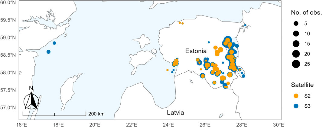
Figure 1. Locations of OAS and IOP match-up data in Estonia and the Baltic Sea. S2 MSI match-up data are shown in dark yellow, and S3 OLCI match-up data are shown in blue. The size of the circle indicates the number of concurrent match-ups between in situ measurements and satellite overpasses during the study period from 2015 to 2022.

2.2 In situ data

OASs varied on a large scale in the studied waterbodies. Chl a concentrations ranged from 1.5 to 341 mg/m³ (average 24.8 mg/m³), TSM concentrations ranged from 0.005 to 143.3 mg/L (average 9 mg/L), and a_CDOM(442) ranged from 0.4 to 48 m^-1 (average 3.8 m^-1). The maximum values of the in situ OAS in match-ups for each AC were 125 mg/m³ (C2RCC, L2, POLYMER, and ACOLITE) and 30 mg/m³ (A4O) for Chl a; 143 mg/L (C2RCC), 34 mg/L (L2), and 14 mg/L (A4O) for TSM; and 5 m^-1 (A4O) and 43 m^-1 (C2RCC) for a_CDOM(442 nm). The summary statistics of all measured in situ data are provided in Supplementary Table S1.

The majority of water samples were gathered from the surface layer (all small lakes and coastal waters). However, during the national monitoring of Lakes Peipsi and Võrtsjärv, integrated water samples were gathered. Lake Võrtsjärv, being shallow, turbid, and well-mixed, showed no difference between surface and integral water samples. In Lake Peipsi, differences in Chl a and TSM concentrations occurred at deeper points during specific conditions, such as quiet weather and algal blooms, when surface concentrations were higher than integral values. Nevertheless, this was a negligible amount compared to the general number of match-ups. As for the match-up points, where both surface and integral samples were collected during specific optics field work accompanying national monitoring activities, the surface sample was finally used. Sampling was performed according to ISO 5667-3 (The International Organization for Standardization, 2018), and laboratory analyses were performed according to ISO 10260 (The International Organization for Standardization, 1992). Water samples were filtered through pre-combusted Whatman GF/F filters to obtain TSM concentrations, which were then measured gravimetrically after drying (1 h at 104°C). The precision of the weights of the filter for TSM was 0.01 mg. SPIM was measured gravimetrically after combustion at 550°C for 30 min. SPOM was obtained by subtracting SPIM from TSM (ESS, 1993).

For Chl a concentration, water samples were filtered using Whatman GF/F filters and refrigerated at −20°C until measurements. Pigments were extracted for 24 h with 5 mL of 96% ethanol, centrifuged for 10 min at 4,000 rpm, measured using Hitachi U-3010 UV-VIS (Hitachi, Japan) and PerkinElmer LAMBDA UV/VIS (PerkinElmer, USA) spectrophotometers, and calculated according to Jeffrey and Humphrey (1975).

Absorption coefficients of phytoplankton pigments (a_pig(442)) and non-algal particles (a_NAP(412 and 442)) and total absorption (a_tot(442)) were measured in the laboratory using a Hitachi U-3010 UV-VIS Spectrophotometer with a Spectralon^®-coated integrating-sphere attachment using the method by Tassan and Ferrari (1995).

a_CDOM(412 and 442) as with a_NAP were retrieved after filtration of the filtrate using a Millipore filter (pore size 0.2 µm) and measured using the Hitachi U-3010 UV-VIS Spectrophotometer.

The calculations of scattering and backscattering coefficients in the studied waterbodies are detailed by Uusõue et al. (2022). Total scattering (b_tot(442)) and particle scattering (b_part(442)) were calculated from absorption and attenuation coefficients measured using WETLabs AC-S (WETLabs, USA), following the user manual (WET Labs, 2011). Backscattering coefficients were calculated from the volume scattering function measured with WETLabs ECO-VSF3 (WETLabs, USA) at three wavelengths (470, 532, and 660 nm), following the user manual (WET Labs, 2007). The particle backscattering coefficients (b_bpart) at specific wavelengths (510 and 550 nm) were obtained by interpolation. Phytoplankton and mineral mass-specific scattering coefficients (b_phyto(442) and b_mineral(442) m²/g) were obtained by dividing the scattering coefficients by SPOM and SPIM concentrations, respectively (Snyder et al., 2008).

2.3 Satellite data

S2 MSI Level-1 (L1) and S3 OLCI L1 and L2 full-resolution (FR) non-time critical data were downloaded for the period 2016–2022:

• S2 A/B MSI data were downloaded from the Copernicus Open Access Hub (https://scihub.copernicus.eu) with processing baselines of 02.04–04.00.

• S3 A/B OLCI L1 data were downloaded from the EUMETSAT Data Store (https://data.eumetsat.int) for 2016–2019 (reprocessed) and 2021–2022, or from the EUMETSAT Data Centre (https://archive.eumetsat.int/) for 2020 with processing baseline 002. L2 data were downloaded from the EUMETSAT Data Store (https://data.eumetsat.int/) for 2016–2020 (reprocessed) and 2021–2022 with processing baseline 003.

L1 data for both S2 MSI and S3 OLCI were processed using ACOLITE, C2RCC, and POLYMER processors. S3 OLCI data were additionally processed with A4O. For S2 MSI L1 data, IdePix (9.0.2) (Wevers et al., 2021) was additionally used to identify invalid pixels before applying the C2RCC AC processor. S3 OLCI A/B FR data (300 m) and S2 MSI A/B (10 m) were extracted for match-up analyses. Processor-based flagging was used (Supplementary Table S2). A description of AC processors’ products for deriving OASs and IOPs is shown in Table 1, and the background of each product is provided in the references. A brief description of the AC processors, their methodologies, and in-water algorithms is provided in the following sections.

Table 1

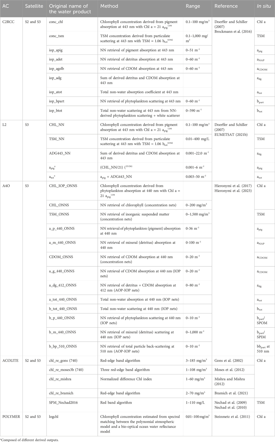
Table 1. Overview of selected water quality parameters from satellite data with applied atmospheric correction and description of underlying methods. C2RCC and L2 contain the same processing chain and bio-geo-optical models with only minor differences. C2RCC/L2 and A4O-ONNS use the entire visible Rrs spectrum but with slightly different band configurations. ACOLITE-based water algorithms utilize red and red-edge bands.

C2RCC (v2.1) consists of a processing chain of several neural networks (NNs) and is designed for optically complex Case-2 waters (Doerffer and Schiller, 2007; Brockmann et al., 2016). Although originally developed for MERIS, it can be used for S2 MSI, S3 OLCI, and other satellite missions. The basis for the NNs is large amounts of simulated training data for radiative transfer in the atmosphere and water. In the NN atmospheric correction process, the water-leaving reflectance is estimated from the top-of-standard-atmosphere reflectance. The water part uses an NN that estimates five IOPs at 443 nm from the water-leaving reflectance spectrum; these IOPs are the absorption coefficient of phytoplankton pigments at 443 nm (a_pig), the absorption coefficient of detritus at 443 nm (a_det), the absorption coefficient of CDOM (also known as gelbstoff) at 443 nm (a_CDOM), and the scattering coefficients of particles (b_part) and a white scatterer (b_whit). Concentrations of Chl a and TSM are derived from these IOPs using bio-geo-optical models with scaling factors determined primarily from measured data from the North Sea and adjacent regions (Röttgers et al., 2023). These parameters are listed in Table 1 but can be adapted regionally. For both S2 MSI and S3 OLCI data, processor-based default settings were used except for salinity, which was changed to 0 PSU in lakes. The NNs for S2 MSI and S3 OLCI are slightly different according to the sensor characteristics.

L2 is the standard S3 OLCI water product for Case-2 waters (*_NN). This is essentially the same processing chain as C2RCC, based on Doerffer and Schiller (2007). Small differences arise due to the use of System Vicarious Calibration gains and the lack of options for influencing salinity and ancillary data (EUMETSAT, 2024). With this alternative processing for Case-2 waters, however, not all products are provided.

A4O-ONNS (v1.0) is a further development of C2RCC. The OLCI Neural Network Swarm (ONNS v0.23) water algorithm uses several NNs that are each optimized for defined optical water types (OWTs) (Hieronymi et al., 2017). It is designed for all natural waters, from clear oceanic to extremely absorbing or scattering waters, and considers diverse phytoplankton communities. The ONNS algorithm was created for S3 OLCI but can be used for other satellite sensors via a band adapter, although not for S2 MSI (Hieronymi, 2019). A4O is a novel atmospheric correction for S3 OLCI by Hieronymi et al. (in prep), which is optimized to exploit the optical water type requirements of the ONNS water algorithm. A4O also consists of an ensemble of NNs to output fully-normalized remote sensing reflectance. Moreover, some unique flags are provided, e.g., to indicate uncertainties in the case of eutrophic waters (floating algae) and possible optically shallow waters (adjacency). Further details of A4O and a comparison with other AC methods are described by Hieronymi et al. (2023). The ONNS water products (Table 1) are derived from various OWT-specific net structures and are essentially based on Hydrolight radiative transfer simulations and bio-geo-optical relationships comparable to C2RCC, but ONNS delivers a few more products that are not part of this inter-comparison, like the diffuse attenuation coefficient of downwelling irradiance, Kd490.

ACOLITE (v20221114.0) uses a dark spectrum fitting method and is designed for turbid Case-2 waters, applicable to both S2 MSI and S3 OLCI. Its methodology involves identifying dark pixels on the image to select the band with the lowest atmospheric top-of-atmosphere reflectance. The processing scheme is image-based and does not require external data, such as aerosol optical thickness, which is calculated based on the dark pixels. Deriving Chl a and TSM parameters is based on calculated water-leaving reflectances, where band ratio algorithms are applied (Table 1). A more detailed processing scheme for calculating water-leaving reflectance is provided by Vanhellemont and Ruddick, (2018) and Vanhellemont (2019). For S2 MSI, the “fixed” option for aerosol optical depth at 550 nm was used, which calculates only one single value for an image previously defined by regions-of-interest (ROIs). For S3 OLCI, the default “tiled” option was used, dividing the image into 6 × 6 km tiles, calculating each tile value, and then interpolating the full image. Additionally, Ancillary and Shuttle Radar Topography Mission Digital Elevation Model data from the Earthdata database (https://earthdata.nasa.gov) were used. Other processor-based settings for both satellites were used as “default.”

POLYMER (v4.16) uses a spectral matching method based on a polynomial model with sun glint removal and an ocean reflectance model, designed mainly as an ocean color product but also suitable for Case-2 waters for S2 MSI and S3 OLCI. For deriving water-leaving reflectance, top-of-atmosphere reflectance is corrected (for gases, ozone, Rayleigh scattering, and sun glint). The spectral matching method is used to obtain the best spectral fit for corrected top-of-atmosphere reflectance. Chl a concentration and the backscattering coefficient of non-covarying particles are derived based on the ocean reflectance model calculating water-leaving reflectance (Morel, 1988). A more detailed description of the processing scheme is provided by Steinmetz et al. (2011). Logchl is a standard Chl a product, which was solved (10 ^logchl), but the product name logchl remained in the study.

The most common in-water algorithms of all ACs were selected to cover a wide range of parameters, retrievable from satellite data (Table 1).

2.4 Match-up protocol and statistics

For match-up analysis, the S3 validation protocol was followed (EUMETSAT, 2021a) for both S2 MSI and S3 OLCI. In situ data were collected on the same day as the satellite overpass. The downloaded satellite data were processed with AC processors and their respective in-water algorithms. Then, 1 × 1 and 3 × 3 ROIs were exported using the Pixel Extraction tool in Sentinel Application Platform (SNAP) (v9.0) software. To compare the consistency between S2 MSI and S3 OLCI data, the S2 MSI products were resampled to 300-m pixel resolution using the Resample tool (v2.0) in SNAP. The comparison was made on 3 × 3 ROIs. Statistical analysis was done using R software (v2022.12.0). Standard deviations for error estimation were calculated for in situ data when multiple measurements were available for one water sample or one measurement station.

For the 3 × 3 ROIs, outliers were removed before further calculations. First, the mean (μ) and standard deviation (σ) of each ROI were calculated. Second, pixels were discarded if they met the conditions provided in Eqs 1, 2.

$\left[pixelvalue\right]<\mu -1.5\sigma ,(1)$

or

$\left[pixelvalue\right]>\mu +1.5\sigma .(2)$

Only ROIs where 50% + 1 pixels (at least five pixels) remained were used for further calculations. Finally, the coefficient of variation (CV) of each ROI was calculated to obtain the final match-ups (Eq. 3).

$CV=\frac{\sigma }{\mu }\times 100\%,(3)$

where μ and σ were calculated for each ROI after eliminating outliers. When CV > 20%, the match-up was discarded.

Uncertainties for the 3 × 3 ROIs were retrieved as average satellite-derived uncertainty values after the elimination of the outliers, which were described above. For 1 × 1 ROIs, uncertainty for one pixel was exported. Not all products had uncertainty values.

The following statistics were calculated between in situ and satellite (S2 MSI and S3 OLCI) data:

The primary metrics used for the validation of the in-water algorithms were errors, estimated using Eqs 4, 5. First, the median percentage error (MdPE) was calculated to estimate the bias, indicating how much the data were underestimated or overestimated by the in-water algorithms (Eq. 4).

$MdPE=\begin{array}{c}median\\ 1\le i\le N\end{array}\left\{\frac{x_{satellite,i}-x_{insitu,i}}{x_{insitu,i}}\right\}\times 100.(4)$

Second, the median absolute percentage error (MdAPE) was calculated to estimate the dispersion of the data around the 1:1 line (Eq. 5):

$MdAPE=\begin{array}{c}median\\ 1\le i\le N\end{array}\left\{\left|\frac{x_{satellite,i}-x_{insitu,i}}{x_{insitu,i}}\right|\right\}\times 100.(5)$

The absolute percentage error (APE) (Eq. 6) was calculated between in situ and satellite match-up data to estimate the difference between the in situ measured and satellite-derived values:

$APE=\left|\frac{\left(x_{satellite}-x_{insitu}\right)}{x_{insitu}}\right|\times 100.(6)$

To analyze the adjacency effect on satellite data, the distance was measured from the in situ point to the closest shoreline.

Linear regression was used to estimate, both visually and quantitatively, with the determination coefficient (R²), slope, and intercept, how well the model predicts satellite-derived parameter values (dependent variables) as a function of observed in situ values (independent variables). Depending on the context, a high R² value (Eq. 7) indicates a good fit of the model to the data. The slope (b₁) shows the steepness of the regression line and how far the data points are from the 1:1 line. The higher the b₁, the steeper the slope, and the farther the data points are from the 1:1 line. The intercept (b₀) shows where the regression line intersects the y-axis of the dependent variable (satellite-derived parameters). The independent variable in that location is 0.

$R^2=1-\frac{{{\displaystyle \sum }}_{i=1}^N{\left(x_{insitu,i}-x_{satellite}\right)}^2}{{{\displaystyle \sum }}_{i=1}^N{\left(x_{insitu,i}-x_{insitu,average}\right)}^2}.(7)$

The slope and intercept can be expressed in the form of a linear equation (Eq. 8) as follows:

$y=b_0+b_{1}x,(8)$

where b₀ is the y-intercept, b₁ is the slope, y is the dependent variable, and x is the independent variable. For all the previous equations, N represents the number of match-ups, x_satellite represents the parameter obtained with the in-water algorithm (S3 OLCI or S2 MSI), and x_{in situ} represents the parameter measured in situ.

Frequencies were calculated to estimate the percentage of the remaining match-ups after the flagging process. Data (1 × 1 pixel) were used for the calculations for all in-water algorithms. The number of match-ups retained by each algorithm was divided by the total match-up data on each parameter specific to each AC.

3 Results

3.1 Water quality parameters

3.1.1 Chl a

Seventeen Chl a in-water algorithms applied to S3 OLCI and S2 MSI data were validated (Table 1). Satellite-derived Chl a concentration was limited to 250 mg/m³ (the maximum in situ Chl a concentration in usable match-ups was 125 mg/m³) to remove large outliers. Indeed, ACOLITE had outliers above 400 mg/m³, reaching 6,000 mg/m³ for both S3 OLCI and S2 MSI. C2RCC had four outliers above 200 mg/m³ for S2 MSI. The dispersion (MdAPE) and bias (MdPE) for 1 × 1 and 3 × 3 ROIs are presented in Table 2, and R², slope, and intercept within the linear equation are shown in Figures 2, 3.

Table 2

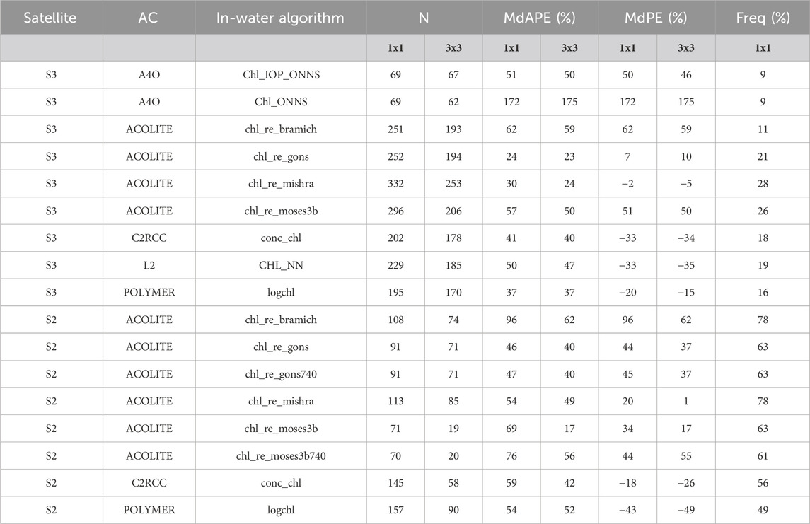
Table 2. Statistics of Chl a in-water algorithms derived from S3 OLCI and S2 MSI 1 × 1 and 3 × 3 ROIs. AC stands for atmospheric correction, N is the number of match-ups, MdAPE is dispersion, MdPE is bias and freq is % of remaining match-ups after applying flags.

Figure 2

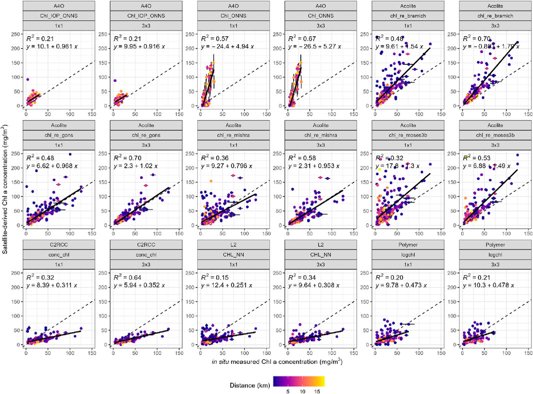
Figure 2. Chl a concentration match-ups derived from S3 OLCI L2 and alternative processing schemes (A4O, ACOLITE, C2RCC, and POLYMER) applied to S3 OLCI L1 data. The satellite-derived Chl a concentration is limited to 250 mg/m³ to eliminate outliers. Horizontal error bars represent the standard deviation of in situ-measured values, and vertical error bars represent satellite uncertainty.

Figure 3

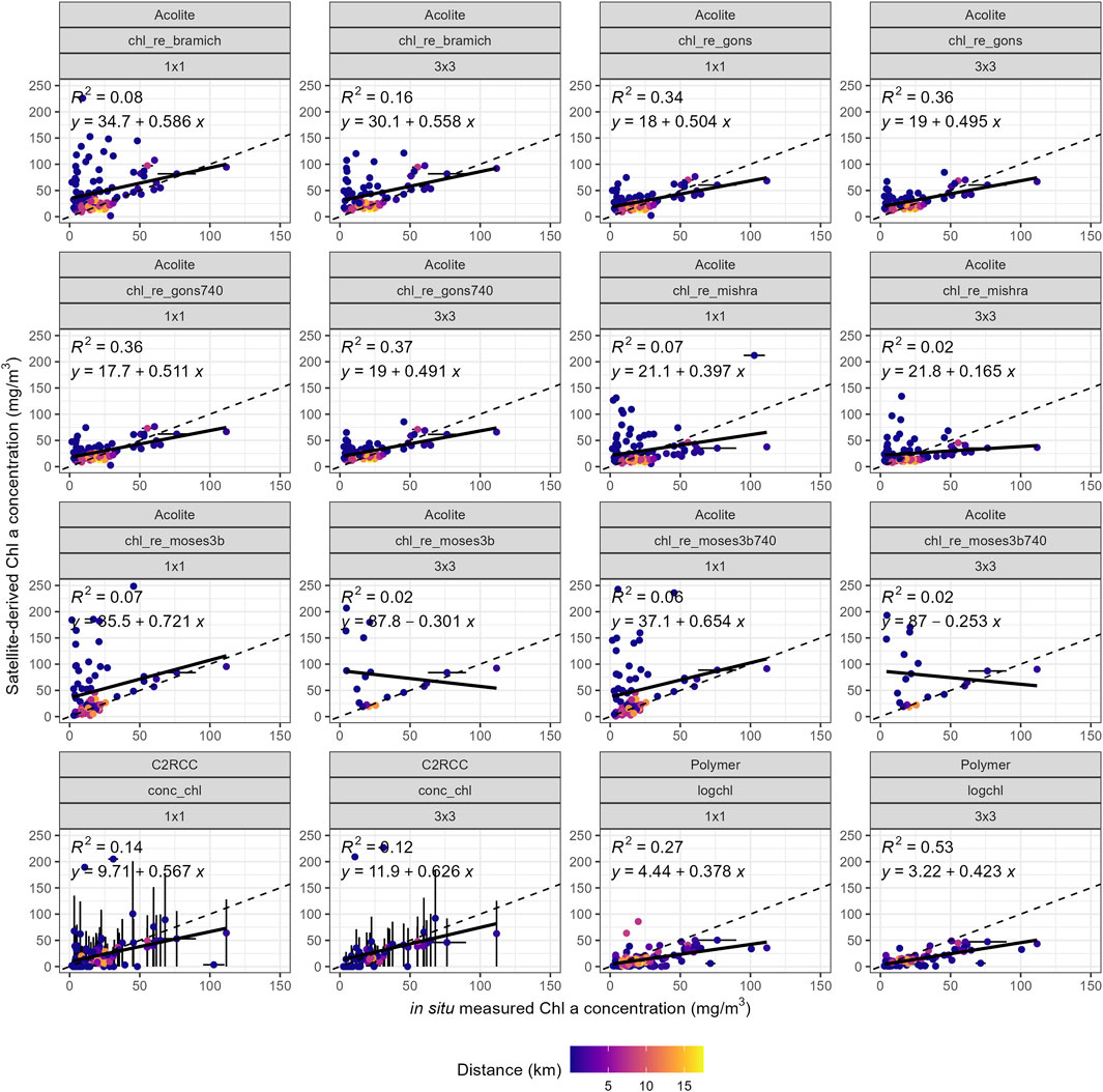
Figure 3. Chl a concentration match-ups derived from in-water algorithms (ACOLITE, C2RCC, and POLYMER) using S2 MSI data. The satellite-derived Chl a concentration is limited to 250 mg/m³ to eliminate outliers. Horizontal error bars represent the standard deviation of in situ-measured values, and vertical error bars represent satellite uncertainty.

Generally, the in situ vs. 1 × 1 ROI data had more outliers, higher error estimates (MdAPE and MdPE), and lower R² values than the in situ vs. 3 × 3 ROI data (Table 2; Figures 2, 3). Therefore, the focus will be on the statistics of 3 × 3 ROIs . The chl_re_gons algorithm (ACOLITE) showed the best accuracy when applied to S3 OLCI and compared to in situ data (Figure 2). This algorithm had the lowest dispersion (MdAPE = 23%) among all the Chl a in-water algorithms, with a slight overestimation (MdPE = 10%) compared to in situ measurements. The dispersion increased for Chl a concentrations above 40 mg/m³. Data aligned closely with the 1:1 line, with a slope of 1.02 and an intercept of 2.30 (R² = 0.70). Similarly, the chl_re_mishra algorithm (ACOLITE) had a slightly higher dispersion than the chl_re_gons algorithm (MdAPE = 24%), particularly for in situ Chl a concentrations above 20 mg/m³. It produced values closely aligned with the 1:1 line, with a slope of 0.95 and an intercept of 2.31 (R² = 0.58). The chl_re_bramich, chl_re_moses3b (ACOLITE), and CHL_IOP_ONNS (A4O) algorithms showed a systematic overestimation (MdPE > 45%). In contrast, the conc_chl algorithm (C2RCC) and CHL_NN product (L2) systematically underestimated Chl a concentrations, especially for concentrations above 20 mg/m³ (MdPE ∼ −35%). The logchl algorithm (POLYMER) showed increased dispersion for in situ values above 20 mg/m³. The chl_ONNS algorithm (A4O) significantly overestimated all Chl a concentrations (MdPE = 175%).

For S2 MSI, all Chl a algorithms exhibited high dispersion (MdAPE up to 62%) in the vicinity of the land, with either underestimation (C2RCC and POLYMER) or overestimation (ACOLITE) (MdPE ranging from −49% to 62%). The accuracy of ACOLITE in-water algorithms tended to improve in more productive waters (Chl a > 25 mg/m³) (Table 2; Figure 3). The slopes were below 0.6, and the intercepts were above 18, showing high dispersion for small Chl a concentrations.

Next, we studied how AC processors were impacted by different flags and analyzed how many match-ups remained for each AC in-water algorithm (frequencies) after applying flags. There are several algorithm-specific flags for invalid pixel expression and additional warnings, although it is often unclear how these are to be used (Hieronymi et al., 2023). Considering retrievals deviating from in situ measurements, we have chosen to apply the available warning flags. This excludes many possible match-ups, especially for A4O near land. For S3 OLCI, low percentage of match-ups remained after applying flags (up to 28%). More than 20% of match-ups remained for each ACOLITE in-water algorithm, while only 9% of match-ups remained for the A4O algorithms. In addition, a low percentage (18% and 19%) of match-ups remained for C2RCC and L2, respectively. For S2 MSI, the remaining match-ups’ frequencies were higher than those for S3, ranging between 49% and 78% (POLYMER and ACOLITE, respectively).

3.1.2 TSM

Five TSM in-water algorithms were validated for S3 OLCI and S2 MSI (Figure 4). All the algorithms applied to S3 OLCI data overestimated TSM concentrations (MdPE > 88%) (Table 3). The TSM_NN product (L2) showed the best accuracy in terms of bias (MdPE = 88%) and dispersion (MdAPE = 88%). TSM concentrations retrieved with the TMS_NN product (L2) and conc_tsm algorithm (C2RCC) were closer to the 1:1 line for in situ values below 10 mg/L (Figure 4A). However, the dispersion increased above 80% for concentrations above 20 mg/L, where most measurements were performed close to the shore (within 5 km). Error bars showed that high TSM concentrations and outliers were associated with high satellite-derived uncertainties. TSM concentrations retrieved with the TSM_IOP_ONNS algorithm (A4O) showed high dispersion (MdAPE = 129%) across all in situ concentration ranges and had 2.5 times fewer match-ups (N = 66) compared to the conc_tsm algorithm (C2RCC) (N = 170) and TSM_NN product (L2) (N = 177).

Figure 4

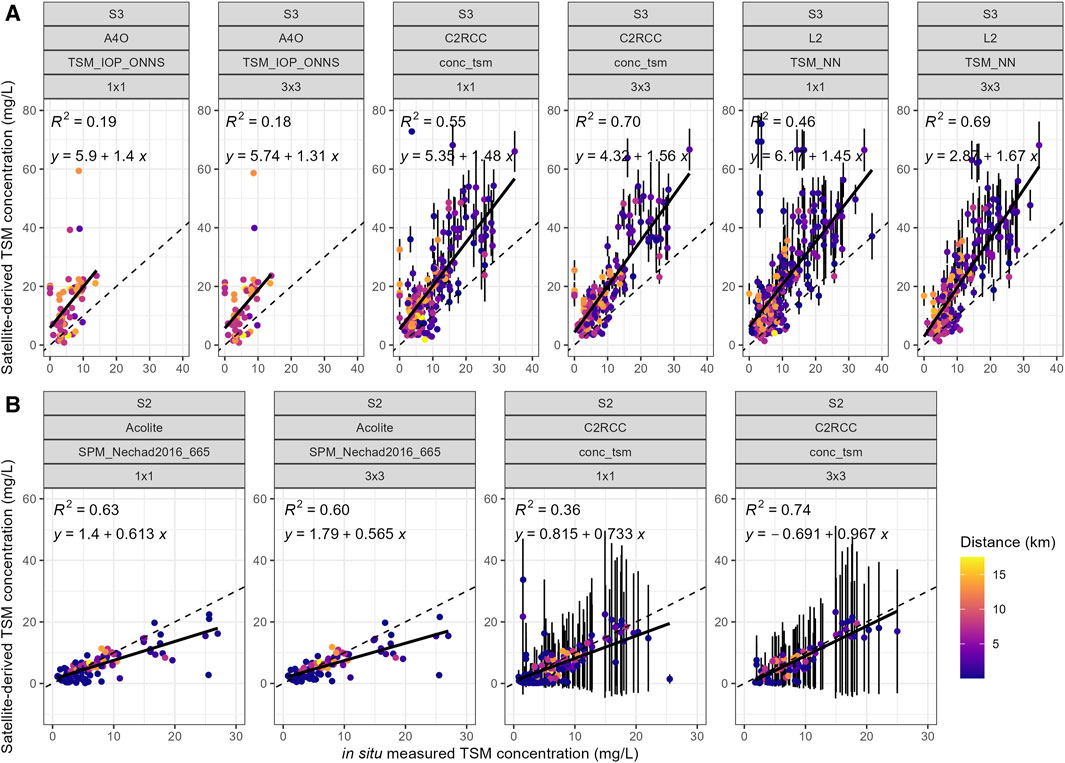
Figure 4. TSM concentration match-ups derived from S3 OLCI L2 and alternative processing schemes (A4O and C2RCC) applied to S3 OLCI L1 data (A) and in-water algorithms (ACOLITE and C2RCC) applied to S2 MSI (B). The satellite-derived TSM concentration is limited to 80 mg/L, respectively, to eliminate outliers. Vertical error bars represent the satellite-derived uncertainty.

Table 3

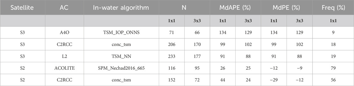
Table 3. Statistics of TSM in-water algorithms derived from S3 OLCI and S2 MSI 1 × 1 and 3 × 3 ROIs. AC stands for atmospheric correction, N is the number of match-ups, MdAPE is dispersion, MdPE is bias and freq is % of remaining match-ups after applying flags.

For S2 MSI, the conc_tsm algorithm (C2RCC) provided the most accurate results, aligning well with the 1:1 line for all values (intercept −0.69, slope 0.97, and R² = 0.74) with an overall dispersion of 24% (Table 3). The SPM_Nechad2016_665 algorithm (ACOLITE) underestimated TSM concentrations (MdPE = −9%), but TSM concentrations below 10 mg/L were close to the 1:1 line.

The analysis of the remaining match-ups after applying flags showed that the highest frequencies were observed with the S2 MSI ACOLITE algorithm (79%), while the lowest frequencies were with the S3 OLCI A4O algorithm (9%). C2RCC performed better on S2 than on S3 when there were 56% and 18% of match-ups, respectively.

3.1.3 IOPs

3.1.3.1 Absorption parameters

Twenty absorption in-water algorithms were validated for S3 OLCI (Figure 5; Table 4) and S2 MSI (Figure 6; Table 4). A description based on the different processing schemes is provided in the following section. a_dg(412 and 443) represented the sum of a_NAP (412 and 443) and a_CDOM(412 and 443).

Figure 5

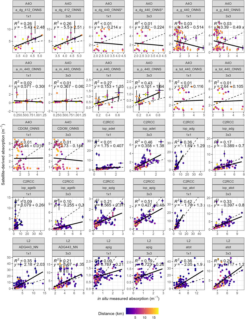
Figure 5. Absorption match-ups derived from S3 OLCI L2 and alternative processing schemes (A4O and C2RCC) applied to S3 OLCI L1 data. Horizontal error bars represent the standard deviation of in situ-measured values, and vertical error bars represent the satellite uncertainty.

Table 4

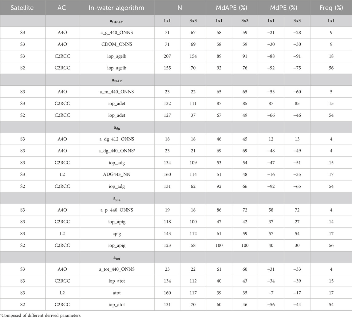
Table 4. Statistics of absorption in-water algorithms derived from S3 OLCI and S2 MSI 1 × 1 and 3 × 3 ROIs. AC stands for atmospheric correction, N is the number of match-ups, MdAPE is dispersion, MdPE is bias and freq is % of remaining match-ups after applying flags.

Figure 6

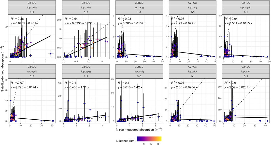
Figure 6. Absorption match-ups derived from the alternative processing scheme C2RCC applied to S2 MSI L1 data. Horizontal error bars represent the standard deviation of in situ-measured values, and vertical error bars represent the satellite uncertainty.

3.1.3.1.1 A4O in-water algorithms

a_pig(440) derived with the a_p_440_ONNS algorithm was the closest to the 1:1 line with an intercept of 0.10 and a slope of 1.64 (R² = 0.43) (Figure 5), but it was systematically overestimated (MdPE = 72%) (Table 4). The a_dg_412_ONNS algorithm underestimated a_dg(412) values below 4 m^-1 and overestimated those above 4 m^-1. Other A4O algorithms, including a_dg_440_ONNS (a_dg(440)) and a_g_440_ONNS calculated from concentration nets (a_CDOM(440)), CDOM_ONNS calculated from IOPs nets (a_CDOM(440)), a_m_440_ONNS (a_NAP(440)), and a_tot_440_ONNS (a_tot(440)), showed high dispersion (MdAPE > 55%), with strong tendencies to underestimation (MdPE < −28%). The correlation of the linear regression was low (R² < 0.3), the slope was between −0.51 and 0.34, and the intercept between −0.26 and 0.34.

3.1.3.1.2 C2RCC in-water algorithms

iop_atot (a_tot(443)) performed better than other C2RCC in-water algorithms for absorption retrieval, with values close to the 1:1 line (a slope of 0.82 and an intercept of −0.40 (R² = 0.33). The iop_atot, iop_adg (a_dg(443)), and iop_agelb (a_CDOM(443)) algorithms systematically underestimated in situ values (MdPE between −39% and −91%). The iop_agelb algorithm had the highest correlation among all a_CDOM(443) in-water algorithms (R² = 0.10). High satellite-derived uncertainties of the iop_atot, iop_adg, and iop_agelb algorithms were associated with outliers that strongly overestimated the in situ values. The iop_adet algorithm systematically overestimated a_NAP(443) values (MdPE = 85%). iop_apig (a_pig(443)) overestimated a_pig(443) values below 1 m^-1 and underestimated a_pig(443) values above 1 m^-1.

3.1.3.1.3 L2 products

The apig (a_pig(443)) product was derived using the CHL_NN (L2) formula (Eq. 9):

$CH{L}_{NN}=21\times {apig}^{1.04}.(9)$

This algorithm overestimated low a_pig(443) values (below 1 m^-1) and underestimated high a_pig(443) values (above 1 m^-1) with high dispersion (MdAPE = 61%). The atot (a_tot(443)) product was derived by adding the apig product to the ADG443_NN product (a_dg(443)). Both atot and ADG443_NN products were well-aligned with the 1:1 line with negative biases (MdPE = −17% and −35%, respectively). Highly overestimated ADG443_NN retrievals were associated with higher uncertainties. Among all absorption parameters, a_tot(443) was derived with the lowest bias (MdPE = −17%) and dispersion (MdAPE = 35%).

For S2 MSI, only the C2RCC algorithms could derive absorption parameters (Figure 6). The iop_apig values were generally close to the 1:1 line (slope of 1.42), but four outliers contributed to the elevated bias (MdPE = 30%) (Table 4). The iop_adet, iop_adg, iop_agelb, and iop_atot algorithms systematically underestimated absorption values (MdPE was below −44%), especially for a_det(443) values above 0.5 m^-1 and a_dg(443), a_CDOM(443), and a_tot(443) values above 10 m^-1. High satellite-derived uncertainties were associated with outliers in the iop_apig, iop_adg, and iop_atot algorithms.

After flagging, C2RCC had the overall highest number of match-ups (> 50%) after applying flags to S2 MSI data. On S3 OLCI, C2RCC flags yielded fewer match-ups compared to S2 MSI (only 15%–18% of match-ups remained). Overall, A4O algorithms yielded the lowest number of match-ups (between 4% and 9%).

3.1.3.2 Scattering parameters

Five in-water algorithms were analyzed to derive scattering parameters for S3 OLCI and S2 MSI.

For S3 OLCI C2RCC, the iop_btot algorithm systematically overestimated b_tot(443) values (MdPE = 308%) (Table 5; Figure 7A). Conversely, the iop_bpart algorithm underestimated b_part(443) values (MdPE = −99%). The A4O in-water algorithms derived only 2–4 match-ups for each parameter (b_bp_510_ONNS, b_m_440_ONNS, b_p_440_ONNS, and b_tot_440_ONNS), making comprehensive statistical analysis challenging. However, Figure 7A shows that A4O in-water algorithms tended to overestimate in situ scattering values.

Table 5

Table 5. Statistics of scattering and backscattering in-water algorithms derived from S3 OLCI and S2 MSI 1 × 1 and 3 × 3 ROIs. AC stands for atmospheric correction, N is the number of match-ups,MdAPE is dispersion, MdPE is bias and freq is % of remaining match-ups after applying flags.

Figure 7

Figure 7. Scattering match-ups derived from alternative processing schemes (A4O and C2RCC) applied to S3 OLCI L1 data (A) and C2RCC applied to S2 MSI L1 data. (B). Horizontal error bars represent the standard deviation of in situ measured values, and vertical error bars represent the satellite uncertainty.

For S2 MSI, only the C2RCC in-water algorithms were available (Figure 7B). The iop_bpart algorithm underestimated b_part(443) values (MdPE = −21%), and iop_btot overestimated b_tot(443) values (MdPE = 105%) (Table 5; Figure 7B).

The analysis of the remaining match-ups after applying flags showed that C2RCC had overall more match-ups with S2 MSI (52%). It had only 12%–33% of match-ups with S3 OLCI. The lowest number of match-ups was obtained with A4O (12%–13%).

3.2 Impact of applying the quality flags

The contribution percentages of the most frequently raised flags are described in Supplementary Table S3. Four groups of AC in-water algorithms were studied: A4O, C2RCC, and L2 applied to S3 OLCI and C2RCC applied to S2 MSI. The highest number of pixels across all algorithms were eliminated with the A4O AC processor (87%–96%), and the ACOLITE AC processor eliminated the smallest number of pixels (21%–39%).

In the case of S3 OLCI, flag contributions were high, up to 93%. The most frequently raised flag for the A4O in-water algorithms was AC_flag_adjacency (pixels influenced by the vicinity of the land). It was raised in 83%–93% of cases for overall match-ups. AC_flag_floating (pixels influenced by the floating algae) was raised in 22%–56% of cases, and AC_flag cloud_risk (risk of cloud presence on pixels) was raised in 37%–57% of cases. For C2RCC, the most frequently raised flag was Cloud_risk (risk of cloud presence on pixels (51%–63%)). Rtosa_OOS (spectral shape of top-of-atmosphere radiance not known by the C2RCC NN) was raised in 18%–50% of cases, Rhow_OOS (spectral shape of water leaving reflectance input spectrum to the IOP retrieval neural net is out of training range) in 38%–60% of cases, and Quality_flag_sun_glint_risk (potential presence of sun glint on pixels) in 8%–19% of cases. Other flags had a negligible effect. The most highly contributing flag for L2 in-water algorithms was WQSF_lsb_OCNN_FAIL (pixels on which the NN algorithm failed), which was raised in 51%–57% of cases. WQSH_lsb_CLOUD_MARGIN (pixels influenced by cloud edges) was raised in 20%–21% of cases. Other flags’ contribution was between 1% and 7%—WQSF_lsb_CLOUD_AMBIGOUS (pixels identified with possible clouds, semi-transparent clouds), WQSF_lsb_AC_FAIL (pixels with a suspect baseline atmospheric correction), and WQSF_lsb_HIGHGLINT (pixels with a non-reliable sun glint correction).

In the case of S2 MSI, flag contributions were low (below 32% of cases). The Cloud_risk flag (risk of cloud presence on pixels) had the highest contribution for C2RCC, being raised in 25%–32% of cases. IDEPIX_POTENTIAL_SHADOW (pixels influenced by potential cloud shadow) was raised in 14%–21% of cases. IDEPIX_LAND (pixels identified as land pixels) were raised in 11%–13% of cases; however, these pixels were located in the water but close to shore.

3.3 Errors associated with the vicinity of the land

To estimate errors associated with the vicinity of the land, APE (Eq. (6)) was calculated for each match-up (3 × 3 ROI vs. in situ value) for all Chl a products (Figure 8). S2 MSI (Figure 8A) and S3 OLCI (Figure 8B) data were analyzed separately for better visualization. The highest errors were observed near shore (<5 km) for S2 MSI and S3 OLCI data. Errors decreased as the distance from the shore increased (>5 km), dropping to below 100%. Therefore, distance groups were chosen as <5 km and >5 km, representing equally distributed data.

Figure 8

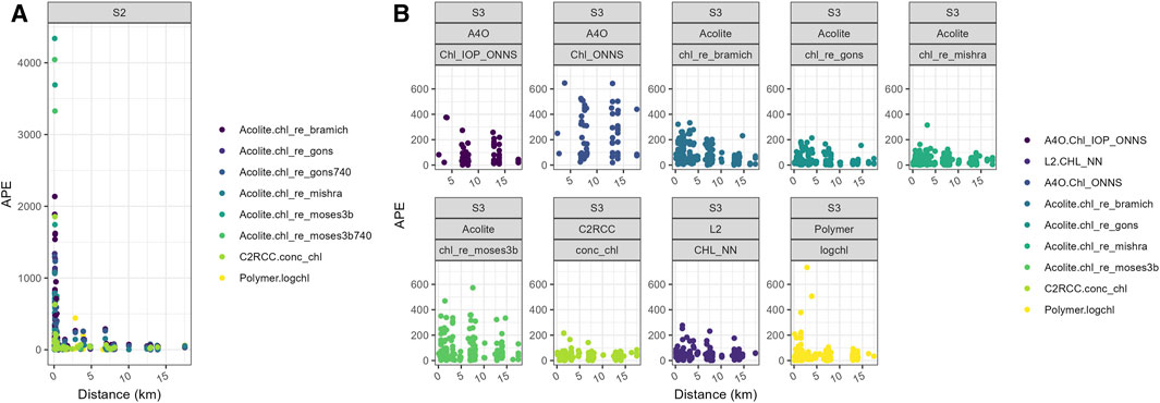
Figure 8. Errors (APE %) of S2 MSI (A) and S3 OLCI (B) associated with the vicinity of the land in all Chl a in-water algorithms based on 3 × 3 ROI. S3 OLCI errors were limited to 750%.

Mean errors (mean APE %) were calculated for each Chl a in-water algorithm based on the distance group. The mean errors were higher for the distance group close to the shore (<5 km) (S2 MSI: 315% and S3 OLCI: 150%) and lower for the group farther from the shore (>5 km) (S2 MSI: 35% and S3 OLCI: 80%), except for the S3 OLCI chl_re_moses3b algorithm (ACOLITE), where the mean error increased (Figure 9). Comparing the mean errors of S2 MSI and S3 OLCI for Chl a in-water algorithms between near-shore and offshore locations, the difference was higher for S2 MSI (∼280%) than for S3 OLCI (∼70%). The mean errors for S3 OLCI were less than 100% in both distance groups, except for the Chl_ONNS algorithm (A4O). The mean errors for S2 MSI were less than 100% close to shore and more than 100% farther from the shore. Only the logchl algorithm (POLYMER) showed mean errors of less than 100% in both distance groups for both S2 MSI and S3 OLCI, with a difference in the mean error of approximately 30% between the two groups. The highest difference in mean error between distance groups was observed for the ACOLITE algorithms (∼360%) for S2 MSI and A4O algorithms (∼311%) for S3 OLCI.

Figure 9

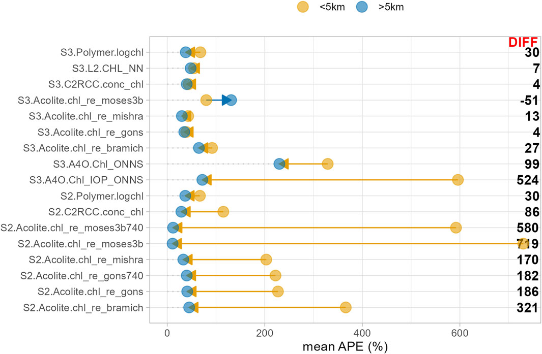
Figure 9. Mean error (mean APE %) differences of S2 MSI and S3 OLCI in-water algorithms in two distance groups: <5 km (dark yellow) and >5 km (blue) based on 3 × 3 ROI data. Arrows indicate the trend of mean APE changes between the two distance groups.

3.4 S2 MSI vs. S3 OLCI

The consistency of 12 in-water algorithms between S3 OLCI (3 × 3 ROI) and S2 MSI (resampled to 300 m, 3 × 3 ROI extraction) was analyzed by comparing match-up data with in situ measurements (Figures 10A, C). Differences between satellite data and in situ data were also compared based on the distance from the shore (Figures 10B, D). Error bars represent the standard deviation of 3 × 3 ROIs. The ACOLITE Chl a in-water algorithms showed a high correlation (R² > 0.8) between S3 OLCI and S2 MSI data. The chl_re_gons algorithm (ACOLITE) had a slope of 0.8 and an intercept close to 6, with values close to the 1:1 line. However, lower Chl a concentrations (less than 20 mg/m³) were overestimated by S2 MSI compared to S3 OLCI. In situ Chl a concentrations were overestimated (up to approximately 10 mg/m³) by both S2 MSI and S3 OLCI. The chl_re_mishra (ACOLITE) (R² = 0.83) and chl_re_bramich (ACOLITE) (R² = 0.93) algorithms also exhibited a high correlation between S3 OLCI and S2 MSI, but with low slopes of 0.4 and 0.6, respectively (intercept greater than 8). Higher Chl a concentrations (more than 20 mg/m³) were underestimated by S2 MSI compared to S3 OLCI. Most of the Chl a concentrations derived by chl_re_bramich (ACOLITE) applied to both S2 MSI and S3 OLCI were overestimated by approximately 10 mg/m³ over all Chl a values compared to in situ measured Chl a. Chl a derived by chl_re_mishra (ACOLITE) applied to both S2 MSI and S3 OLCI had most similar values to in situ measured Chl a with some outliers.

Figure 10

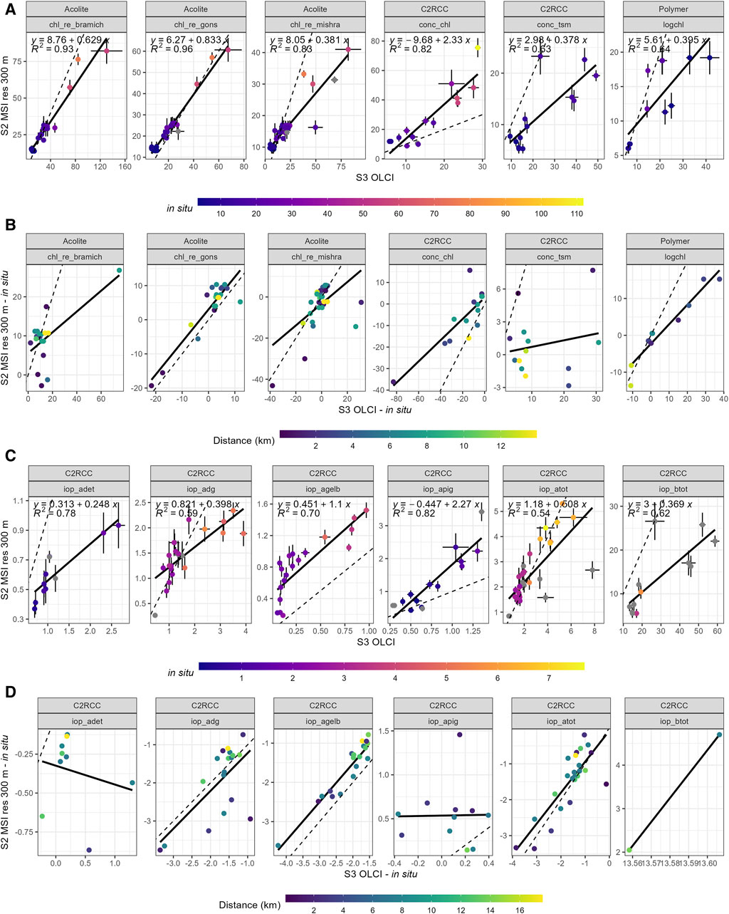
Figure 10. Consistency of S3 OLCI and S2 MSI resampled to 300 m in different in-water algorithms, where row A consists of satellite-derived Chl a (mg/m³) and TSM (mg/L) parameters and row C consists of satellite-derived absorption (m^-1) and scattering (m^-1) parameters. Error bars represent the standard deviation of the 3 × 3 ROI. Gray dots indicate the absence of in situ values. The differences between in situ-measured and satellite-derived OASs and IOPs (B and D) were compared based on the distance from the shore.

The C2RCC in-water algorithms, such as iop_agelb, iop_adet, and iop_apig, showed high correlations between S2 MSI and S3 OLCI (R² > 0.7). However, S2 MSI overestimated the iop_agelb and iop_apig algorithms a_CDOM(443) and a_pig(443) values, respectively, and underestimated the iop_adet algorithm’s a_NAP values compared to S3 OLCI. In situ values of a_CDOM(443) were underestimated by both S2 MSI and S3 OLCI. In situ a_pig(443) values were slightly overestimated by both S2 MSI and S3 OLCI. In situ a_NAP(443) values were underestimated by S2 MSI and overestimated by S3 OLCI. Lower concentration values between S2 MSI and S3 OLCI of the iop_adg (iop_adet + iop_agelb) (<1.5 m^-1), iop_apig (<1 m^-1), and iop_atot (iop_adg + iop_agelb + iop_apig + iop_adet) (<2 m^-1) algorithms aligned well with the 1:1 line. However, higher values resulted in systematic underestimation or overestimation. The sum of all absorption parameters, iop_atot, showed good alignment between S2 MSI and S3 OLCI around the 1:1 line, with a few outliers near the shore. Other C2RCC in-water algorithms (iop_btot, conc_tsm) displayed poor consistency between S2 MSI and S3 OLCI retrievals (R² < 0.65). Some outliers indicated higher spatial variation in the ROI, especially at a distance <5 km. Notable discrepancies were found for the products of conc_chl (C2RCC), iop_adg (C2RCC), iop_apig (C2RCC), iop_atot (C2RCC), iop_btot (C2RCC), and logchl (POLYMER). Differences between satellite data and in situ data were more pronounced near the shore and decreased farther from the shore (>5 km).

4 Discussion

This study compared the performance of 50 satellite-based in-water algorithms. S3 OLCI L2 standard in-water products were validated together with three commonly used alternative processing schemes (ACOLITE, C2RCC, and POLYMER) applied to S3 OLCI and S2 MSI data and a newly developed A4O processing scheme applied to S3 OLCI. The accuracy of these algorithms was assessed using an extensive in situ dataset collected from Estonian lakes and coastal areas, representing eutrophic and absorbing waters. The performance of the in-water algorithms depended on the water type, with systematic underestimation or overestimation in some cases. They were effective for certain ranges of in situ values but not for others. The adjacency effect increased errors near the shore.

4.1 Chl a and TSM in-water algorithms

In this study, in situ Chl a concentrations ranged from 1.5 to 341 mg/m³ (average 24.8 mg/m³), TSM concentrations ranged from 0.005 to 143.3 mg/L (average 9 mg/L), and a_CDOM(442) ranged from 0.4 to 48 m^-1 (average 3.8 m^-1). The high variability made the retrieval of Chl a concentrations from satellite data challenging. S3 OLCI showed the highest accuracy for Chl a retrieval with the chl_re_gons and chl_re_mishra in-water algorithms (ACOLITE), achieving MdPE < −10% and MdAPE ∼24%; data gathered were close to the 1:1 line with a slope of 1.02, an intercept of 2.3, and an R² > 0.58. However, these algorithms are type-dependent. The chl_re_gons algorithm performs poorly for concentrations greater than 40 mg/m³, and the chl_re_mishra algorithm performs poorly for concentrations above 20 mg/m³. Vanhellemont and Ruddick (2021) compared the chl_re_gons in-water algorithm (ACOLITE) applied to different processing schemes over turbid Belgian waters, finding that all processing schemes (POLYMER, ACOLITE, and L2-WFR), except C2RCC, yielded good results (R² > 0.8). The ACOLITE chl_re_gons algorithm performed well (R² > 0.9) due to its similar reflectance spectrum to in situ radiometric measurements, which is related to the assumption of spatially consistent aerosols, making the products less noisy. However, Chl a concentration was slightly overestimated for in situ values above 20 mg/m³. Schaeffer et al. (2022) applied the conc_chl in-water algorithm (C2RCC) to S3 OLCI data over United States lakes, which performed poorly over highly (hyper) eutrophic lakes, recommending its use on waters with Chl a above 20 mg/m³. These results aligned with the current study, where the conc_chl algorithm (C2RCC) performed poorly for Chl a concentrations above 20 mg/m³. For S2 MSI, the chl_re_moses3b and chl_re_moses3b740 algorithms (ACOLITE) performed well for Chl a concentrations above 30 mg/m³. Other in-water algorithms showed high dispersion for concentrations below 20 mg/m³ and systematic overestimation or underestimation for concentrations above 20 mg/m³.

In this study, the average in situ TSM concentration was 9 mg/L, with a maximum match-up value of 143.3 mg/L. The conc_tsm algorithm (C2RCC) and TSM_NN product (L2) performed well in retrieving small TSM concentrations (below 10 mg/L) from S3 OLCI. Higher concentrations were overestimated by all in-water algorithms applied to S3 OLCI data (MdPE > 88%). In contrast, S2 MSI’s in-water algorithms provided TSM concentrations close to the 1:1 line, especially with conc_tsm (C2RCC) (MdAPE = 24%, MdPE = −12%, slope of 0.97, intercept of −0.69, and R² = 0.74), but the accuracy diminished for the in situ values above 15 mg/L. The SPM_Nechad2016_665 algorithm (ACOLITE) performed well for TSM concentrations below 10 mg/L. Generally, band ratio methods (Gons et al. (2002) or Nechad et al. (2010) algorithms of ACOLITE) outperformed NN methods, particularly in waters with high concentrations of scattering material (phytoplankton and TSM) and high Rrs in green-red bands, as ACOLITE in-water algorithms are developed for such waters.

Salama et al. (2022) studied the Ems Dollard estuary (a hyper-turbid waterbody) in the Netherlands, comparing in situ Chl a concentrations with the conc_chl (C2RCC) and Gons model (ACOLITE) (Gons, 1999) and in situ TSM with the Nechad-705 model (ACOLITE) (Nechad et al., 2010) applied to S2 MSI and S3 OLCI data. They found that S2 MSI results had larger errors than S3 OLCI results, with the Gons model for Chl a retrieval having fewer errors than the Nechad model for TSM retrieval. In the current study, the chl_re_gons algorithm had fewer errors for S3 OLCI than for S2 MSI, but S2 MSI had fewer errors with the SPM_Nechad2016_665 algorithm. In conclusion, TSM concentrations retrieved from S2 MSI were accurate, while TSM concentrations retrieved from S3 OLCI were systematically overestimated.

To achieve more accurate results for OAS concentration retrieval, a water-type guided approach could be used, as suggested by Moore et al. (2014); Soomets et al. (2020); Uudeberg et al. (2020). Soomets et al. (2020) examined TSM, Chl a, and a_CDOM(442) retrieval from C2RCC with standard in-water algorithms and band ratio models applied to S2 MSI and S3 OLCI data. Data from four optically different lakes were grouped into five different optical water types introduced by Uudeberg et al. (2019). They found that the conc_tsm algorithm was best suited for moderate and very turbid waters, while band ratio models performed best for other parameters and water types. Soomets et al. (2020) showed that the pre-classification into optical water types improved the performance of in-water algorithms, with correlations close to 0.9.

This study focused on comparing existing commonly used processing schemes applicable to S2 MSI and S3 OLCI data. The A4O approach is based on NN and optical water type classification, while C2RCC is an NN-based processing scheme applied to L1 top-of-atmosphere spectra (entire spectra are taken into processing). When there are high discrepancies in the blue or red part of the spectrum, OAS retrieval performance is poor, which is often the case for Case 2 waters. Further analysis could be conducted by applying band ratio methods, such as the Gons et al. (2002) method, to all AC processors to see how they improve the retrieval of Chl a and TSM concentrations in optically complex waters. This approach is likely to yield better results because specific band reflectance values are more accurate for estimating OAS concentrations.

4.2 IOP in-water algorithms

Rrs depends on the IOPs (Shi et al., 2018), which contribute to bio-optical modeling (Lee et al., 2002; Giardino et al., 2017), including the diffuse attenuation coefficient, TSM, and dissolved and particulate carbon and Chl a concentration retrieval (Kirk, 1981; Lee et al., 2005). However, accurately retrieving these parameters in optically complex waters is challenging.

Previous results indicate that the studied processing schemes struggled to accurately retrieve different absorption products. Among all processing schemes, C2RCC was able to derive more accurate absorption products for S3 OLCI compared to others, although the retrieved values were not always close to the 1:1 line (slope below 0.8 or above 1.3). Both a_CDOM(443) and a_dg(443) were significantly underestimated, as was a_tot(443), showing similar tendencies. Despite this, a_tot(443) was still better estimated (with lower errors) than its individual components.

All processing schemes had difficulties retrieving a_CDOM(443). A low correlation (R² < 0.1), high dispersion (MdAPE > 59%), and strong systematic underestimation (MdPE < −28%) of a_CDOM(443) were observed for both S3 OLCI and S2 MSI across all in-water algorithms. The underestimation of a_CDOM(443) increased for values higher than 1 m^-1. The AC results differ depending on the spectral range. The difficulties of retrieving a_CDOM(443) are due to its strong light absorption and high quantities in the studied waterbodies (e.g., a peak value of 48 m^-1 in Lake Mustjärv). The in-water algorithms are not designed for such high absorption levels; for example, A4O is designed for a maximum a_CDOM(440) of approximately 20 m^-1. This high absorption masks the presence of other products, resulting in a weak signal reflected back to the sensor, making it difficult to capture (Brezonik et al., 2015).

In conclusion, a_tot(443) retrieved from S3 OLCI L1 data was estimated to be the most accurate, but breaking it down into individual components increased the errors. Absorption products derived from S2 MSI L1 data were significantly affected by the adjacency effect, leading to high errors near the shore.

The backscattering coefficient is proportional to the TSM concentration, making it an essential parameter for generating TSM algorithms. However, retrieving scattering in-water products using in-water algorithms for both S2 MSI and S3 OLCI was difficult due to the significant heterogeneity of particles (organic and mineral) in the optically diverse water bodies. The iop_btot algorithm (C2RCC) performed better than iop_bpart (R² = 0.81 and 0.07, respectively), but it still showed a high overestimation (MdPE = 308%). The low performance of iop_bpart could be linked to the calculation methodology of in situ values.

In addition to S3 OLCI L2 products and commonly used processing schemes (C2RCC, ACOLITE, and POLYMER), a recently developed processing scheme, A4O, was studied. A4O was specifically developed for diverse optical water types (Hieronymi et al., 2023). In the current study, the waterbodies were not divided into different water types; instead, the data were analyzed collectively. Among the A4O in-water algorithms, CHL_IOP_ONNS (Chl a) and TSM_ONNS (TSM) provided the most accurate results. Other in-water algorithms had low correlations, high biases, and high dispersion (Figures 2, 4, 5). There were 5–7 times fewer match-ups with A4O than other processing schemes due to the adjacency flag. This was particularly evident for scattering parameters in Figure 7, where there were few match-ups. Although the number of match-ups was not sufficient for comprehensive statistical analysis, they indicated whether there was systematic underestimation or overestimation of the products and their suitability for eutrophic and absorbing waters. In the future, it would be beneficial to test A4O after dividing waterbodies into similar optical water types.

The number of remaining match-ups used for the validation calculated from the total number of match-ups showed the effect of flagging. It was observed that A4O had the fewest match-ups (frequency < 13%), mainly due to three flags, which were raised individually or simultaneously, with the adjacency flag having the highest impact. Approximately 14%–33% of match-ups remained for the C2RCC in-water algorithms, primarily due to the cloud_risk flag, which was raised in over 51% of cases. The Rtosa_OOS and Rhow_OOS flags were raised simultaneously or individually in up to 60% of cases, and the quality_flag_sun_glint_risk flag was raised in 8%–19% of cases. S2 MSI had more match-ups remaining (48%–79%) after flagging than S3 OLCI. ACOLITE provided the most match-ups compared to other AC processors for S2 MSI (61%–79%).

4.3 Accuracy of satellite-derived and in situ data

Generally, the S3 validation protocol recommends using 3 × 3 ROIs, except for very dynamic areas (Concha et al., 2021). In the current study, 3 × 3 ROIs were less sensitive to outliers compared to 1 × 1 ROIs, and their statistical results were generally better.

Multiple statistics were calculated to validate the satellite-derived data. The primary statistical metrics used were MdAPE and MdPE, which are error estimations providing information on the dispersion from the correlation line and bias relative to the 1:1 line. For secondary and visual observations, R², slope, and intercept were used to indicate how well the values derived with in-water algorithms fit the actual values in the linear regression. These statistics should be considered simultaneously to determine which in-water algorithms can be used in eutrophic and absorbing lakes. For example, in the case of the chl_re_moses3b in-water algorithm (ACOLITE) applied to S2 MSI, MdAPE (17%) and MdPE (17%) had low values, indicating low dispersion and bias. However, an R² value of 0.02 showed low correlations, indicating that the performance cannot be considered good. Figure 3 shows that there was very high dispersion for low Chl a concentrations (below 20 mg/m³), increasing the errors close to the shoreline and causing the low R² value. The chl_re_Moses3b algorithm performed well for Chl a concentrations above 30 mg/m³ and for off-shore data. The CHL_ONNS in-water algorithm from the A4O processing scheme had a high R² value (0.67), but the dispersion and bias were also very high (MdAPE and MdPE = 175%), indicating systematic overestimation. Therefore, the algorithms’ performance is poor. In some cases, all statistics showed good consistency, such as for the chl_re_gons algorithm (ACOLITE), where all statistics indicated a good performance (R² = 0.70, MdAPE = 23%, and MdPE = 10%). In reality, these statistics cannot be used as definitive indicators of accuracy for evaluating the actual performance of standard in-water algorithms. In any case, R² should not be prioritized over bias and dispersion.

Certain satellite-derived products were provided with associated uncertainties. Generally, no visible tendencies were observed that could be linked to the proximity of the land or deviation from the 1:1 line. However, uncertainties for the ADG443_NN (L2) product and the iop_atot, iop_adg, and iop_agelb algorithms (C2RCC) derived from S3 OLCI were higher specifically for outliers that clearly overestimated the in situ measured values. The Sentinel 3 mission requirements document (Drinkwater and Rebhan, 2007) provides thresholds that should not be exceeded to achieve an acceptable accuracy of the parameters for the S3 OLCI sensor in optically complex waters. The accuracy threshold for Chl a, TSM concentrations, and a_CDOM(412) is 70%, but the goal is to achieve 10%. To estimate the accuracy of the S3 OLCI products, uncertainties should be estimated for both satellite-derived and in situ-measured OASs and IOPs. Accurate uncertainty budgets have been estimated for radiometric data (Alikas et al., 2020; Banks et al., 2020; Lin et al., 2022) but not for OAS concentrations and IOPs. Therefore, calculating the correct uncertainties for each satellite-derived product and in situ data is needed in the future.

4.4 Errors associated with the vicinity of the land

To estimate errors associated with the vicinity of the land, Chl a match-ups were analyzed in relation to the distance from the shore. Higher errors appeared closer to the shore (<5 km) and decreased further away from shore due to the adjacency effect on the pixels near land (Kiselev et al., 2015; Warren et al., 2019a; Paulino et al., 2022). S2 MSI algorithms had a higher overall error (∼280%) between distance groups close to the shore (<5 km) and away from the shore (>5 km) than S3 OLCI (∼70%). This could be linked to the difference in spatial resolution, where the S2 MSI pixel size (10 m) is 30 times smaller than the S3 OLCI pixel size (300 m). Steinmetz and Ramon (2018) stated that POLYMER is robust near land, which is explained by the model’s consideration of aerosol signals and non-water components (e.g., adjacency effect). Our study shows that the POLYMER Chl a in-water algorithm had low errors (APE < 100%) both close to and away from the shore for S2 MSI and S3 OLCI, with a mean error difference of only ∼30%. Similar results were found by Alikas et al. (2020), where POLYMER was least influenced by the adjacency effect based on S3 OLCI reflectance data. S2 MSI ACOLITE Chl a algorithms exhibited high errors near the shore, potentially due to higher reflectance values in the red and NIR bands, as reported by Martins et al. (2017) and Renosh et al. (2020). Several studies have estimated the adjacency effect on satellite data, this effect on pixels farther than 10 km from the shore (Beltrán-Abaunza et al., 2014), and even up to 40 km (Bulgarelli et al., 2014; Bulgarelli and Zibordi, 2018a). Bulgarelli and Zibordi (2018a) compared S2 MSI and S3 OLCI reflectance data, finding an adjacency effect up to ∼36 km from the shore for S3 OLCI and ∼20 km for S2 MSI. However, these studies focus on seas and oceans, not lakes. These results indicate that the errors between satellite retrievals and in situ measurements tend to be higher in the vicinity of the land, pointing to the need for adjacency correction and additional research on this topic.

4.5 S2 MSI vs. S3 OLCI

In-water algorithms applied to S3 OLCI and S2 MSI resampled data were compared to assess the consistency between the sensors’ outputs for combining data in further studies. Among the 50 in-water algorithms evaluated, 12 similar algorithms could be applied to both satellites, with Chl a algorithms comprising the majority (5 out of 12). The chl_re_gons algorithm (ACOLITE) showed high consistency (slope of 0.8, R² = 0.96, close to 1:1 line); however, Chl concentrations below 20 mg/m³ were slightly overestimated by S2 MSI data. It means that S2 MSI and S3 OLCI-derived time series will differ in specific Chl a ranges, even when a similar algorithm is applied. Other ACOLITE Chl a in-water algorithms, chl_re_bramich and chl_re_mishra, also had high correlations (R² > 0.8), whereas Chl a concentrations above 20 mg/m³ were underestimated by S2 MSI data. Cazzaniga et al. (2019) compared S2 MSI and S3 OLCI data over two large Italian lakes using the Bio-Optical Model-Based tool for Estimating water quality and bottom properties from Remote sensing images (BOMBER) and found a good correlation between S2 MSI and S3 OLCI data (R² > 0.8). Their study showed overestimation by S2 MSI for Chl a concentrations below 1.5 mg/m³ in Lake Garda. However, the study found that S2 MSI could capture higher concentrations with smaller variations than S3 OLCI in Lake Trasimeno, where Chl a concentrations reached up to 100 mg/m³. In our study, other in-water algorithms showed low consistency, which could be attributed to the different characteristics of the sensors, such as spectral and radiometric resolution. Outliers were more common further from the shore (>5 km), where greater spatial variability within 3 × 3 ROIs was apparent. Although only a few studies have compared the S2 MSI and S3 OLCI data, many studies have shown the integration between the S2 MSI and S3 OLCI (Sòria-Perpinyà et al., 2021; Salama et al., 2022). The combination of both satellites could provide more frequent data, with S2 MSI offering higher spatial resolution to complement S3 OLCI data.

5 Conclusion

The water quality of optically complex eutrophic and absorbing lakes is influenced by various OASs and their IOPs. These OASs and their IOPs can be derived from satellite data, such as Copernicus S2 MSI and S3 OLCI, using in-water algorithms to support the monitoring of these ecosystems. These algorithms are designed for water applications to derive water quality products, including Chl a and TSM concentrations, the absorption of CDOM, phytoplankton, non-algal particles, and their combinations, as well as scattering. All these are important inputs for different models.

This study demonstrated that the S3 OLCI chl_re_gons (ACOLITE) and S2 MSI conc_tsm (C2RCC) algorithms’ retrievals were the most accurate, with low dispersion and biases (MdAPE = 23% and 24% and MdPE = 10% and −12%, respectively). Total absorption was retrieved more accurately than its components, with a_CDOM(443) and a_dg(443) contributing the most. The results from 3 × 3 ROIs were almost always better than those from 1 × 1 pixel data. The study showed a decrease in errors (APE < 100%) between satellite-derived and in situ-measured Chl a further away from the shore (>5 km). The mean errors were higher in the distance group close to the shore (<5 km) (S2 MSI 315% and S3 OLCI 150%) and lower off the shore (>5 km) (S2 MSI 35% and S3 OLCI 80%). The POLYMER Chl a in-water algorithms (logchl) showed lower errors (<100%) even close to the shore for both S2 MSI and S3 OLCI, with a low and consistent difference in both distance groups (30%). For estimating the consistency between the S2 MSI and S3 OLCI in-water algorithms, chl_re_gons (ACOLITE) showed high consistency between both satellites, close to a 1:1 line with R² = 0.96. However, Chl a concentrations below 20 mg/m³ were overestimated by S2 MSI data.

The study indicates a need for further development of in-water algorithms, especially for high-absorbing and eutrophic waters. We also indirectly showed the strong dependence of the algorithms on upstream atmospheric correction, particularly for NN-based algorithms that use almost the entire reflectance spectrum as input. Algorithms based on fewer bands, preferably in the central visible range, could offer advantages. Priority should be given to more reliable discrimination of the optical effects of the water constituents and a system-adjustment of atmospheric correction and in-water algorithms. For more precise estimation and identification of the best in-water algorithms, the classification of optically complex waters should be considered in further studies. Additionally, influences related to the vicinity of the land in lakes and, in particular, the compatibility between S2 MSI and S3 OLCI should be investigated. Corresponding adjacency warnings and other flags are evaluated very differently in the algorithms and are sometimes not recognized, which is reflected in the number of match-ups. Accordingly, the handling of flags should be better defined and generalized in matchup analyses, i.e., through a common best-quality approach. Based on this study, further investigation is essential for improving the accuracy and reliability of in-water algorithms.

Data availability statement

The raw data supporting the conclusions of this article will be made available by the authors, without undue reservation.

Author contributions

AA-T: conceptualization, data curation, formal analysis, investigation, methodology, software, validation, visualization, writing–original draft, and writing–review and editing. MU: conceptualization, data curation, formal analysis, investigation, methodology, software, validation, writing–original draft, and writing–review and editing. KK: data curation, funding acquisition, resources, and writing–review and editing. MH: data curation, writing–review and editing, and formal analysis. KA: conceptualization, funding acquisition, methodology, project administration, resources, writing–review and editing, data curation, formal analysis, investigation, and supervision.

Funding

The author(s) declare that financial support was received for the research, authorship, and/or publication of this article. This research was funded by the 1) European Commission grant named “Framework Partnership Agreement on Copernicus User Uptake” (MLTTO18557); 2) Estonian Research Council personal starting grant PSG10; 3) Estonian Research Council group grant PRG302; and 4) European Union’s Horizon Europe research and innovation programme grant named SpongeBoost (101112906).

Acknowledgments

The authors would like to thank people from the Centre for Limnology, Estonian University of Life Sciences, and the water remote sensing work group from Tartu Observatory, University of Tartu, for collecting and providing in situ water quality data. They would like to thank the Department of Remote Sensing and Marine Optics, Estonian Marine Institute, University of Tartu, for providing WET Labs instruments. The authors also thank the two reviewers for their valuable contribution.

Conflict of interest

The authors declare that the research was conducted in the absence of any commercial or financial relationships that could be construed as a potential conflict of interest.

Publisher’s note

All claims expressed in this article are solely those of the authors and do not necessarily represent those of their affiliated organizations, or those of the publisher, the editors, and the reviewers. Any product that may be evaluated in this article, or claim that may be made by its manufacturer, is not guaranteed or endorsed by the publisher.

Supplementary material

The Supplementary Material for this article can be found online at: https://www.frontiersin.org/articles/10.3389/frsen.2024.1423332/full#supplementary-material

References

Alikas, K., Ansko, I., Vabson, V., Ansper, A., Kangro, K., Uudeberg, K., et al. (2020). Consistency of radiometric satellite data over lakes and coastal waters with local field measurements. Remote Sens. 12, 616. doi:10.3390/rs12040616

CrossRef Full Text | Google Scholar

Ansper, A., and Alikas, K. (2019). Retrieval of chlorophyll a from sentinel-2 MSI data for the European union water framework directive reporting purposes. Remote Sens. 11, 64. doi:10.3390/rs11010064

CrossRef Full Text | Google Scholar

Baker, E. T., and Lavelle, J. W. (1984). The effect of particle size on the light attenuation coefficient of natural suspensions. JGR Ocean. 89, 8197–8203. doi:10.1029/JC089iC05p08197

CrossRef Full Text | Google Scholar

Banks, A. C., Vendt, R., Alikas, K., Bialek, A., Kuusk, J., Lerebourg, C., et al. (2020). Fiducial reference measurements for satellite ocean colour (FRM4SOC). Remote Sens. 12, 1322. doi:10.3390/RS12081322

CrossRef Full Text | Google Scholar

Beltrán-Abaunza, J. M., Kratzer, S., and Brockmann, C. (2014). Evaluation of MERIS products from Baltic Sea coastal waters rich in CDOM. Ocean. Sci. 10, 377–396. doi:10.5194/os-10-377-2014

CrossRef Full Text | Google Scholar

Bhangale, U., More, S., Shaikh, T., Patil, S., and More, N. (2020). Analysis of surface water resources using sentinel-2 imagery. Procedia Comput. Sci. 171, 2645–2654. doi:10.1016/j.procs.2020.04.287

CrossRef Full Text | Google Scholar

Bourrin, F., Uusõue, M., Artigas, M. C., Sànchez-Vidal, A., Aubert, D., Menniti, C., et al. (2021). Release of particles and metals into seawater following sediment resuspension of a coastal mine tailings disposal off Portmán Bay, Southern Spain. Environ. Sci. Pollut. Res. 28, 47973–47990. doi:10.1007/s11356-021-14006-1

CrossRef Full Text | Google Scholar

Bramich, J., Bolch, C. J. S., and Fischer, A. (2021). Improved red-edge chlorophyll-a detection for Sentinel 2. Ecol. Indic. 120, 106876. doi:10.1016/j.ecolind.2020.106876

CrossRef Full Text | Google Scholar

Brezonik, P. L., Olmanson, L. G., Finlay, J. C., and Bauer, M. E. (2015). Factors affecting the measurement of CDOM by remote sensing of optically complex inland waters. Remote Sens. Environ. 157, 199–215. doi:10.1016/j.rse.2014.04.033

CrossRef Full Text | Google Scholar

Brockmann, C., Doerffer, R., Peters, M., Stelzer, K., Embacher, S., and Ruescas, A. (2016). Evolution of the C2RCC neural network for sentinel 2 and 3 for the retrieval of ocean colour products in normal and extreme optically complex waters. 7823–7830.

Google Scholar

Bulgarelli, B., Kiselev, V., and Zibordi, G. (2014). Simulation and analysis of adjacency effects in coastal waters: a case study. Appl. Opt. 53, 1523. doi:10.1364/ao.53.001523

PubMed Abstract | CrossRef Full Text | Google Scholar

Bulgarelli, B., and Zibordi, G. (2018a). Analysis of adjacency effects for Copernicus ocean colour missions. doi:10.2760/178467

CrossRef Full Text | Google Scholar

Bulgarelli, B., and Zibordi, G. (2018b). On the detectability of adjacency effects in ocean color remote sensing of mid-latitude coastal environments by SeaWiFS, MODIS-A, MERIS, OLCI, OLI and MSI. Remote Sens. Environ. 209, 423–438. doi:10.1016/j.rse.2017.12.021

PubMed Abstract | CrossRef Full Text | Google Scholar

Burd, A. B., and Jackson, G. A. (2009). Particle aggregation. Ann. Rev. Mar. Sci. 1, 65–90. doi:10.1146/annurev.marine.010908.163904

PubMed Abstract | CrossRef Full Text | Google Scholar

Cazzaniga, I., Bresciani, M., Colombo, R., Della Bella, V., Padula, R., and Giardino, C. (2019). A comparison of Sentinel-3-OLCI and Sentinel-2-MSI-derived Chlorophyll-a maps for two large Italian lakes. Remote Sens. Lett. 10, 978–987. doi:10.1080/2150704X.2019.1634298

CrossRef Full Text | Google Scholar

Coble, P. G. (2007). Marine optical biogeochemistry: the chemistry of ocean color. Chem. Rev. 107, 402–418. doi:10.1021/cr050350+

PubMed Abstract | CrossRef Full Text | Google Scholar

Concha, J. A., Bracaglia, M., and Brando, V. E. (2021). Assessing the influence of different validation protocols on Ocean Colour match-up analyses. Remote Sens. Environ. 259, 112415. doi:10.1016/j.rse.2021.112415

CrossRef Full Text | Google Scholar

Doerffer, R., and Schiller, H. (2007). The MERIS case 2 water algorithm. Int. J. Remote Sens. 28, 517–535. doi:10.1080/01431160600821127

CrossRef Full Text | Google Scholar

Downing, J. A. (2014). “Productivity of freswater ecosystems and climate change,” in Global environmental change (Netherlands: Springer Netherlands), 221–229. doi:10.1007/978-94-007-5784-4_127

CrossRef Full Text | Google Scholar

Drinkwater, M., and Rebhan, H. (2007). Sentinel-3: mission requirements document. EOP-SMO/1151/MD-md.

Google Scholar

Du, Y., Zhang, Y., Ling, F., Wang, Q., Li, W., and Li, X. (2016). Water bodies’ mapping from Sentinel-2 imagery with Modified Normalized Difference Water Index at 10-m spatial resolution produced by sharpening the swir band. Remote Sens. 8, 354. doi:10.3390/rs8040354

CrossRef Full Text | Google Scholar

Duckey, T., Lewis, M., and Chang, G. (2006). Optical oceanography: recent advances and future directions using global remote sensing and in situ observations. Rev. Geophys. 44, 1–39. doi:10.1029/2003RG000148

CrossRef Full Text | Google Scholar

Dyer, K. R., Christie, M. C., Feates, N., Fennessy, M. J., Pejrup, M., and Van Der Lee, W. (2000). An investigation into processes influencing the morphodynamics of an intertidal mudflat, the Dollard Estuary, The Netherlands: I. Hydrodynamics and suspended sediment. Estuar. Coast. Shelf Sci. 50, 607–625. doi:10.1006/ecss.1999.0596

CrossRef Full Text | Google Scholar

ESA (2016). Sentinel-3 family grows. Available at: https://www.esa.int/Applications/Observing_the_Earth/Copernicus/Sentinel-3/Sentinel-3_family_grows (Accessed April 1, 2024).

Google Scholar

ESA (2021). Gearing up for third Sentinel-2 satellite. Available at: https://www.esa.int/Applications/Observing_the_Earth/Copernicus/Sentinel-2/Gearing_up_for_third_Sentinel-2_satellite (Accessed April 1, 2024).

Google Scholar

ESS (1993). ESS Method 340.2. Total suspended solids, mass balance (dried at 103-105^o C), volatile suspended solids (Ignited at 550^o C). Environ. Sci. Sect., 189–192. Available at: http://www.cyanopros.com/refs/epa_TSS.pdf (Accessed February 1, 2019).

Google Scholar

EUMETSAT (2021a). Recommendations for sentinel-3 OLCI ocean Colour product validations in comparison with in situ measurements – matchup protocols. USA: EUM/SEN3/D.

Google Scholar

EUMETSAT (2021b). Sentinel-3 OLCI L2 report for baseline collection OL_L2M_003. EUM/RSP/REP/21/1211386 v2B.

Google Scholar

EUMETSAT (2024). No title. Available at: https://user.eumetsat.int/resources/user-guides/sentinel-3-ocean-colour-level-2-data-guide.

Google Scholar

Giardino, C., Bresciani, M., Braga, F., Cazzaniga, I., De Keukelaere, L., Knaeps, E., et al. (2017). Bio-optical modeling of total suspended solids. Elsevier Inc. doi:10.1016/B978-0-12-804644-9.00005-7

CrossRef Full Text | Google Scholar

Giardino, C., Kõks, K.-L., Bolpagni, R., Luciani, G., Candiani, G., Lehmann, M. K., et al. (2019). “The color of water from space: a case study for Italian lakes from sentinel-2,” in Geospatial analyses of earth observation (EO) data (China: IntechOpen). Available at: https://www.intechopen.com/chapters/67603.

CrossRef Full Text | Google Scholar

Gons, H. J. (1999). Optical teledetection of chlorophyll a in turbid inland waters. Environ. Sci. Technol. 33, 1127–1132. doi:10.1021/es9809657

CrossRef Full Text | Google Scholar

Gons, H. J., Rijkeboer, M., and Ruddick, K. G. (2002). A chlorophyll-retrieval algorithm for satellite imagery (Medium Resolution Imaging Spectrometer) of inland and coastal waters. J. Plankton Res. 24, 947–951. doi:10.1093/plankt/24.9.947

CrossRef Full Text | Google Scholar

Grendaitė, D., Stonevičius, E., Karosienė, J., Savadova, K., and Kasperovičienė, J. (2018). Chlorophyll-a concentration retrieval in eutrophic lakes in Lithuania from Sentinel-2 data. Geol. Geogr. 4, 15–28. doi:10.6001/geol-geogr.v4i1.3720

CrossRef Full Text | Google Scholar

Hieronymi, M. (2019). Spectral band adaptation of ocean color sensors for applicability of the multi-water biogeo-optical algorithm ONNS. Opt. Express 27, A707. doi:10.1364/oe.27.00a707

PubMed Abstract | CrossRef Full Text | Google Scholar

Hieronymi, M., Bi, S., Müller, D., Schütt, E. M., Behr, D., Brockmann, C., et al. (2023). Ocean color atmospheric correction methods in view of usability for different optical water types. Front. Mar. Sci. 10, 1–23. doi:10.3389/fmars.2023.1129876

CrossRef Full Text | Google Scholar

Hieronymi, M., Müller, D., and Doerffer, R. (2017). The OLCI neural network swarm (ONNS): a bio-geo-optical algorithm for open ocean and coastal waters. Front. Mar. Sci. 4. doi:10.3389/fmars.2017.00140

CrossRef Full Text | Google Scholar

Huisman, J., Codd, G. A., Paerl, H. W., Ibelings, B. W., Verspagen, J. M. H., and Visser, P. M. (2018). Cyanobacterial blooms. Nat. Rev. Microbiol. 16, 471–483. doi:10.1038/s41579-018-0040-1

PubMed Abstract | CrossRef Full Text | Google Scholar

Istvánovics, V. (2009). Eutrophication of lakes and reservoirs. Encycl. Inl. Waters, 157–165. doi:10.1016/B978-012370626-3.00141-1

CrossRef Full Text | Google Scholar

Jeffrey, S. W., and Humphrey, G. F. (1975). New spectrophotometric equations for determining chlorophylls a, b, c1 and c2 in higher plants, algae and natural phytoplankton. Biochem. Physiol. Pflanz. 167, 191–194. doi:10.1016/S0015-3796(17)30778-3

CrossRef Full Text | Google Scholar

Kapanen, G. (2018). Lake Peipsi as a biggest transboundary lake in Europe. Dynamiques environnementales 42, 398–409. doi:10.4000/dynenviron.2680

CrossRef Full Text | Google Scholar

Kasprzak, P., Padisák, J., Koschel, R., Krienitz, L., and Gervais, F. (2008). Chlorophyll a concentration across a trophic gradient of lakes: an estimator of phytoplankton biomass? Limnologica 38, 327–338. doi:10.1016/j.limno.2008.07.002

CrossRef Full Text | Google Scholar

Keskkonnaagentuur (2024). EELIS. Available at: https://infoleht.keskkonnainfo.ee/.

Google Scholar

Kirk, J. (2011). Light and photosynthesis in aquatic ecosystems. Cambridge: Cambridge University Press.

Google Scholar

Kirk, J. T. (1981). Monte Carlo study of the nature of the underwater light field in, and the relationships between optical properties of, turbid yellow waters. Mar. Freshw. Res. 32, 517–532. doi:10.1071/MF9810517

CrossRef Full Text | Google Scholar

Kiselev, V., Bulgarelli, B., and Heege, T. (2015). Sensor independent adjacency correction algorithm for coastal and inland water systems. Remote Sens. Environ. 157, 85–95. doi:10.1016/j.rse.2014.07.025

CrossRef Full Text | Google Scholar

Kyryliuk, D., and Kratzer, S. (2019). Summer distribution of total suspended matter across the Baltic Sea. Front. Mar. Sci. 5, 1–16. doi:10.3389/fmars.2018.00504

CrossRef Full Text | Google Scholar

Lee, Z., Carder, K. L., and Arnone, R. A. (2002). Deriving inherent optical properties from water color: a multiband quasi-analytical algorithm for optically deep waters. Appl. Opt. 41, 5755. doi:10.1364/ao.41.005755

PubMed Abstract | CrossRef Full Text | Google Scholar

Lee, Z. P., Du, K. P., and Arnone, R. (2005). A model for the diffuse attenuation coefficient of downwelling irradiance. J. Geophys. Res. Ocean. 110, 1–10. doi:10.1029/2004JC002275

CrossRef Full Text | Google Scholar

Lin, J., Dall’Olmo, G., Tilstone, G. H., Brewin, R. J. W., Vabson, V., Ansko, I., et al. (2022). Derivation of uncertainty budgets for continuous above-water radiometric measurements along an Atlantic Meridional Transect. Opt. Express 30, 45648. doi:10.1364/oe.470994

PubMed Abstract | CrossRef Full Text | Google Scholar

Marra, J., Trees, C. C., and O’Reilly, J. E. (2007). Phytoplankton pigment absorption: a strong predictor of primary productivity in the surface ocean. Deep. Res. Part I Oceanogr. Res. Pap. 54, 155–163. doi:10.1016/j.dsr.2006.12.001

CrossRef Full Text | Google Scholar

Martins, V. S., Barbosa, C. C. F., de Carvalho, L. A. S., Jorge, D. S. F., Lobo, F. de L., and de Moraes Novo, E. M. L. (2017). Assessment of atmospheric correction methods for sentinel-2 MSI images applied to Amazon floodplain lakes. Remote Sens. 9, 322. doi:10.3390/rs9040322

CrossRef Full Text | Google Scholar

Mishra, S., and Mishra, D. R. (2012). Normalized difference chlorophyll index: a novel model for remote estimation of chlorophyll-a concentration in turbid productive waters. Remote Sens. Environ. 117, 394–406. doi:10.1016/j.rse.2011.10.016

CrossRef Full Text | Google Scholar

Mobley, C. D. (1994). “Optical properties of water,” in Light and water: radiative transfer in natural waters (Germany: Academic Press), 60–142.

Google Scholar

Mobley, C. D. (2022). “Optical constituents of the ocean,” in The oceanic optics book. Editors C. D. Mobley, and N. S. Darthmouth (Canada: International Ocean Colour Coordinating Group IOCCG), 924. doi:10.25607/OBP-1710

CrossRef Full Text | Google Scholar

Mograne, M. A., Jamet, C., Loisel, H., Vantrepotte, V., Mériaux, X., and Cauvin, A. (2019). Evaluation of five atmospheric correction algorithms over French optically-complex waters for the sentinel-3A OLCI ocean color sensor. Remote Sens. 11, 668–725. doi:10.3390/RS11060668

CrossRef Full Text | Google Scholar

Moore, T. S., Dowell, M. D., Bradt, S., and Ruiz Verdu, A. (2014). An optical water type framework for selecting and blending retrievals from bio-optical algorithms in lakes and coastal waters. Remote Sens. Environ. 143, 97–111. doi:10.1016/j.rse.2013.11.021

PubMed Abstract | CrossRef Full Text | Google Scholar

Morel, A. (1988). Optical modeling of the upper ocean in relation to its biogenous matter content (case I waters). J. Geophys. Res. Ocean. 93, 10749–10768. doi:10.1029/jc093ic09p10749

CrossRef Full Text | Google Scholar

Morel, A., Antoine, D., and Gentili, B. (2002). Bidirectional reflectance of oceanic waters: accounting for Raman emission and varying particle scattering phase function. Appl. Opt. 41, 6289. doi:10.1364/ao.41.006289

PubMed Abstract | CrossRef Full Text | Google Scholar

Morel, A., and Prieur, L. (1977). Analysis of variations in ocean color. Limnol. Oceanogr. 22, 709–722. doi:10.4319/lo.1977.22.4.0709

CrossRef Full Text | Google Scholar

Moses, W. J., Gitelson, A. A., Berdnikov, S., Saprygin, V., and Povazhnyi, V. (2012). Operational MERIS-based NIR-red algorithms for estimating chlorophyll-a concentrations in coastal waters - the Azov Sea case study. Remote Sens. Environ. 121, 118–124. doi:10.1016/j.rse.2012.01.024

CrossRef Full Text | Google Scholar

Nechad, B., Ruddick, K. G., and Neukermans, G. (2009). Calibration and validation of a generic multisensor algorithm for mapping of turbidity in coastal waters. Remote Sens. Ocean. Sea Ice, Large Water Reg. 2009 7473, 74730H. doi:10.1117/12.830700

CrossRef Full Text | Google Scholar

Nechad, B., Ruddick, K. G., and Park, Y. (2010). Calibration and validation of a generic multisensor algorithm for mapping of total suspended matter in turbid waters. Remote Sens. Environ. 114, 854–866. doi:10.1016/j.rse.2009.11.022

CrossRef Full Text | Google Scholar

Nõges, P., and Nõges, T. (2012). “Võrtsjärv Lake in Estonia, in Encyclopedia of Lakes and reservoirs,” in Encyclopedia of earth Sciences series (Dordrecht: Springer), 850–861. doi:10.1007/978-1-4020-4410-6_228

CrossRef Full Text | Google Scholar

Osburn, C. L., Boyd, T. J., Montgomery, M. T., Bianchi, T. S., Coffin, R. B., and Paerl, H. W. (2016). Optical proxies for terrestrial dissolved organic matter in estuaries and coastal waters. Front. Mar. Sci. 2. doi:10.3389/fmars.2015.00127

CrossRef Full Text | Google Scholar

Paavel, B., Arst, H., Metsamaa, L., Toming, K., and Reinart, A. (2011). Optical investigations of CDOM-rich coastal waters in Pärnu Bay. Est. J. Earth Sci. 60, 102–112. doi:10.3176/earth.2011.2.04

CrossRef Full Text | Google Scholar

Pahlevan, N., Mangin, A., Balasubramanian, S. V., Smith, B., Alikas, K., Arai, K., et al. (2021). ACIX-Aqua: a global assessment of atmospheric correction methods for Landsat-8 and Sentinel-2 over lakes, rivers, and coastal waters. Remote Sens. Environ. 258, 112366. doi:10.1016/j.rse.2021.112366

CrossRef Full Text | Google Scholar

Pannard, A., Bormans, M., Lefebvre, S., Claquin, P., and Lagadeuc, Y. (2007). Phytoplankton size distribution and community structure: influence of nutrient input and sedimentary loss. J. Plankton Res. 29, 583–598. doi:10.1093/plankt/fbm040

CrossRef Full Text | Google Scholar

Paulino, R. S., Martins, V. S., Novo, E. M. L. M., Barbosa, C. C. F., de Carvalho, L. A. S., and Begliomini, F. N. (2022). Assessment of adjacency correction over inland waters using sentinel-2 MSI images. Remote Sens. 14, 1829. doi:10.3390/rs14081829

CrossRef Full Text | Google Scholar

Pirasteh, S., Mollaee, S., Fatholahi, S. N., and Li, J. (2020). Estimation of phytoplankton chlorophyll-a concentrations in the western basin of Lake erie using sentinel-2 and sentinel-3 data. Can. J. Remote Sens. 46, 585–602. doi:10.1080/07038992.2020.1823825

CrossRef Full Text | Google Scholar

Renosh, P. R., Doxaran, D., De Keukelaere, L., and Gossn, J. I. (2020). Evaluation of atmospheric correction algorithms for sentinel-2-MSI and sentinel-3-OLCI in highly turbid estuarine waters. Remote Sens. 12, 1285. doi:10.3390/RS12081285

CrossRef Full Text | Google Scholar

Reynolds, R. A., Stramski, D., and Neukermans, G. (2016). Optical backscattering by particles in Arctic seawater and relationships to particle mass concentration, size distribution, and bulk composition. Limnol. Oceanogr. 61, 1869–1890. doi:10.1002/lno.10341

CrossRef Full Text | Google Scholar

Röttgers, R., Bi, S., Burmester, H., Heymann, K., Hieronymi, M., Krasemann, H., et al. (2023). Water inherent optical properties and concentrations of water constituents from the German Bight and adjacent regions. PANGAEA. [dataset bundled publication]. doi:10.1594/PANGAEA.950774

CrossRef Full Text | Google Scholar

Salama, M. S., Spaias, L., Poser, K., Peters, S., and Laanen, M. (2022). Validation of sentinel-2 (MSI) and sentinel-3 (OLCI) water quality products in turbid estuaries using fixed monitoring stations. Front. Remote Sens. 2, 1–17. doi:10.3389/frsen.2021.808287

CrossRef Full Text | Google Scholar

Schaeffer, B., Salls, W., Coffer, M., Lebreton, C., Werther, M., Stelzer, K., et al. (2022). Merging of the Case 2 Regional Coast Colour and Maximum-Peak Height chlorophyll-a algorithms: validation and demonstration of satellite-derived retrievals across US lakes. Environ. Monit. Assess. 194, 179. doi:10.1007/s10661-021-09684-w

PubMed Abstract | CrossRef Full Text | Google Scholar

Schaeffer, B. A., Schaeffer, K. G., Keith, D., Lunetta, R. S., Conmy, R., and Gould, R. W. (2013). Barriers to adopting satellite remote sensing for water quality management. Int. J. Remote Sens. 34, 7534–7544. doi:10.1080/01431161.2013.823524

CrossRef Full Text | Google Scholar

Sent, G., Biguino, B., Favareto, L., Cruz, J., Sá, C., Dogliotti, A. I., et al. (2021). Deriving water quality parameters using sentinel-2 imagery: a case study in the Sado Estuary, Portugal. Remote Sens. 13, 1043–1130. doi:10.3390/rs13051043

CrossRef Full Text | Google Scholar

Shi, W., Zhang, Y., and Wang, M. (2018). Deriving total suspended matter concentration from the near-infrared-based inherent optical properties over turbid waters: a case study in Lake Taihu. Remote Sens. 10, 333–417. doi:10.3390/rs10020333

CrossRef Full Text | Google Scholar

Snyder, W. A., Arnone, R. A., Davis, C. O., Goode, W., Gould, R. W., Ladner, S., et al. (2008). Optical scattering and backscattering by organic and inorganic particulates in U.S. coastal waters. Appl. Opt. 47, 666–677. doi:10.1364/AO.47.000666

PubMed Abstract | CrossRef Full Text | Google Scholar

Soomets, T., Uudeberg, K., Jakovels, D., Brauns, A., Zagars, M., and Kutser, T. (2020). Validation and comparison of water quality products in Baltic Lakes using Sentinel-2 MSI and Sentinel-3 OLCI data. Sensors 3 (2), 742. doi:10.3390/s20030742

PubMed Abstract | CrossRef Full Text | Google Scholar

Sòria-Perpinyà, X., Vicente, E., Urrego, P., Pereira-Sandoval, M., Tenjo, C., Ruíz-Verdú, A., et al. (2021). Validation of water quality monitoring algorithms for sentinel-2 and sentinel-3 in mediterranean inland waters with in situ reflectance data. WaterSwitzerl. 13, 686. doi:10.3390/w13050686

CrossRef Full Text | Google Scholar

Steinmetz, F., Deschamps, P.-Y., and Ramon, D. (2011). Atmospheric correction in presence of sun glint: application to MERIS. Opt. Express 19, 9783. doi:10.1364/oe.19.009783

PubMed Abstract | CrossRef Full Text | Google Scholar

Steinmetz, F., and Ramon, D. (2018). Sentinel-2 MSI and Sentinel-3 OLCI consistent ocean colour products using. POLYMER 13. doi:10.1117/12.2500232

CrossRef Full Text | Google Scholar

Tassan, S., and Ferrari, G. M. (1995). An alternative approach to absorption measurements of aquatic particles retained on filters. Limnol. Oceanogr. 40, 1358–1368. doi:10.4319/lo.1995.40.8.1358

CrossRef Full Text | Google Scholar

The International Organization for Standardization (1992). ISO 10260:1992Water quality—measurement of biochemical parameters—spectrometric determination of the chlorophyll-a concentration. Geneva, Switzerland: ISO.

Google Scholar

The International Organization for Standardization (2018). ISO 5667-3:2018 water quality—sampling—Part 3: preservation and handling of water samples. Geneva, Switzerland: ISO.

Google Scholar

Toming, K., Kutser, T., Laas, A., Sepp, M., Paavel, B., and N�ges, T. (2016). First experiences in mapping lakewater quality parameters with sentinel-2 MSI imagery. Remote Sens. 8, 640–714. doi:10.3390/rs8080640

CrossRef Full Text | Google Scholar

Tzortziou, M., Zeri, C., Dimitriou, E., Ding, Y., Jaffe, R., Anagnostou, E., et al. (2015). Colored dissolved organic matter dynamics and anthropogenic influences in a major transboundary river and its coastal wetland. Limnol. Oceanogr. 60, 1222–1240. doi:10.1002/lno.10092

PubMed Abstract | CrossRef Full Text | Google Scholar

Uudeberg, K., Aavaste, A., Kõks, K. L., Ansper, A., Uusõue, M., Kangro, K., et al. (2020). Optical water type guided approach to estimate optical water quality parameters. Remote Sens. 12, 931–1012. doi:10.3390/RS12060931

CrossRef Full Text | Google Scholar

Uudeberg, K., Ansko, I., Getter, P., and Ansper, A. (2019). Using optical water types to monitor changes in optically complex inland and coastal waters. Remote Sens. 11 (19), 1–20. doi:10.3390/rs11192297

CrossRef Full Text | Google Scholar

Uusõue, M., Ligi, M., Kutser, T., Bourrin, F., Uudeberg, K., Kangro, K., et al. (2022). Effects of different conditions on particle dynamics and properties in West-Estonian coastal areas. Oceanologia 64, 694–716. doi:10.1016/j.oceano.2022.06.006

CrossRef Full Text | Google Scholar

Vanhellemont, Q. (2019). Adaptation of the dark spectrum fitting atmospheric correction for aquatic applications of the Landsat and Sentinel-2 archives. Remote Sens. Environ. 225, 175–192. doi:10.1016/j.rse.2019.03.010

CrossRef Full Text | Google Scholar

Vanhellemont, Q., and Ruddick, K. (2018). Atmospheric correction of metre-scale optical satellite data for inland and coastal water applications. Remote Sens. Environ. 216, 586–597. doi:10.1016/j.rse.2018.07.015

CrossRef Full Text | Google Scholar

Vanhellemont, Q., and Ruddick, K. (2021). Atmospheric correction of Sentinel-3/OLCI data for mapping of suspended particulate matter and chlorophyll-a concentration in Belgian turbid coastal waters. Remote Sens. Environ. 256, 112284. doi:10.1016/j.rse.2021.112284

CrossRef Full Text | Google Scholar

Wang, X., and Yang, W. (2019). Water quality monitoring and evaluation using remote-sensing techniques in China: a systematic review. Ecosyst. Heal. Sustain. 5, 47–56. doi:10.1080/20964129.2019.1571443

CrossRef Full Text | Google Scholar

Warren, M. A., Simis, S. G. H., Martinez-Vicente, V., Poser, K., Bresciani, M., Alikas, K., et al. (2019a). Assessment of atmospheric correction algorithms for the Sentinel-2A MultiSpectral Imager over coastal and inland waters. Remote Sens. Environ. 225, 267–289. doi:10.1016/j.rse.2019.03.018

CrossRef Full Text | Google Scholar

WET Labs (2007). ECO-VSF3: three-angle, three-wavelength volume scattering function meter. User’s Guid, 1–23. Available at: https://www.comm-tec.com/Prods/mfgs/Wetlabs/Manuals/Eco-VSF3_manual.pdf (Accessed December 5, 2018).

Google Scholar

WET Labs (2011). Ac meter protocol document. China: Philomath.

Google Scholar

Wevers, J., Müller, D., Scholze, J., Kirches, G., Quast, R., and Brockmann, C. (2021). Sentinel-2 MSI IdePix (identification of pixel features). Algorithm Theor. Basis Doc. Available at: https://zenodo.org/record/5788067. doi:10.5281/zenodo.5788066

CrossRef Full Text | Google Scholar

Woźniak, S. B., Sagan, S., Zabłocka, M., Stoń-Egiert, J., and Borzycka, K. (2018). Light scattering and backscattering by particles suspended in the Baltic Sea in relation to the mass concentration of particles and the proportions of their organic and inorganic fractions. J. Mar. Syst. 182, 79–96. doi:10.1016/j.jmarsys.2017.12.005

CrossRef Full Text | Google Scholar

Yang, H., Kong, J., Hu, H., Du, Y., Gao, M., and Chen, F. (2022). A review of remote sensing for water quality retrieval: progress and challenges. Remote Sens. 14, 1770. doi:10.3390/rs14081770

CrossRef Full Text | Google Scholar