Deep space observations of conditionally averaged global reflectance patterns

The Deep Space Climate Observatory (DSCOVR) spacecraft drifts about the Lagrangian point ≈ 1.4 − 1.6 × 10⁶ km from Earth, where its Earth Polychromatic Imaging Camera (EPIC) observes the entire sunlit face of Earth every 1–2 h. In an attempt to detect “signals,” i.e., longer-term changes and semi-permanent features such as the ever-present ocean glitter, while suppressing geographic “noise,” in this study, we introduce temporally and conditionally averaged reflectance images, performed on a fixed grid of pixels and uniquely suited to the DSCOVR/EPIC observational circumstances. The resulting images (maps), averaged in time over months and conditioned on surface/cover type such as land, ocean, or clouds, show seasonal dependence literally at a glance, e.g., by an apparent extent of polar caps. Clear ocean-only aggregate maps feature central patches of ocean glitter, linking directly to surface roughness and, thereby, global winds. When combined with clouds, these blue planet “moving average” maps also serve as diagnostic tools for cloud retrieval algorithms. Land-only images convey the prominence of Earth’s deserts and the variable opacity of the atmosphere at different wavelengths. Insights into climate science and diagnostic and educational tools are likely to emerge from such average reflectance maps.

Introduction

Arguably few, if any, recent technological advances have contributed more to our understanding of climate and weather than satellite imaging. From tracking storms to monitoring hurricanes, weather images are an indispensable part of our daily lives, and the drive toward even higher spatial and temporal resolution in order to observe finer weather features continues unabated. Yet, the purpose of the present article is to introduce a method to average satellite images in time and attempt to discern semi-permanent features and, perhaps, secular trends in climate. The goal is to detect signals while, at the same time, suppressing noise, the latter being of a geographic nature. Here, we show that, surprisingly, such averaging turns out to be not only of research value but also of educational and diagnostic value, e.g., when evaluating the performance of cloud masks.

At first glance, such averaging may appear odd, if not preposterous, as it coarsens the resolution to the point that most of the geographic information is lost. How can this detailed, high resolution be regarded as noise when it is of most interest in satellite meteorology? Historically, the notion of an average image did not seem fruitful initially, as evidenced by Galton’s attempt at a composite photograph of an Average Man, subsequently a subject of some ridicule (Stigler, 2016). Even the currently taken-for-granted notion of an average (arithmetic sample mean) as a single number, with the rest of the information discarded, initially met with great resistance (Stigler, 2016). On the other hand, speckle reduction in coherent laser imaging and synthetic radar imaging is often accomplished using spatial averaging at the expense of spatial resolution (Goodman, 2007; Argenti et al., 2013). Our purpose is to show that this newly introduced averaging in time and on a fixed pixel grid, performed on the spinning Earth images taken from the Deep Space Climate Observatory (DSCOVR) spacecraft by the Earth Polychromatic Imaging Camera (EPIC), yields interesting results.

Why DSCOVR EPIC and not other satellites? Useful time averaging requires special observing conditions, which are secured by observing from the first Lagrangian point (L1). This vantage point ensures steady illumination and minimizes spacecraft hovering while maintaining consistent observation of the entire day-lit face of Earth. This global view is in contrast with the commonly used geostationary (GEO) or sun-synchronous low Earth satellite orbits (LEOs): GEO sensors see a significant but fixed portion of the globe at different times, while LEOs scan only a small portion of the globe at a given (local) time.

Even if all GEOs were to be combined, illumination and viewing directions (solar and viewing zenith angles and relative azimuth) would vary constantly, and it would be difficult to interpret temporally averaged images. Furthermore, spatial coverage is incomplete as the polar regions are not available in geostationary images. For a single GEO, additional issues arise. Always looking at the same area rules out complete spatial coverage and missing part of the day-lit Earth as GEOs view some of the nighttime side of Earth instead. Furthermore, each pixel always shows the same location, so land–ocean boundaries remain the same when one averages over time. Polar-orbiting LEOs observe at the same time (late morning or early afternoon) and do not see earlier morning or later afternoon times. For example, the Moderate Resolution Imaging Spectroradiometer (MODIS) observes different locations but always at the same local time. In contrast, the EPIC observes all locations throughout the daytime period, from dawn to dusk. As we aim to see all of the sunlit Earth in all images, DSCOVR EPIC is uniquely suited for the pixel-based temporally (and therefore, because of Earth rotation, longitudinally) averaged and long-“exposure” imaging proposed here. An essential ingredient for the effectiveness of these reflectance maps turns out to be conditioning on surface type, as discussed later, but first, we describe the construction of time-averaged images.

Time-averaged global reflectance maps

The EPIC camera onboard DSCOVR is a 10-channel spectroradiometer (317–780 nm), capturing images of the entire sunlit face of Earth every 1–2 h. The detector is a 2,048 × 2,048-pixel charge-coupled device (CCD), and images are obtained by 10 narrow-band spectral channels. The typical pixel size D near the image center is $\approx 10$ km by 10 km, and the angular spread is $\approx (3\times 10^{-4})°$. Because of a rotating wheel of color filters inside the EPIC telescope, there is a time lag between the images at different wavelengths: a 3-min difference between blue (443 nm) and green (551 nm), 4 min between blue and red (680 nm), and 54 s between green and red. The RGB images are collected every 1–2 h, generated daily, and made available to the general public at http://epic.gsfc.nasa.gov. Two such images serve as examples in Figures 1A, B. The corresponding data are level 1B (L1B), also publicly available at https://asdc.larc.nasa.gov (Atmospheric Science Data Center at the NASA Langley archive). More details on EPIC spatial and spectral resolution are available at https://epic.gsfc.nasa.gov.

Figure 1

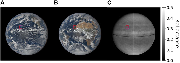
Figure 1. Construction of time-averaged global reflectance maps over an L1B image grid. The DSCOVR spacecraft drifts near the first Lagrangian point (L1), where the EPIC observes the entire day-lit Earth every 1–2 h (13–22 images per day). (A–B) Conventional composite EPIC images for 21 September 2022, 21:54 UTC, and 21 September 2022, 12.54 UTC; SEVs: 10.58° and 10.54°; distances to Earth 1,491,464 km and 1,490,357 km, respectively. All images are 2,048 × 2,048 pixels. (C) “Long-exposure” average image at 780 nm, obtained as a sample arithmetic mean of all individual image reflectances that occur at a given pixel, schematically represented by a red box. The red boxes are pinned to the same spot on the image grid throughout the last 2 weeks of observations in September 2017 (EPIC had a data gap during the first half of the month). Black lines in (C) demarcate the astronomical Equator on 1 September (lower line) and 30 September (upper line). The white cross-hairs are exactly in the middle of the image: 1,024 pixels on either side. L1 positioning secures consistent observing conditions and comprehensive space/time coverage for DSCOVR/EPIC averaging. This differs from geostationary and polar orbiting satellite observations: the former monitors the same place at different times, while the latter views different places at the same local time.

Next, we discuss the explicit construction of the proposed averaging and refer the reader to the red square in all three panels of Figure 1. Although the square represents a single pixel, the size is greatly exaggerated for visual clarity. The grid coordinates of the pixel remain fixed with respect to the image frame (grid) as Earth spins underneath, and whatever part of the globe happens to be at the spot at the time of the next image acquisition gets recorded as the reflectivity of that pixel. Thus, the pixel forms an observation “window” (see Figure 1), averaging a time sequence of reflectivities roughly at the same latitude. This is carried out for all 2,048 × 2,048 pixels and hundreds of images, at a fixed wavelength of 780 nm, in Figure 1C, and the background of no data is rendered black. Hence, Figure 1C is a monochrome (such as an X-ray or electron microscope) “long-exposure” image obtained as a sample (arithmetic) mean of all individual image reflectances that occur at a given pixel (red boxes are pinned to the image grid) during September 2017. This average can also be regarded as that over longitude, and the resulting maps convey the latitudinal dependence of reflectivity. To recap, Figure 1C is a result of averaging in time (over an “ensemble” of images), resulting in longitudinally averaged reflectance, as detailed in the Figure 1 legend.

To get a feel for the DSCOVR EPIC observational circumstances and toward interpreting Figure 1C, we consider a hypothetical “minimal planet” model of a single feature, such as a solitary equatorial island surrounded by a free ocean surface elsewhere. What kind of average image would one expect to see from this schematic planet in Figure 1C? The sampling frequency with which the images are acquired enters the picture now. Indeed, suppose that the island is observed at 7 a.m. local time and that the images are acquired instantly, for a given wavelength, and exactly at 2-h intervals. Then, the image of the island reappears at 9 a.m., 11 a.m., 1 p.m., 3 p.m., and 5 p.m., local time, six in total, throughout the sunlit face of Earth. During the 2 h, Earth rotates approximately 3,000 km, and if our island is that wide, an apparent strip of land around the entire equator is the result. If the island is narrower, the six-pack of islands persists. Over a large number of sampled images, spacecraft hovering about L1 and viewing Earth at different angles, as well as deviations of the sampling frequency from the exact bi-hourly rate, cause blurring of the average images, eventually resulting in a continuous strip of land. Thus, as discussed below, one expects Jupiter-like bands of various features, such as the near-equatorial bright band in Figure 1, caused by the clouds of the inter-tropical convergence zone (ITCZ).

Because Earth contains many types of surfaces, the overall average images are less straightforward to interpret, and this led us to introduce conditioning on surface type so that additional constraints yield greater clarity. Indeed, it turned out that introducing averages conditioned upon cloud presence and/or surface type (e.g., land, ocean, and clouds) at a given pixel yields major improvements in clarity, as shown in Figures 2–4 and discussed in the next section. Such conditioning involves land/ocean and cloud masks. For example, our definition of an ocean surface is the geological one because it is based on a land mask. Thus, an ocean surface pixel mostly but not always implies a water-surface pixel. Thus, in Figure 2, Ross and ice shelves within Antarctica are classified as ocean rather than land pixels, according to the 0.05° latitude–longitude resolution global map of surface cover provided in the MCD12C1 product of the MODIS instrument (DOI: 10.5067/MODIS/MCD12C1.006) (Friedl and Sulla-Menashe, 2015). This is the land mask used in the construction of Figure 2 and subsequent images.

Figure 2

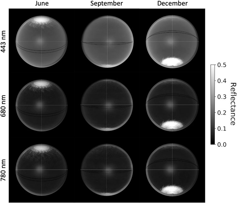
Figure 2. Time-averaged DSCOVR EPIC reflectance images (maps) constructed using cloud-free ocean pixels only. For a given pixel (window of averaging), as Earth spins underneath, reflectance contributes to the aggregate (sample mean) only if the ocean is present and clouds are absent. Thus, the number of contributing images N varies from pixel to pixel. The figure is designed to display climatic and atmospheric effects, and viewing is approximately from the solar vintage point. The columns (months) illustrate seasonal progression due to the tilt of the Earth’s spin axis: different views of polar ice/snow cover are obvious. The rows (wavelengths) display atmospheric (Rayleigh λ⁻⁴) scattering, with the highest reflectances for the blue channel, centered at 443 nm.

Figure 3

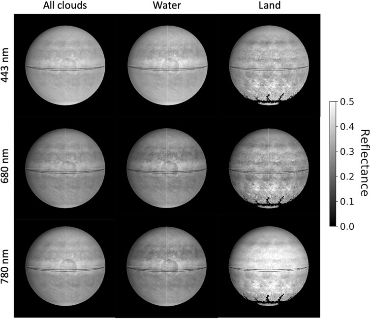
Figure 3. Monthly reflectances in the presence of clouds. At a given image and pixel, reflectance contributes to the sample mean reflectance only if clouds are present at the pixel at that time. The dataset is from all EPIC images collected throughout September 2017. The figure is designed to show an application to cloud detection via effects induced by ocean glitter, as shown by the middle column (oceanic clouds only): the gray circle in the center is most prominent there. This confirms, via a different route, ocean glitter interference with cloud retrievals, in broad agreement with Zhou et al. (2021) and Várnai et al. (2023).

Figure 4

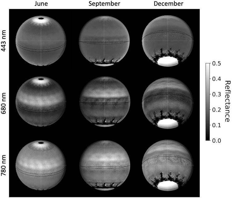
Figure 4. Monthly reflectances for clear land pixels. Earth masquerading as Jupiter; latitudinal bright bands are caused by features such as the Sahara and Antarctica. Black spots are due to the lack or dearth of clear land pixels at that latitude. Repeated spots within latitudinal bands reflect roughly bi-hourly image sampling.

Time-averaged global reflectance maps, conditioned on cloudiness or terrain type

We begin with the time-averaged images of the ocean only, that is, for a given pixel grid location, excluding all images containing (geological) land at a given pixel and all cloud-containing images as determined by the EPIC cloud mask (Zhou et al., 2021). Hence, the number of contributing reflectances varies from one pixel to another (see Appendix). The result is shown in Figure 2, where the conditioning is such that reflectance from a given image contributes to the sample mean only if there is a cloud-free ocean surface within a given pixel as the sunlit Earth spins underneath. The three rows in Figure 2 are for the three wavelengths indicated in the legend, and the Rayleigh effect of atmospheric scattering is evident in the overall brightness. In accordance with the “blue-sky” Rayleigh λ⁻⁴ scattering (with λ denoting the wavelength), the atmosphere is brightest at 443 nm. The bright snow-covered regions at the north and south poles are beacons of the seasonal progression due to the tilt of the Earth’s axis, as one compares the three columns of Figure 2. The black lines again demarcate equatorial lines at the beginning and end of the month.

Figure 2 shows three prominent features involving seasons, orbits, and ocean waves. These features are (i) bright polar caps (of which the spatial extent depends on the time of the year); (ii) the presence of bright edges (left in June and right in December); and (iii) the central bright spot. Before interpreting these features, one must be cautioned that these 1-month “exposure” images are “blurred” by the variable distance and angle between spacecraft and Earth because the spacecraft hovering around L1 causes modestly variable viewing geometry (Valero et al., 2021). For example, because of the DSCOVR Lissajous (halo) orbit about L1, the angular size of Earth varies during the 6-month orbital quasi-period from 0.45° to 0.53°. Similarly, the Sun Earth Vehicle (SEV) angle ranged from 6.75° to 10.25° in 2017. Recall that SEV = 180°—scattering angle between the solar and viewing directions. This blurring is examined briefly in the Appendix on the same data as in the bottom left panel of Figure 2 (cloud-free ocean pixels only) and found not to affect the interpretation significantly. Therefore, without image processing beyond the averaging of L1B data, we continue with the interpretation of the features (i)–(iii).

The brightest areas in Figure 2 are the snow-covered polar “ocean” regions, and, to a first approximation, the viewing direction here can be taken as that from the Sun. Then, the progression of the polar area reflectivity illustrates beautifully the physics of seasons based directly on satellite data. Although the theory of seasonal dependence is textbook material, to the best of our knowledge, no single simple display of this based on direct data (here, EPIC level 1B or L1B) exists. This Figure 2 type of display could enter textbooks as direct data-based evidence of seasonal patterns, yet it is possibly simple enough to be comprehensible to a high school student.

For example, let us focus on the middle column of Figure 2, taken during September, near the fall equinox. There is symmetry here between the Northern and Southern Hemisphere averages, and the Earth’s spin axis is perpendicular to the viewing direction. The left–right (dawn–dusk) symmetry also holds at equinoxes, even though the Earth’s obliquity (axial tilt) is $\approx 23.5°$. The effect of the obliquity, however, is made obvious by Figure 2 construction in June and December, during the summer and winter solstices, respectively. For instance, the Earth’s axial tilt brings, say, the North Pole toward the viewer in June and away in December. Such images may become a valuable tool for data-driven educational outreach.

Turning to item (ii) now, initially, we thought that the appearance of the moving bright edges in Figure 2 was entirely due to the effects of the viewing geometry (Su et al., 2018). Indeed, on closer inspection of individual EPIC images, one can discern partial occlusion via the darkened limb on, say, the eastern side of the globe and a brighter Western rim on the opposite side. However, time averaging brings out the edge effects more prominently. Let us again focus on the middle column of Figure 2, taken during September (near the fall equinox). As mentioned above, when the viewing direction is from the Sun, there is symmetry between the North and South Hemispheres during the equinox (the Earth spin axis is perpendicular to the viewing direction from the Sun), and there is also East–West (dawn–dusk) symmetry, but only to a first approximation, when the viewing direction is from the Sun. However, the spacecraft is always a few degrees off that direction, and therefore, more of the atmosphere is traversed during September at the Western edge than in the Eastern one, thus brightening the right edge in the central panel of Figure 2 and darkening the left limb (see also Figure 3 in the study by Valero et al. (2021). Dawn and dusk no longer correspond to the exact left and right edges of the Earth disk image when the spacecraft camera is not positioned exactly on the Sun–Earth straight line.

As the satellite hovered about the L1 point along its halo orbit in 2017 (approximately a Lissajous figure), it crossed the Sun–Earth axis, which is why the bright edge flipped to the east in June and December of 2017, as shown in the left and right columns of Figure 2. This interpretation is also in agreement with the simulations in Figure 3 from the study by Zhou et al. (2021), which also pertains to September 2017. Although the authors did not comment on it, there is a noticeable asymmetry in the dark blue curve for the cloud-free case.

Upon further examination, we discovered that it is the spacecraft hovering about the L1 point with different views of dawn and dusk, amplified by the cloud mask, that likely contributes to the bright-edge phenomenon. The various contributions to this in detail are addressed in the Appendix, and here, we confine ourselves merely to noting that the bright edges are present only in cloud-free images, as shown in Figures 2, 4, but not in cloudy images, as shown in Figure 3. More generally, the bright edges are prominent in neither the cloudy composite images nor the all-sky composite (combining data with and without clouds) images. All three of the present authors noted the edge effect in regular daily EPIC images only after discovering it in Figure 2. When truly unconditional averaging is performed (as in Figure 1C), clouds tend to dominate scattering by being the most reflective objects. No cloud detection algorithm is invoked in processing these unconditional images. Clouds then restore East–West symmetry, and the bright slivers around the rim are no longer discernible. We remark, in passing, that the notions of sunrise and sunset are associated with the temporal uncertainty of approximately 2 min required to traverse the 0.5° angular size of the Sun (at the hourly angular speed of 360°/24). During this time, the Earth’s surface moves approximately 50 km or 4–5 pixels. This is much less than the width of the bright edges.

Next, we discuss the conspicuous, bright central spot shown in the center of Figure 2. Without clouds, this must be due to ocean glitter. Although not always notable in the individual EPIC images, it was previously detected by Zhou et al. (2021) and thoroughly investigated by them. Originally, we were led to the concept of EPIC image averaging by wanting to extract the ocean glitter feature, as well as glitter elsewhere, by Kostinski et al. (2021). Indeed, the region becomes much more pronounced when conditionally averaged, as shown in Figure 2.

The physics of this specular reflection by suitably sloped ocean waves (tilted wave facets from the geometrical optics perspective) is well understood (Kidder and Haar, 1995; Rees, 2013). The surface is rough insofar as the Rayleigh criterion h_rms ≫ λ, with h_rms being the root mean squared height deviation of the surface and λ the wavelength. As winds ruffle the ocean surface, the bright spot broadens, which permits the extraction of useful information about winds (Cox and Munk, 1954a; Cox and Munk, 1954b). The often-observed glitter reduction by oil and soap suggests that short gravity and capillary waves with wavelengths under 10 cm contribute the most to glitter.

The Cox–Monk expansion around the Gaussian distribution of slopes (Cox and Munk, 1954a) is perhaps the most widespread and currently used roughness characterization (e.g., see the recent results obtained by Guérin et al. (2023)). Open questions remain, however, and difficulties with unrealistic variance were pointed out by Wentz (1976), and mathematical inconsistencies were identified by Tatarskii (2003), who showed that the analytical representation of the Cox–Monk probability density function leads to negative probabilities in certain regions of the slopes. In this regard, merely observing the width of the ocean glitter spot by EPIC may help estimate slope variances directly. In a marvelous effort, Bréon and Henriot (2006) took about nine million measurements, but perhaps EPIC can monitor ocean glitter with much less effort (relatively few images).

To that end, recall that the pixel size near the image center in Figure 2 is ≈ 10 km × 10 km, and the angular width of a pixel is ≈ (3 × 10⁻⁴)°. The conspicuous bright spot is centered on the specular (glint) point, slightly off the middle of the image (Marshak et al., 2017; Várnai et al., 2019; 2023; 2020; Kostinski et al., 2021). The spot is approximately 300 pixels wide. Spacecraft hovering and variable spacecraft-to-Earth distance account for about 15% of the estimated broadening (not shown).

The angular variation in the local surface normal is 0.1° across a pixel or ≈ 15° over the entire bright spot. This translates to ocean surface rms roughness of approximately ± 15° and, therefore, via roughness–wind speed scaling U ≈ (10³σ² − 1)/3 (Bréon and Henriot, 2006; Munk, 2009) (σ denotes the standard deviation of the wave slope distribution) to a ballpark estimate for the wind speed U of approximately 8 m/sec. This is only a rough estimate at the proof-of-concept level, but it does open up the possibility of monitoring secular trends in ocean winds and even testing the windier Earth hypothesis (Zeng et al., 2019). It is also interesting to ask whether the ocean glitter region is circular or somewhat elliptical, as the shape relates to the relative magnitude along cross-wind components and prevailing winds within the ITCZ (Munk, 2009).

Figure 3 is the exact opposite of Figure 2 in that only cloud-containing pixels contribute to the average and also because the central circular spot now turns dark. All clear-sky pixels, regardless of the surface type, are excluded. As expected from an earlier discussion of satellite hovering, clouds in Figure 3 restore symmetry, and bright edges disappear, but at the center, ocean glitter interferes with cloud detection.

The spatial continuity of reflectance is essential here, and, therefore, so is the maintenance of approximately steady illumination and viewing geometry by EPIC. The central spot in the left and center columns is darker, implying a relatively high contribution of darker pixels (scenes). This is likely the result of detecting clouds using a criterion independent of their brightness (oxygen A-band ratios) and thus declaring even relatively dark pixels cloudy in the glint region by the special (designed to overcome glitter interference) cloud mask (Zhou et al., 2021), whereas outside the glint region, cloud detection relies on scene brightness and always places bright pixels in the cloudy category (Yang et al., 2019). As with any perfection, perfect compensation for the presence of interfering ocean glitter when detecting clouds is impossible to attain, but the maps, such as those in Figure 3, may guide monitoring of cloud mask performance. The argument can be inverted to use the spatial cloud mask in order to delineate the region of significant ocean glitter. The land column has no such dark spot because the same cloud mask is uniformly applied there.

Another notable feature of Figure 3 is the presence of bright bands in the land (right) column, somewhat below the 30° latitude. This reflects the high reflectivity of deserts, e.g., the Sahara. For example, the northern region of the middle right panel (680 nm) is brighter than that of water in the middle panel of the image.

The black “spiders” are artifacts caused by the lack or dearth of land-containing pixels near the South Pole. Because of the approximately 2-h image sampling frequency, four or five alternating dark and bright spots are observed on the average image. This apparent periodicity (the “fingerprint” pattern) in the middle panel of the right column is again linked to the approximately 2-h sampling rate of image collection by the EPIC. This leads us to average reflectivity maps exclusively for clear land, as shown in Figure 4, where the sampling periodicity is observed most clearly at 780 nm.

Figure 4 exhibits bright bands at 680 and 780, due to the Sahara, with the Amazonian and African vegetation below the Sahara dark at 680 nm but brightening up at 780 nm. It is interesting to see how the bright bands move northward from June to December, especially at 680 nm. The middle (June) column was collected at a sampling rate of nearly hourly images, thereby leading to more but smaller bright spots. There is no land at the North Pole, which leads to a dearth of contributing pixels, causing image artifacts with occasional black spots. Similarly, there is a band north of Antarctica without land, also exhibiting black spider-like artifacts. The periodic “smudges” are once again due to the sampling frequency of capturing images. For example, imaging every 2 h yields approximately six spots per Earth surface, e.g., at 780 nm in September, as shown in Figure 4, but the image-capturing frequency is slightly higher in June, and one can see the spots diminish in size to a certain extent as the spacecraft hovers further away from Earth during that time.

Figure 4 shows that land is more informative in spectral texture than the ocean or clouds. Sunlight absorption of healthy green leaves dominates the reflectance spectrum at 680 nm: chlorophyll pigments absorb red wavelengths for photosynthesis. On the other hand, there is high reflectance of vegetation at 780 nm: about 50% of the NIR light is reflected.

Concluding remarks

This is a proof-of-concept paper insofar as the concept of an average EPIC image is introduced; extracting a signal (e.g., longer-term trend) from noise (geographic details) is shown to yield useful and interesting insights. The new notion employs synthesis and integration and leads to striking maps likely to contribute, among other things, to educational outreach based on real data. The unique observational circumstances of DSCOVR/EPIC, along with the average reflectance maps, can help with the first Lagrangian point-based solar radiation management via geoengineering (Szapudi, 2023). A set of, say, monthly reflectance maps in various surface conditions has the potential to become a visual manifestation of an atlas or almanac.

Although the pixel size and the lighting conditions of a given grid pixel change from sample to sample, other pixels also experience this, and it is the relative reflectance pattern and spatial continuity of the averages that contain most of the information. Because the same gray-scale assignment is maintained throughout the work, continuity of the resulting time-average reflectivity lends itself to monitoring cloud mask performance and provides guidance on whether and where improvement is needed, e.g., detection of clouds over the ocean glitter region. Indeed, the continuity of the averaged reflectance maps is an attribute that makes them a diagnostic tool. One could even invert the argument to delineate the area of ocean glitter and use the result toward monitoring average winds.

Data availability statement

The original contributions presented in the study are included in the article/Supplementary Material further inquiries can be directed to the corresponding author.

Author contributions

AK: conceptualization, formal analysis, funding acquisition, investigation, methodology, writing–original draft, and writing–review and editing. AM: formal analysis, funding acquisition, investigation, methodology, project administration, resources, visualization, and writing–review and editing. TV: conceptualization, data curation, formal analysis, funding acquisition, investigation, methodology, software, validation, visualization, and writing–review and editing.

Funding

The author(s) declare that financial support was received for the research, authorship, and/or publication of this article. This work was supported in part by the NASA DSCOVR project, ACMAP program, and the National Science Foundation AGS-2217182.

Acknowledgments

The authors thank Karin Blank, Yuekui Yang, Yaping Zhou, and Lilly Kostinski for helpful comments.

Conflict of interest

The authors declare that the research was conducted in the absence of any commercial or financial relationships that could be construed as a potential conflict of interest.

Publisher’s note

All claims expressed in this article are solely those of the authors and do not necessarily represent those of their affiliated organizations, or those of the publisher, the editors, and the reviewers. Any product that may be evaluated in this article, or claim that may be made by its manufacturer, is not guaranteed or endorsed by the publisher.

References

Argenti, F., Lapini, A., Bianchi, T., and Alparone, L. (2013). A tutorial on speckle reduction in synthetic aperture radar images. IEEE Geoscience remote Sens. Mag. 1 (3), 6–35. doi:10.1109/mgrs.2013.2277512

CrossRef Full Text | Google Scholar

Bréon, F., and Henriot, N. (2006). Spaceborne observations of ocean glint reflectance and modeling of wave slope distributions. J. Geophys. Res. Oceans 111 (C6). doi:10.1029/2005jc003343

CrossRef Full Text | Google Scholar

Cox, C., and Munk, W. (1954a). Measurement of the roughness of the sea surface from photographs of the sun’s glitter. J. Opt. Soc. Am. 44 (11), 838–850. doi:10.1364/josa.44.000838

CrossRef Full Text | Google Scholar

Cox, C., and Munk, W. (1954b). Statistics of the sea surface derived from sun glitter. J. Mar. Res.

Google Scholar

Friedl, M., and Sulla-Menashe, D. (2015). Mcd12c1 modis/terra+ aqua land cover type yearly l3 global 0.05 deg cmg v006. nasa eosdis land Process. daac.

Google Scholar

Goodman, J. W. (2007). Speckle phenomena in optics: theory and applications. United States: Roberts and Company Publishers.

Google Scholar

Guérin, C.-A., Capelle, V., and Hartmann, J.-M. (2023). Revisiting the Cox and Munk wave-slope statistics using IASI observations of the sea surface. Remote Sens. Environ. 288, 113508. doi:10.1016/j.rse.2023.113508

CrossRef Full Text | Google Scholar

Kidder, S. Q., and Haar, T. H. V. (1995). Satellite meteorology: an introduction. Houston, Texas: Gulf Professional Publishing.

Google Scholar

Kostinski, A., Marshak, A., and Várnai, T. (2021). Deep space observations of terrestrial glitter. Earth Space Sci. 8 (2). doi:10.1029/2020ea001521

CrossRef Full Text | Google Scholar

Marshak, A., Várnai, T., and Kostinski, A. (2017). Terrestrial glint seen from deep space: oriented ice crystals detected from the Lagrangian point. Geophys. Res. Lett. 44 (10), 5197–5202. doi:10.1002/2017gl073248

CrossRef Full Text | Google Scholar

Munk, W. (2009). An inconvenient sea truth: spread, steepness, and skewness of surface slopes. Annu. Rev. Mar. Sci. 1, 377–415. doi:10.1146/annurev.marine.010908.163940

PubMed Abstract | CrossRef Full Text | Google Scholar

Rees, W. G. (2013). Physical principles of remote sensing. Cambridge: Cambridge University Press.

Google Scholar

Stigler, S. M. (2016). The seven pillars of statistical wisdom. United States: Harvard University Press.

Google Scholar

Su, W., Liang, L., Doelling, D. R., Minnis, P., Duda, D. P., Khlopenkov, K., et al. (2018). Determining the shortwave radiative flux from earth polychromatic imaging camera. J. Geophys. Res. Atmos. 123 (20), 11–479. doi:10.1029/2018jd029390

CrossRef Full Text | Google Scholar

Szapudi, I. (2023). Solar radiation management with a tethered sun shield. Proc. Natl. Acad. Sci. 120 (32), e2307434120. doi:10.1073/pnas.2307434120

PubMed Abstract | CrossRef Full Text | Google Scholar

Tatarskii, V. I. (2003). Multi-Gaussian representation of the Cox–Munk distribution for slopes of wind-driven waves. J. Atmos. Ocean. Technol. 20 (11), 1697–1705. doi:10.1175/1520-0426(2003)020<1697:mrotcd>2.0.co;2

CrossRef Full Text | Google Scholar

Valero, F. P., Marshak, A., and Minnis, P. (2021). Lagrange point missions: the key to next generation integrated earth observations. dscovr innovation. Front. Remote Sens. 2, 745938. doi:10.3389/frsen.2021.745938

CrossRef Full Text | Google Scholar

Várnai, T., Kostinski, A. B., and Marshak, A. (2019). Deep space observations of sun glints from marine ice clouds. IEEE Geoscience Remote Sens. Lett. 17, 735–739. doi:10.1109/lgrs.2019.2930866

CrossRef Full Text | Google Scholar

Várnai, T., Marshak, A., Kostinski, A., Yang, Y., and Zhou, Y. (2023). Impacts of sun glint off ice clouds on DSCOVR EPIC cloud products. IEEE Trans. Geoscience Remote Sens. 62, 1–11. in review. doi:10.1109/tgrs.2024.3400253

CrossRef Full Text | Google Scholar

Várnai, T., Marshak, A., and Kostinski, A. B. (2020). Deep space observations of cloud glints: spectral and seasonal dependence. IEEE Geoscience Remote Sens. Lett. 19, 1–5. doi:10.1109/lgrs.2020.3040144

CrossRef Full Text | Google Scholar

Wentz, F. J. (1976). Cox and Munk’s sea surface slope variance. J. Geophys. Res. 81, 1607–1608. doi:10.1029/jc081i009p01607

CrossRef Full Text | Google Scholar

Yang, Y., Meyer, K., Wind, G., Zhou, Y., Marshak, A., Platnick, S., et al. (2019). Cloud products from the earth polychromatic imaging camera (epic): algorithms and initial evaluation. Atmos. Meas. Tech. 12 (3), 2019–2031. doi:10.5194/amt-12-2019-2019

PubMed Abstract | CrossRef Full Text | Google Scholar

Zeng, Z., Ziegler, A. D., Searchinger, T., Yang, L., Chen, A., Ju, K., et al. (2019). A reversal in global terrestrial stilling and its implications for wind energy production. Nat. Clim. Change 9 (12), 979–985. doi:10.1038/s41558-019-0622-6

CrossRef Full Text | Google Scholar

Zhou, Y., Yang, Y., Zhai, P.-W., and Gao, M. (2021). Cloud detection over sunglint regions with observations from the earth polychromatic imaging camera. Front. Remote Sens. 2, 690010. doi:10.3389/frsen.2021.690010

CrossRef Full Text | Google Scholar

Appendix:Some implications of spacecraft hovering about L-1

As DSCOVR orbits around the L1 point with a roughly 6-month pseudo-cycle, it views the Earth from a slightly changing vantage point. As DSCOVR gets closer, the size of the Earth disc increases in EPIC images. To explore this roughly 10% effect, we developed a simple adjustment to keep the apparent image size of Earth the same in all EPIC data and the visual inspection of monthly composites discussed in this paper was hardly affected. Therefore, for this proof-of-concept presentation, we chose to present image composites based on raw (not size-adjusted) EPIC data as it can be more readily reproduced by others.

Although initially suspecting otherwise, we learned that the size changes do not cause the high reflectances observed near the edges of the Earth disk in Figures 2, 4. Rather, it is the interplay of the viewing geometry and the cloud mask. Several arguments support this conclusion. First, the bright edges occur only in clear-sky composites (Figures 2, 4) but not in all-sky or cloudy-sky composites (Figures 1C, 3), even though the size of the Earth disk changes in the latter composites as well. Second, the high reflectances occupy a much wider region than the range of Earth disk size variability. (In Figures 2, A1, the bright edges are much wider than the range of equator line ends, indicating the size of the Earth disk at the beginning and end of each month). Third, we found that many more EPIC images contribute to each pixel of the clear-sky composites at the bright edges than elsewhere in the Earth disk (Figure A2). This occurs because, due to the grazing solar and viewing angles, clear skies are expected to be much brighter near the edges than well inside the Earth disc [see the blue line in Figure 3 of (Zhou et al., 2021)]. As a result of this expectation, near the edges the EPIC cloud masking algorithm will deem pixels clear even if they have a fairly high reflectivity. Adding these bright pixels into the clear sky composites brightens the edge regions in Figures 2, 4. Closer inspection reveals that the bright edges are somewhat asymmetric: They are brighter on the right side in September and on the left side in June and December (Figure 2). The varying asymmetry occurs because EPIC views the Earth off to one side or the other as it drifts around the L1 point. This causes the opposite edges of Earth to have slightly different ranges of zenith angles and thus slightly different expected clear-sky reflectances [this asymmetry is clearly visible for the blue line in Figure 3 of (Zhou et al., 2021)].

FIGURE A1

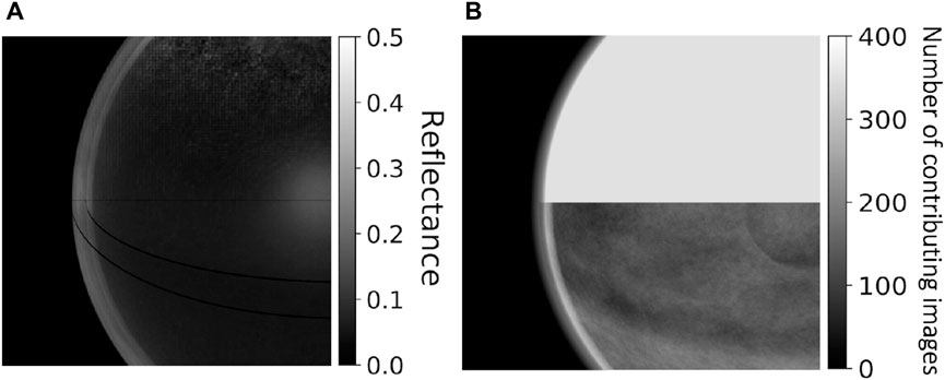
FIGURE A1. Origin of Bright Edges. Similarly to the bottom left panel of Figure 2, (A) shows the 780 nm mean reflectance over clear ocean for June, 2017. Aside from zooming in on the edge, this panel differs from Figure 2 in that the equator lines are not for June 1 and June 21 (northernmost and southernmost equators within the month), but for June 1 and June 30 (when DSCOVR is closest and farthest to Earth, respectively.) The figure shows that the bright edge extends well inside the range of Earth disk size variations indicated by the end points of the equator lines. (B) zooms in the same region but shows the number of images used by cloud mask towards monthly mean reflectance. The top half shows the number of reflectances contributing to all-sky composites (land and ocean, clear and cloudy) while the bottom half shows the number contributing to clear-sky only composites. The number of contributing clear-sky reflectance values is seen to increase sharply well inward from the range of the Earth disk variation (that is, inward from the transition zone seen in the top half of the image). Since the number of clear images increases at locations where the overall image number is still constant, this implies that the cloud masking algorithm classifies a higher fraction of cases as “clear sky” at these locations. The explanation is given in the main text of the Appendix.