Co-located OLCI optical imagery and SAR altimetry from Sentinel-3 for enhanced Arctic spring sea ice surface classification

The Sentinel-3A and Sentinel-3B satellites, launched in February 2016 and April 2018 respectively, build on the legacy of CryoSat-2 by providing high-resolution Ku-band radar altimetry data over the polar regions up to 81° North. The combination of synthetic aperture radar (SAR) mode altimetry (SRAL instrument) from Sentinel-3A and Sentinel-3B, and the Ocean and Land Colour Instrument (OLCI) imaging spectrometer, results in the creation of the first satellite platform that offers coincident optical imagery and SAR radar altimetry. We utilise this synergy between altimetry and imagery to demonstrate a novel application of deep learning to distinguish sea ice from leads in spring. We use SRAL classified leads as training input for pan-Arctic lead detection from OLCI imagery. This surface classification is an important step for estimating sea ice thickness and to predict future sea ice changes in the Arctic and Antarctic regions. We propose the use of Vision Transformers (ViT), an approach adapting the popular deep learning algorithm Transformer, for this task. Their effectiveness, in terms of both quantitative metric including accuracy and qualitative metric including model roll-out, on several entire OLCI images is demonstrated and we show improved skill compared to previous machine learning and empirical approaches. We show the potential for this method to provide lead fraction retrievals at improved accuracy and spatial resolution for sunlit periods before melt onset.

1 Introduction

1.1 Sea ice and leads

Sea ice is constantly in motion as it is subjected to the forces resulting from the surface wind, ocean and internal mechanical stresses (e.g., Heorton et al., 2019). This mobility can result in ice deformation and divergent fracturing forming open water between the ice floes known as ‘leads’. Leads are transient features and can rapidly disappear due to refreezing in winter or due to the sea ice rearranging around them. Hence they encompass the complex thermodynamical and dynamical effects inherent to the very nature of sea ice. Leads are the windows to the ocean in ice-covered regions and in polar altimetry are essential for sea surface height and sea ice thickness retrievals.

Understanding and monitoring the formation and evolution of leads provides valuable insights into the broader sea ice processes and their interactions with both atmospheric and marine systems. Leads in winter influence the local and global climate by altering the exchange of heat and moisture fluxes between the ocean and the relatively colder winter air temperatures (Marcq and Weiss, 2012). In the pack ice, leads only cover 1%–2% of the ocean during winter, but can explain more than 70% of the upward heat fluxes, as confirmed by satellite observations and lead permitting high resolution models (Hutter and Losch, 2020; Ólason et al., 2021).

In summer, leads allow for increased absorption of solar radiation, resulting in enhanced basal and melting of sea ice. The relatively low albedo of open water in leads (≃ 0.1) relative to snow-covered sea ice (≤0.8) (Perovich et al., 2002), allows for greater absorption of solar radiation in leads vs. the surrounding ice. This difference affects the Arctic’s heat budget and can influence weather patterns and ocean currents; just a 1% decrease in sea ice concentration due to a greater fraction of leads has the potential to escalate near-surface temperatures in the Arctic by 3.5 K (Lüpkes et al., 2008).

Leads make other important contributions. They are the place where frazil ice accumulates (Wilchinsky et al., 2015); they are the main source to atmospheric sea salt, originating from frost flowers that grow on ice-covered sections (Kaleschke et al., 2004); they serve as vital hunting areas for marine mammals; and are essential pathways for shipping (Massom, 1988). Accurately detecting leads from satellite observation is therefore crucial for enhancing our understanding of sea ice theromodynamics and dynamics, which in turn is vital for better predicting weather patterns, understanding marine ecosystems, and planning maritime operations in polar regions.

1.2 Leads from space

Identifying leads is a critical step in satellite altimetry for retrieving sea level and freeboard (Quartly et al., 2019). In the winter this classification is based on the radar echo shape via empirical methods using a fixed threshold of key features, such as the leading edge width, pulse peakiness, and stack standard deviation or more recently on machine learning approaches utilising the full echo shape in supervised or unsupervised classification techniques [(Lee et al., 2018) and references therein]. Detecting leads in summer using CryoSat-2 was made first possible using a 1D convolutional neural network (Dawson et al., 2022), which led to the first full year sea ice thickness product from radar altimetry (Landy et al., 2022). Similar work with ICESat-2 has shown that it is possible to detect leads using the full photon cloud properties as part of the official ATL07 product based on a decision tree algorithm (Petty et al., 2021) or with more advanced data-driven ML approaches (Koo et al., 2023). Lead and ice retrievals were then used to characterise lead (frequency, size) (Wernecke and Kaleschke, 2015) and sea ice (floe size, concentration) characteristics (Horvat et al., 2019; Horvat et al., 2023). Here, our lead definition follows winter/spring lead classification of Lee et al. (2018) which is based on a waveform mixture algorithm trained with selected echo characteristics and visually validated with SAR collocated imagery.

Since the 1990s, satellite sensors have become the primary tool for monitoring leads across the Arctic region, with early efforts utilizing the Advanced Very High Resolution Radiometer (AVHRR) and Defense Meteorological Satellite Program (DMSP) to capture visible and thermal imagery of leads (Lindsay and Schweiger, 2015). More recently, the Moderate Resolution Imaging Spectroradiometer (MODIS) has been employed to detect leads using its ice surface temperature (IST) product, which boasts a 1 km spatial resolution, enabling the mapping of pan-Arctic lead presence (Willmes and Heinemann, 2015a). This advancement was further enhanced by the implementation of a fuzzy cloud artifact filter to reduce cloud interference and the analysis of lead dynamics through comparisons with various Arctic Ocean characteristics, including shear zones, bathymetry, and currents.

Despite the high spatial resolution offered by optical sensors, their effectiveness is limited during the polar nights of December to February due to darkness and is further compromised by cloud contamination. To overcome these limitations, microwave instruments such as passive microwave sensors and altimeters have been adopted for lead detection, offering the ability to generate lead fractions even in challenging conditions (Kaleschke et al., 2004).

In recent years, the integration of machine learning (ML) and other forms of artificial intelligence (AI) into the field of remote sensing has significantly enhanced the detection and analysis of sea ice and leads. The recent adoption of ML methodologies in detection of sea ice characteristics reflects the rapid development of deep learning models that can interpret multifaceted satellite imagery/altimetry data. Many studies (Asadi et al., 2020; Han et al., 2021; Khaleghian et al., 2021; Ren et al., 2021; Liang et al., 2022; Huang et al., 2024) exemplify the forefront of this research, demonstrating the application of entropy-based models and deep neural networks in enhancing the detection capabilities for sea ice and leads.

We note also studies that focus on lead detection from moderate resolution thermal infrared (IR) satellite imagery (Willmes and Heinemann, 2015b; Hoffman et al., 2021; 2019; Reiser et al., 2020; Qu et al., 2021). Others investigate the use of satellite imagery from Landsat (30 m) resolution to assess the accuracy of sea ice concentration products (Kern et al., 2019). Generally, high resolution optical (Muchow et al., 2021; Denton and Timmermans, 2022), microwave (von Albedyll et al., 2023; Guo et al., 2022) or even thermal (Qiu et al., 2023) imagery is limited to validation and regional studies due to its smaller coverage and light and cloud limitations. In comparison, OLCI offers a good compromise between resolution (300 m) and coverage (3 days pan-Arctic coverage), with the additional advantage of being colocated with the altimeter Synthetic Aperture Radar Altimeter (SRAL).

1.3 AI methods

In this paper, we propose an innovative approach to sea ice classification from satellite optical imagery that focuses on the utilisation of Vision Transformers (ViT) (Dosovitskiy et al., 2020). Unlike convolutional neural networks, ViTs leverage self-attention mechanisms to capture dependencies between image patches, providing a more nuanced understanding of the complex structures within sea ice and leads. Our method applies the transformative power of deep learning to classify sea ice and leads, a task that has been challenging for algorithms including K-Means Clustering, Random Forests, CNNs, etc. In the growing field of remote sensing for polar studies, several works have leveraged machine learning techniques to address challenges posed by the Earth’s ice-covered regions. For instance (Bij de Vaate et al., 2022), employed an array of supervised and unsupervised machine learning algorithms to detect fractures, or ‘leads’ in sea ice in the Arctic Ocean using Sentinel-3 Synthetic Aperture Radar Altimeter data. They reported high accuracy of up to 92.74%, especially when altimetry observations included measurements from the open ocean. Their study highlights the limitations of current classifiers during the summer months. Similarly (Mugunthan, 2023), underscored the importance of satellite radar altimetry and the use of machine learning algorithms for monitoring lake ice conditions, emphasising its impact on weather, climate, and northern communities. While their focus was not on sea ice, their work elucidates the broader applications and utility of remote sensing technology in Earth Science. This growing number of studies indicates the burgeoning potential and existing limitations of machine learning and remote sensing technologies for ice monitoring, thereby setting the stage for our current investigation.

In this study, our overarching aim is to evaluate the effectiveness of ViTs in classifying different surface types within winter sea ice conditions. Specifically we intend to use the SRAL classification of leads and sea ice as input feature for a ViT model using the 21 OLCI optical bands. This approach paves the way for a Spring pan-Arctic lead product using the wide swath of Sentinel-3 OLCI imagery under sunlit conditions. To achieve this, we outline two main objectives: 1) to introduce the methodology of applying ViT models to satellite imagery of winter sea ice; 2) to validate the ViT model’s performance through comparison with traditional machine learning algorithms, incorporating quantitative metrics like accuracy as well as qualitative metrics such as full image roll-out. The latter involves a visual roll-out and expert assessment of classified images to assess how well each model captures spatial structures in sea ice and lead categories, complementing quantitative accuracy metrics for a holistic model evaluation. The paper is structured as follows: first, we introduce the methods used for data collection and model training; then, we present our findings, emphasising both quantitative and qualitative evaluation metrics; finally, we discuss the broader implications of using ViT models in geospatial analysis, particularly in the monitoring of polar regions.

2 Datasets

2.1 Radar altimetry

This research utilises Level 1B data from the Synthetic Aperture Radar Altimeter (SRAL) aboard the Sentinel-3A and Sentinel-3B satellites (Donlon et al., 2012). For over three decades, satellite radar altimetry data have provided information on the state of sea ice in the polar regions [e.g., (Laxon et al., 2003; Lindsay and Schweiger, 2015; Kwok, 2018; Stroeve and Notz, 2018; Kacimi and Kwok, 2021; Landy et al., 2022)]. Satellite instruments provide year-round coverage of these inhospitable regions, and radars operating at microwave frequencies can penetrate cloud cover, unlike laser instruments.

Ku-band satellite radar altimeters currently in operation include: CryoSat-2 (2010 -), HY-2A (2011 -), Sentinel-3A (2016 -), Sentinel-3B (2018 -), HY-2B (2018 -) and Sentinel-6 (2020 -). Data from the Sentinel-3 satellite are used in this study, taking advantage of its payload which includes the Ku-band SAR Radar Altimeter instrument (SRAL) and Ocean Land and Colour Instrument (OLCI). The combination of these two instruments on a single platform provided the opportunity to develop machine learning techniques for the identification of features within OLCI imagery, and to make comparisons with the radar altimeter data Bij de Vaate et al. (2022). The methodology employed in our study mirrors that of this research, albeit with a pivotal inversion in the utilisation of data sources for ground truth labels and input features. Specifically, while prior studies have leveraged Ocean and Land Colour Instrument (OLCI) imagery data to generate ground truth labels and utilised altimetry data to inform input features Bij de Vaate et al. (2022), our approach adopts a converse strategy where we use instead SRAL echoes to generate ground truth labels following the method outlined in Lee et al. (2018). In our research, we harness altimetry data for the generation of ground truth labels, employing OLCI imagery as the primary source for input features.

Synthetic Aperture Radar (SAR) altimetry represents a significant advancement in radar technology, offering innovative means to measure surface topography, especially over oceanic and icy terrains. SAR altimetry enhances along-track resolution through synthetic aperture techniques, allowing for the creation of narrow radar beams (300 m width) without the need for a physically large antenna. This leads to more accurate and detailed surface elevation measurements, even in complex and rapidly changing environments like polar regions. By synthesizing the return signals from multiple pulses, SAR altimetry can capture fine-scale features, such as leads in sea ice or small oceanic waves. This technology has played a crucial role in various satellite missions, improving our understanding of phenomena like sea level rise, ocean circulation, and ice dynamics. The SRAL thematic product is obtained from the Copernicus Dataspace portal https://dataspace.copernicus.eu/.

2.2 Optical imagery

The Ocean and Land Colour Instrument (OLCI) is installed aboard the Copernicus Sentinel-3 satellites, designed as the advancement of the previous Envisat MERIS instrument, provides observation of the spectral composition of radiance emanating from just above the ocean’s surface (Donlon et al., 2012).

Some key features of OLCI are listed below (Donlon et al., 2012):

• Spectral Range: OLCI operates over 21 distinct bands, ranging from the visible to the near-infrared spectrum. This allows for detailed observations of land, water, and atmospheric features.

• Spatial Resolution: The Ocean and Land Colour Instrument (OLCI) on board the Sentinel-3 satellite has an along-track spatial resolution of about 300 m.

• Integration with Other Instruments: OLCI’s combination with other tools like the Synthetic Aperture Radar Altimeter (SRAL) amplifies its capabilities. This synergy results in enhanced monitoring of sea ice, leads, and other crucial elements in polar regions.

In the context of this research, the use of OLCI’s datasets, along with other instruments like SAR radar altimetry, enables the validation of surface classification algorithms and exploration on classification based on optical imagery. Specifically, our training dataset comprises segments of data from March in 2018 and 2019, corresponding to 80 tracks representative of the pan-Arctic March sunlit conditions. This selection constitutes approximately 10,000 data points for training and testing purposes. We used all the 21 bands from OLCI as the input features. The 21 bands provide rich information about oceanic surfaces, offering a comprehensive spectral range that enhances the accuracy and detail of our classification models. All data used in this analysis are available with this paper on Zenodo. The OLCI satellite product is obtained form the Copernicus Dataspace portal https://dataspace.copernicus.eu/.

3 Methods

In this section, we include details of our methodology for identifying leads in OLCI imagery data. We provide details of the vision transformer model that we use for sea ice vs. lead classification, and other baselines for comparing the vision transformer model against. In addition, we provide details on the data preparation method; this uses datasets in Section 2 to generate a labelled dataset for training and testing our models.

3.1 Vision transformer (ViT)

We propose a sea ice vs. lead classification model based on the Vision Transfomer (ViT) architecture (Dosovitskiy et al., 2020) to detect leads from OLCI imagery. ViTs are driven by the powerful Transformer architecture, first introduced by Vaswani et al. (2017) in the context of natural language processing (NLP), to learn complex, non-local dependencies between input tokens (i.e., text input in NLP tasks). While the original Transformer model was developed to handle sequential data, ViTs extend this by taking image patches as input tokens to learn dependencies between different regions of an image. The model architecture of Transformers/ViTs is designed for parallel computing, which enables efficient training on GPUs and fast predictions on large OLCI images. However, they typically require large, diverse training datasets to reach optimal performance (Dosovitskiy et al., 2020).

We train the ViT model on a labelled dataset comprising local patches of OLCI images and the corresponding 0/1 label, indicating whether the corresponding pixel is a sea ice (0) or lead (1). We explain in Section 3.3 the method that we use to generate these labels from co-located SAR radar altimetry data.

In Table 1, we outline the main components that form a general ViT model. This consists of (1) a patch encoder layer, (2) a positional embedding layer, (3) a Transformer layer, and (4) an output Multilayer Perceptron (MLP) layer. We provide brief explanations of each of these below.

Table 1

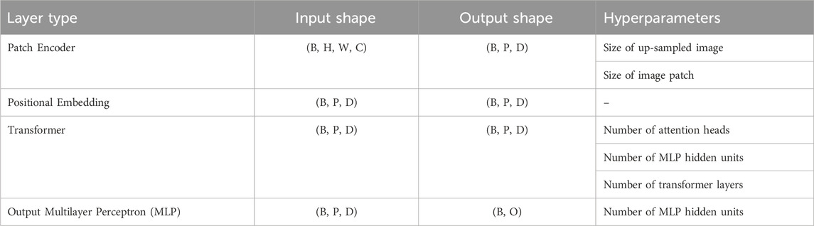
Table 1. General structure of a Vision Transformer (ViT) model. We display the layers comprising a ViT model, the shape of its inputs/outputs, and the layer hyperparameters. For the tensor shapes, we denoted: B - minibatch size, H - image height, W - image width, C - channel size, P - number of patches, D - embedding space dimension, and O - number of output classes.

First, the patch encoder layer takes as inputs images of shape (B, H, W, C), where B is the mini-batch size, H and W are the image’s height and width respectively, and C is the number of channels. The purpose of this layer is to split the input image into a set of P non-overlapping image patches and to encode each of them to a D-dimensional vector via a learnable embedding map. We may choose to up-sample the images first before splitting them up into patches, which may be necessary if the input image is small. The number of patches is then calculated as $P=⌊\frac{\mathtt{i}\mathtt{m}\mathtt{g}\text{\_}\mathtt{x}}{\mathtt{p}\mathtt{a}\mathtt{t}\mathtt{c}\mathtt{h}\text{\_}\mathtt{x}}⌋\times ⌊\frac{\mathtt{i}\mathtt{m}\mathtt{g}\text{\_}\mathtt{y}}{\mathtt{p}\mathtt{a}\mathtt{t}\mathtt{c}\mathtt{h}\text{\_}\mathtt{y}}⌋$ where (img_x, img_y) is the up-sampled image dimensions and (patch_x, patch_y) is the patch dimensions. The channel size C is fixed during the upsampling and splitting steps. Each image patches are flattened before applying the linear embedding map to yield the respective D-dimensional codes, resulting in a tensor of size (B, P, D).

The encoded patches obtained in the first step are then passed through a positional embedding layer, which adds positional information of each of the patches. This is achieved by transforming the indices of the image patches into a D-dimensional vector by a fixed embedding map, and adding it on to the respective D-dimensional encoded patch.

Next, the Transformer layer introduces learnable correlations between the image patches by a so-called multi-head attention mechanism. This processes the encoded patches to generate K new representations of it that take into account its context in relation to the other patches. Here, K is the number of so-called attention heads. The new representations are stacked and passed through a Multilayer Perceptron (MLP) layer with KD-dimensional inputs and D-dimensional outputs. The resulting tensor thus retains the shape (B, P, D). Typically, the patches are processed through several of these transformer layers, to increase the expressivity of the model.

Finally, an output MLP is applied to a flattened output of the Transformer layers to produce the predictions. These consist of probabilities over the target classes, obtained by applying softmax activation in the last layer. Predictions are then made based on which class was assigned the highest probability. For the purpose of regularisation, dropout is applied to the hidden layers of the MLP during training.

For our specific task of classifying sea-ice and leads from OLCI imagery data, since it is a binary classification task, we set the number of output classes to O = 2. Furthermore, we utilise all 21 channels of the OLCI imagery, hence we also fix the channel size to C = 21. For the remaining hyperparameters, we performed a hyperparameter sweep aided by the AI experiment tracking tool Weights and Biases. The resulting configuration that gave the best performance on a held-out validation set is displayed in Table 2. We note that in the “training hyperparameters” row, we display the hyperparameters of the AdamW optimiser used to train the model and the dropout rates used in the hidden layers of the two MLPs – one in the transformer layer and another in the output layer.

Table 2

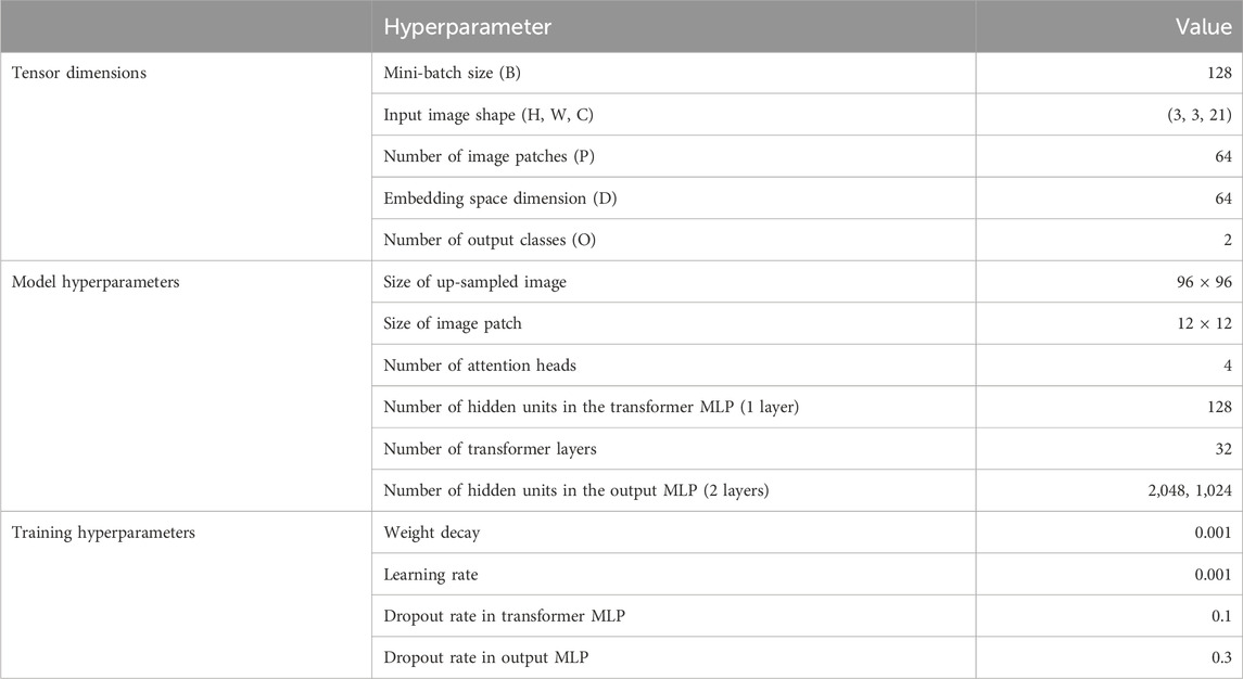
Table 2. The specific ViT configuration that we use in our task of classifying sea-ice and leads in OLCI images. We display (1) the dimensions of the tensors being passed through the layers, (2) the hyperparameters of the ViT model, and (3) the hyperparameters of the training process. See Table 1 for reference. These values are found by performing a hyperparameter sweep aided by Weights & Biases.

3.2 Baseline models

To evaluate the ViT model for sea-ice/lead classification, we compare it against several baselines including standard supervised algorithms (Convolutional Neural Networks, Random forest, MLP), a semi-supervised algorithm (label spreading) and an unsupervised algorithm (K-means clustering). We provide details of each model below. By using a mix of supervised, semi-supervised and unsupervised baselines, we can evaluate the added value of the labelled data generated from SAR altimetry (see the details in Section 3.3). All models were trained on Google Colab, and the CPU/GPU details varied depending on the availability of resources.

3.2.1 Supervised 1: convolutional neural networks (CNNs)

The first baseline model we consider is a CNN model (LeCun and Bengio, 1995) that predicts lead or sea ice from an input image patch. We performed a hyperparameter sweep to find the optimal combination of CNN hyperparameters that generalised best on our validation set. The AI developer platform Weights and Biases was used to facilitate this sweep. The resulting CNN model architecture consists of a single convolutional layer with 64 filters, a kernel size of 3, a stride of size (2,1), and ReLU activation. The output of the convolutional layer is flattened and fed into two dense layers with 64 and 32 units respectively, with ReLU activation in both layers, and a softmax activation applied to the output layer. We use inputs of shape (3,3,21), corresponding to the height, width and channel size respectively of a single input image patch. For training, we used the AdamW optimiser with a learning rate of 0.001 and batch size of 64.

3.2.2 Supervised 2: random forest

The Random Forest (Ho, 1995) model utilises a multitude of decision trees, each voting for a final class label, with the majority vote defining the ultimate prediction. An important attribute of Random Forests is their inherent capability to manage feature interactions and non-linearity. Moreover, they are less prone to overfitting compared to a single decision tree, due to the averaging performed across multiple trees. We used the Random Forest classifier from the scikit-learn library with 21 dimensional input feature vector, corresponding to the 21 channels of a single pixel of an OLCI image. These features are passed through the Random Forest model to determine whether the pixel corresponds to sea-ice or lead.

3.2.3 Supervised 3: multilayer perceptron (MLP)

We also consider a standard MLP model (Murtagh, 1991), tuned using Weights and Biases’s hyperparameter sweep to select the model with optimal performance on our validation set. Our resulting model consists of three dense layers with 300, 100, and 10 units, respectively, with the ReLU activation applied to the first two layers, and a softmax activation in the output layer. As inputs, we used image patches of shape (3,3,21) that is flattened to a 189-dimensional vector. For training, we used a batch size of 32 and the AdamW optimizer with a learning rate of 0.001.

3.2.4 Semi-supervised: label spreading

Label Spreading (Zhu and Ghahramani, 2002) is a semi-supervised algorithm that operates on a given dataset by constructing a fully connected weighted graph, where each data point serves as a node in the graph and the weights on the edges are determined by the affinity of the two data points; the more similar the data, the higher the weight on the edge connecting them. The process then involves propagating labels from nodes that are labelled to those that are not through the edges of the graph. This is done in such a way that a larger edge weight between two nodes indicates a higher likelihood of it getting assigned the same label. We used the implementation for Label Spreading in the scikit-learn Python package.

3.2.5 Unsupervised: K-means clustering

Finally, we consider K-means (MacQueen, 1967) clustering as an unsupervised model to compare our model against. The K-means clustering algorithm forms K distinct clusters by initially selecting K random centroids, then iteratively assigning data points to the nearest centroids and recalculating the centroids as the mean of the points in the clusters. The process continues until convergence, effectively grouping data points with similar attributes by minimising the within-cluster sum of squared distances. In our application, we use K = 2 clusters; one for sea ice and one for leads. We used the Euclidean distance on the 21-dimensional feature space (consisting of the 21 channels of the OLCI image) to define the centroids and assign data points to a cluster. We used scikit-learn’s K-means clustering module for the implementation.

3.3 Generation of labelled dataset

Here, we describe in details how we generate the labels for our dataset, used to train our ViT model and the supervised/semi-supervised baselines described above. We start by collating two sets of data: one containing directories of cloud-free OLCI images with 21 full-resolution top-of-atmosphere (TOA) radiances, and the other containing the SAR data along coincident tracks with the OLCI images. An example of colocation of SAR tracks and OLCI images is illustrated in Figure 1. These are all collected in March in the years 2018 and 2019 over the Arctic Ocean.

Figure 1

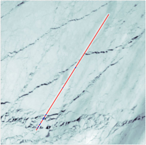
Figure 1. An illustration of a co-located SRAL track and an OLCI image. The colors along the track indicate the predicted labels using the Waveform Mixture Algorithm. Red pixels indicate sea-ice and blue pixels indicate leads.

Before we introduce the procedure of producing labelled dataset, some details of Waveform Mixture Algorithm (Lee et al., 2018) are presented below. The waveform mixture algorithm (WMA) was inspired from the concepts of spectral mixture analysis and it was firstly introduced and employed to lead detection using waveform data from CryoSat-2 for data from Janurary-May and October-December between 2011–2016. Endmember extraction is the process of choosing a set of pure spectral signatures of ground features found in remote sensing data. In this case, endmembers represents the most informative/indicative waveform of a class, such as sea ice and lead. Appropriate selection of endmembers is crucial for spectral mixture analysis (SMA). One of the assumptions of Spectral Mixture Analysis (SMA) is that the spectral data recorded by sensors for a single pixel represents a linear combination of the spectra from all the different components present within that pixel. Spectral mixture analysis identifies the proportions of different components (i.e., classes) in mixed pixels by calculating the abundance of each component based on their endmembers. Since the waveform data inside a footprint can be considered as a mixture of different surface types, for example, sea ice and lead, it is sensible to use SMA/WMA in this context. Calibration and validation were carried out with four visually labeled 250 m resolution MODIS images from March to May and October, ensuring temporal differences with CryoSat-2 data were under 30 min. Reference point data (50% randomly selected from the MODIS data) for leads and sea ice were utilised to set binary abundance thresholds for these two classes through automated calibration. The lead condition thresholds established were a lead abundance greater than 0.84 and a sea ice abundance less than 0.57. The WMA achieves an overall accuracy of 95%. However, this method has a limitation: within a footprint, the waveform may not be a linear mix between sea ice and leads. When both leads and sea ice coexist in a footprint, CryoSat-2 is more responsive to the specular reflection of leads than to the diffuse reflection of sea ice, making the waveform resemble the lead endmember.

According to their documentation, the Sentinel-3 SRAL has specifications very similar to CryoSat-2 SIRAL, including radio frequency and pulse bandwidth, etc (European Space Agency, 2011; European Space Agency, 2022). This suggests that the Waveform Mixture Algorithm (WMA) built for CryoSat-2 can be applied effectively to Sentinel-3 SRAL data, supporting the notion that fine-tuning of the WMA is not necessary.

The lead definition in this study primarily relies on how the Waveform Mixture Algorithm (WMA) classifies the waveform into sea ice and lead. As the WMA is trained and evaluated using 250 m MODIS images, the size of leads in this study can be approximately considered as 250 m. Lee et al., 2018 also states that WMA might have difficulties detecting refrozen leads. Additionally, off-nadir observations can introduce geometric distortions and variations in waveform characteristics. Since the classification algorithm is designed for nadir observations, off-nadir waveform might be interpreted differently, affecting the consistency of our lead labels. These observations exist in our dataset and may complicate the accurate classification of leads. In summary, our definition of lead relies on the Waveform Mixture Algorithm (WMA), which classifies waveform into sea ice and lead based on nadir observations, typically considering lead size as approximately 250 m and primarily focusing on open leads, though off-nadir observations may introduce distortions.

The following procedure is used to produce the labelled dataset to train our models:

1. Using the Waveform Mixture Algorithm (Lee et al., 2018) and the echo measurements from SAR altimetry, produce 0/1 labels along the SAR track, indicating whether a point on the track is a sea-ice (0) or lead (1). An example of such a track is shown in Figure 1.

2. The closest OLCI pixel to each point on the SAR track is identified. For each point along the SAR track, a square patch from the OLCI image with shape (n, n, 21) (height, width, channel) is extracted, centered around the closest OLCI pixel.

3. The TOA radiance values of the OLCI image patch is converted into TOA reflectance using the formula (1) (Sea, 2023; NASA, 2023).

$R_{\text{TOA}}^i=\frac{\pi L_{\text{TOA}}^i}{E_0^i\cos \left(\theta \right)},i=1,\dots ,21,(1)$

where $L_{\text{TOA}}^i$, $R_{\text{TOA}}^i$ denotes the TOA radiance and reflectance respectively on the ith channel, $E_0^i$ denotes the solar flux on the ith channel, and θ denotes the solar zenith angle (SZA).

4. Sub-sample leads and sea-ice in equal proportions to prevent imbalance in data. Note that there will be many more sea ice than leads if we used all of the data generated in steps 1–3, hence making this sub-sampling step necessary.

Once we run steps 1–4 to generate a labelled dataset from our repository of collocated OLCI and SAR data, we split it into a training and test set. We considered a 7 : 3 split, resulting in a total of 9,909 training instances and 4,463 testing instances. Here, each n × n × 21 image patch of TOA reflectance (obtained in Step 3) will be used as input features to the model and the binary labels generated from SAR altimetry (obtained in Step 1) will be the corresponding labels.

4 Results

In this section, we evaluate the performances of the machine learning models considered in Section 3 from both quantitative and qualitative perspectives. First, we assess their accuracy on the labelled test data, providing a quantitative measure of the models’ performances. Second, we roll-out the models on full OLCI images to qualitatively assess the sea-ice/lead segmentation maps that they produce. We will see that performance on one is not necessarily reflected on the other, highlighting the need for both assessment methods. In particular, assessing solely on the test data may produce misleading results as our labelled dataset may contain some bias resulting from how the data was collected.

4.1 Quantitative assessment on the test set

In Table 3, we display the test accuracy of the ViT model and various supervised, semi-supervised and unsupervised baselines on the sea-ice/lead classification task to make a quantitative assessment of the different methods. For the unsupervised and semi-supervied baselines, in addition to the data in the training set, we also utilised 20,000 extra data points collected from the unlabelled areas of the OLCI images. We see that all of the methods have an accuracy of well-above 50%, indicating that the predictions made by them are all significantly better than chance. Therefore the dataset indeed contains signals to distinguish leads from sea-ice. This is also true for the unsupervised model (K-means clustering), which does not use the labels produced in Section 3.3, suggesting that the 21 bands of TOA reflectance values used as model inputs also contain sufficient information to approximately distinguish leads from sea-ice. This agrees with our intuition, since we can visually inspect from the shading of a channel of the OLCI images whether a pixel is sea-ice or lead (see Figure 2 for an example OLCI image). We note that using the original TOA radiance values, the model under-performed significantly. Thus, the post-processing step in Section 3.3 of converting these to TOA reflectances is critical for achieving good performance.

Table 3

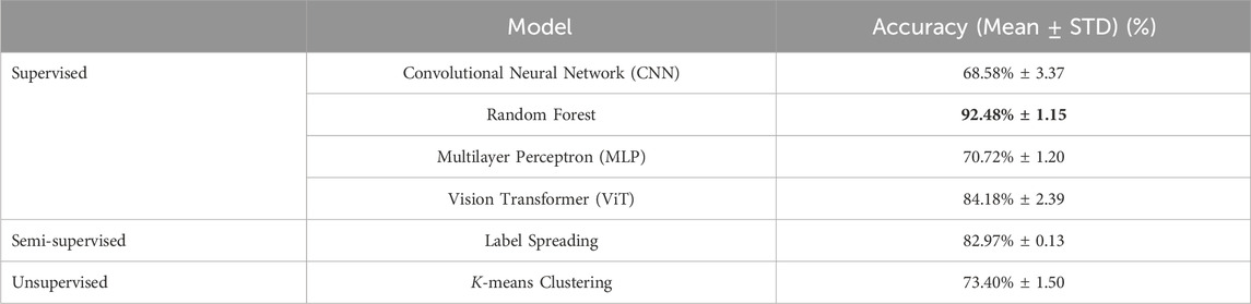
Table 3. Comparison of model accuracies on the labelled test set. We display the mean and standard deviation of the accuracies obtained by training the models from five different random seeds.

Figure 2

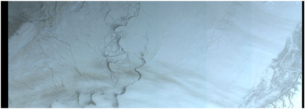
Figure 2. Selected OLCI image that we use to perform our qualitative assessment of the various machine learning models. The selected image has a good mix of sea-ice and leads as well as some areas that are covered by clouds and areas where patches of land are visible.

We also note that the Label Spreading, Random Forest and ViT models all outperform K-means clustering, suggesting that the labels obtained from the SAR altimetry tracks can substantially improve the classification results, justifying our use of it. In particular, we see that the Random Forest model has a performance exceeding 90%, indicating that it has learned a strong relationship between the input TOA reflectance values and the corresponding output classes. However, we see that the other supervised baselines (CNN and MLP) perform worse than the K-means baseline, hence the addition of the labels does not automatically produce better performance and indeed the model choice also plays a crucial role. We see that the ViT model has the second best performance after Random Forest, with a slightly higher accuracy than the Label Spreading baseline, the latter which utilises both supervised and unsupervised techniques to generate predictions. The fact that the ViT and Random Forest model performs better than K-means and Label Spreading indicates that in order to classify a pixel, the information from neighbouring pixels or the corresponding information contained (the labels) in the 21 bands of the TOA reflectance at that pixel is necessary and sufficient to produce good results.

It is however crucial to note that we have only evaluated the classification performance on a pixel-by-pixel basis here, and the task of classifying satellite images involves not only correctly identifying individual pixels, but also preserving the spatial structures and patterns in the images. In addition, since the labels in our curated dataset are themselves not accurate (as they are produced by another model), the results in Table 3 provide only an approximate assessment of the model performances. For these reasons, in addition to the quantitative assessment provided here, in the following we also provide a qualitative assessment by rolling-out the model on a full OLCI image to produce segmentation masks for sea-ice and leads. We will see that while the ViT model has not performed the best in terms of quantitative assessment here, it has significantly better behaviour compared to the other baselines in terms of visual expert assessment.

4.2 Qualitative assessment by full image roll-out

In the context of image processing, image roll-out refers to the process of applying trained models on full-sized images to produce certain outputs, such as a segmentation map covering the entire image. Here, we roll-out our trained models on an OLCI image to provide qualitative assessment of the model performances, comparing their abilities to produce sound segmentation maps for sea-ice/leads.

The OLCI image selected for the roll-out assessment represents a specific geographic area with ample mix of sea ice and leads. The selected image, shown in Figure 2, has a size of 1714 pixels in height and 4,863 pixels in width, resulting in a total of approximately 8.3 million pixels. A variety of spatial structures and patterns are noticeable that reflect the distribution and arrangement of sea ice and leads; notably, we see large contiguous areas of sea ice, interspersed with many fine streaks of leads. In addition, we see clouds over some parts of the image, as well as parts of land that are visible, which may cause additional difficulties in the classification.

Each model in Section 3 is rolled-out on the selected image to produce a segmentation map of leads/sea-ice. These maps provide a visual representation of the model’s classifications, with each pixel colour-coded to indicate whether it has been classified as sea ice or lead by the model. In Figure 3, we display the results of each model, where the black pixels indicate those that are classified as sea-ice and white pixels as those classified as leads. The results show that Random Forest, despite achieving the best accuracy on the test data, demonstrate limited ability to capture the finer lead patterns in the image. In addition, areas where clouds and land are visible are frequently misclassified as leads. The results are similar or worse for the remaining baselines (K-means, CNN, MLP and Label Spreading), with none of them being able to capture fine-scale lead patterns that are present in the image.

Figure 3

Figure 3. Comparison of model roll-out on the select OLCI image. We see that while the random forest model (E) achieved the highest test accuracy, the roll-out results are sub-optimal, failing to detect many of the finer leads on the left side of the image. The other baselines (A–D) also perform poorly, in particular, they have a tendency to misclassify clouds as leads. In contrast, the ViT (F) model does not have this problem, being able to capture the finer-scale leads and being robust to corruption due to clouds.

In contrast, the ViT model, despite having lower accuracy on the test data compared to the Random Forest baseline, demonstrate far superior qualitative result on the full image roll-out. We can claim this since firstly, it is able to detect many finer-scale lead patterns that the other models have failed to capture, and secondly, the predictions are robust to pixels covered by clouds, as it has not misclassified them as leads as the other models have. On the other hand, the ViT model does missclassify parts of land as leads (see the lower-right quadrant), this may imply that the optical features of the land is similar to that of lead, however this is also true for all the baselines considered. This issue will not significantly impact the generation of lead maps for the Arctic region, as all land areas will be excluded from the classification process. Similar to other models, there are some misclassifications in the center-right area of the OLCI image, likely caused by the shadow of the ice ridge. In the future, enhancing and verifying the ground truth labels will be essential to minimise the impact of ice ridges and reduce misclassifications.

A likely reason for the performance discrepancies between the quantitative results in Section 4.1 and the results on the full-image roll-out considered here, is that our labelled dataset is inherently biased, resulting from how we curated the data. For example, in our case, we use labels produced by the Waveform Mixture Algorithm (Lee et al., 2018), which itself is imperfect and therefore introduce errors on the labels. Furthermore, we only extracted data where the pixels over the colocated SAR tracks were relatively cloud and land-free, introducing another source of bias to the curated dataset. Therefore, fitting well on the labelled dataset may also imply that the model has inadvertently fit on the bias that are present in the data, which may actually be detrimental when deploying on a full-sized image. Despite this, it still comes as a surprise that the ViT performs as well as it does on the image roll-out, managing to generalise well on out-of-distribution regimes in the OLCI image. While adversarial robustness in ViTs have been observed in the literature (Zhou et al., 2022), further investigation is necessary to understand why the ViT model generalises better than the other models on image roll-out, despite being trained on the same dataset.

Our findings here highlight the importance of considering multiple evaluation methods when assessing the performance of machine learning and deep learning models. While pixel-level accuracy on the test eset provides an approximate measure of a model’s performance, due to the inherent bias present in the dataset and the fact that it ignores any spatial structure produced, the full image roll-out offers a more holistic view of a model’s ability to reproduce the overall lead structures and patterns in the images.

4.3 Comparison with IRIS: intelligently reinforced image segmentation

To provide some more concrete measure on the qualitative results found in the previous section, we also include comparisons of our results with another method combining human manual labelling and machine learning, specifically, using the Flask app IRIS (Intelligently Reinforced Image Segmentation) (ESA-PhiLab, 2024).

Using IRIS, users can explicitly annotate a small subregion of an unlabeled image via a web interface, assigning labels to pixels. This initial classification made by the user is then processed by a backend model based on Gradient Boosted Decision Trees, which classifies the entire image based on these inputs. This process is then iterated: the users can refine the model’s classification by making corrections and with each iteration, the model learns from these adjustments to update its predictions accordingly. After several rounds of the process, the resulting segmentation map becomes highly accurate. However, in practice, using IRIS is limited to selected images, is time consuming and requires significant human labour, making it impractical for rolling-out on full images. This is where automatic segmentation using machine learning methods such as ViTs are useful, which, once trained, can be used to automatically roll-out on images without requiring human labour. Hence, if we can demonstrate that the machine learning models can achieve similar results as IRIS, then we can potentially deploy it as a practical lead detection tool at a much larger scale (see Section 4.4).

Concretely, our objective here is to use the results produced by IRIS on a small subregion of an OLCI image (shown in Figure 8) as a proxy to the ground truth segmentation map, that we can use to compare our models against. We are aware that similar to the quantitative assessment in Section 4.1, this comparison is also inherently biased, as outputs from IRIS depends on the human labellers used to generate the classifications. Hence, to reduce this bias, we used averaged IRIS outputs from 21 different human labellers as the ground truth proxy. Using this, we can provide a quantitative assessment of the models’ roll-outs by comparing with this proxy.

In Figure 4, we display the average IRIS classification map alongside those generated by ViT, Label Spreading and Random Forest. We see that the ViT produces results that are closely aligned with that of IRIS, detecting virtually all of the leads identified by the latter. This is not true in the case of Label Spreading and Random Forest, which fails to capture some of the finer structures, as well as misclassifying some pixels as leads in the case of Random Forest (see the lower part of the image). However, it is also noticeable that ViT adopts a more generous approach in its classifications, leading to wider leads compared to those in IRIS’s classification. Specifically, some edges of leads that IRIS does not classify as such are indeed classified as leads by ViT.

Figure 4

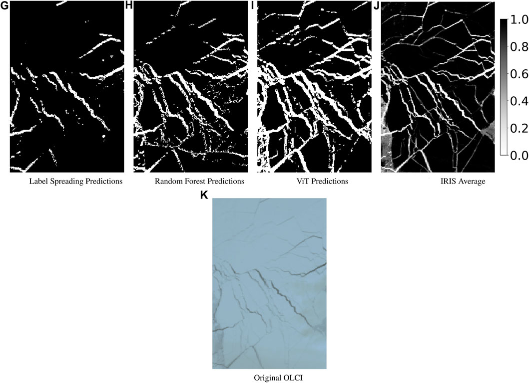
Figure 4. Comparisons of segmentation maps produced by IRIS (J) and other models (G: Label Spreading, H: Random Forest, I: ViT) on a sub-region of an OLCI image (K). For the map produced by IRIS, we display the average across 21 different maps produced by different human labellers for robustness. We see that compared to the other models, ViT can detect virtually all of the leads detected by IRIS, although the labelling is more generous, leading to a bolder segmentation map.

In Figure 5, we also display the confusion matrix with classes 0 and 1 corresponding to sea-ice and leads respectively, detected by IRIS (on the vertical axis) and one of the other models (on the horizontal axis). Here, we see that Label Spreading and Random Forest detects sea-ice more accurately, while ViT detects leads more accurately, with far fewer false negatives for predicting leads. The worse performance of ViT in detecting sea-ice is likely attributed to the generous labelling of leads that we observed earlier. We can furthermore quantify these observations by computing the Precision, Recall and F₁ scores for detecting leads, computed respectively as:

$\text{Precision}=\frac{TP}{TP+FP},\text{Recall}=\frac{TP}{TP+FN},\text{and}{F}_1=\frac{TP}{TP+\frac{1}{2}\left(FP+FN\right)}$

where TP, FP and FN are shorthands for true positives, false positives and false negatives, respectively. This is displayed in Table 4. In short, the Precision quantifies the proportion of detecting leads correctly among all predictions made by the model, the Recall quantifies the proportion of leads being detected correctly among all leads detected by IRIS, and the F₁ is the harmonic mean of the precision and recall. We see that while Random Forest and Label Spreading outperforms ViT in Precision, indicating that ViT misclassifies many sea-ice as leads due to the generous labelling, the Recall score for ViT is near-perfect, indicating that it is able to capture almost all of the leads detected by IRIS. The F₁ scores for all models are similar, with the Random Forest slightly outperforming the other two. Overall, the result suggests that if we place emphasis on labelling leads correctly, then ViT is by far the superior model. However, if we also place emphasis on the precision of the predictions, then ViT still has room for improvement.

Figure 5

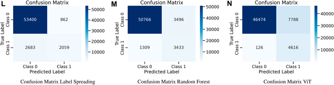
Figure 5. Confusion matrices for comparing the performances of Label Spreading (L), Random Forest (M) and ViT (N) against IRIS. Here, the classes 0 and 1 correspond to detecting sea-ice and lead, respectively.

Table 4

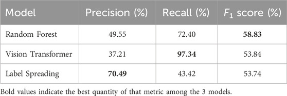
Table 4. Quantitative performance comparisons of Label Spreading, Random Forest and ViT for detecting leads (class 1 in Table 5). We compare the Precision, Recall, and F₁ scores. We see that while Random Forest and Label Spreading has better Precision score than ViT as a result of ViT classifying leads generously, the Recall score for ViT is near-perfect, indicating that it is able to detect almost all of the leads detected by IRIS.

4.4 Mapping of sea ice leads and ice distribution: 2019 march binned map

Finally, we investigate the potential use of the ViT model for generating large scale sea-ice/lead maps by combining the model roll-outs on multiple OLCI images within a given area in the Arctic. This analysis involves dividing the study area into a grid of equal-sized cells or bins, with each cell representing a 1 km² area. For each OLCI image, the geographical coordinates were transformed to a common projection (North Polar Stereographic) to ensure uniformity across the dataset. The transformed coordinates were then used to assign an OLCI pixel and its corresponding prediction (lead or sea-ice) to a grid cell based on its location. Within each bin, we then calculated the following quantities:

1. Lead Count: The number of pixels classified as leads within the bin.

2. Ice Count: The number of pixels classified as sea ice within the bin.

These counts were then used to calculate the fraction of leads in each grid cell, approximately representing the proportion of the cell area covered by open water (leads) as opposed to sea ice. The use of binned statistics allowed us to efficiently process and visualize the large volume of satellite data, providing a clear and quantifiable representation of the lead and ice distribution across the Arctic region. This method also facilitated the handling of overlapping images and the integration of data from multiple satellite passes.

The resulting map in Figure 6 illustrates the fraction of leads in the Arctic sea ice, based on a selection of OLCI images captured during March 2019. We have also performed roll-outs on several images that were not used to generate our labelled dataset. The locations of three examples are marked with coloured rectangles on the binned map in Figure 6 and the corresponding masks for individual OLCI swaths are shown in Figure 7.

Figure 6

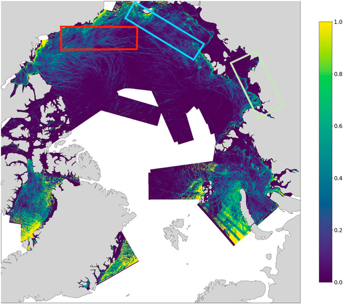
Figure 6. A partial binned map of lead fractions across the Arctic, generated by rolling out the ViT model on multiple OLCI images. The three highlighted rectangles indicate OLCI images that were not used to generate the labelled data. The resulting map demonstrates the ViT’s capability to be used for developing large-scale lead products. Due to hardware constraints, we were not able to use the full OLCI images available to produce a complete map.

Figure 7

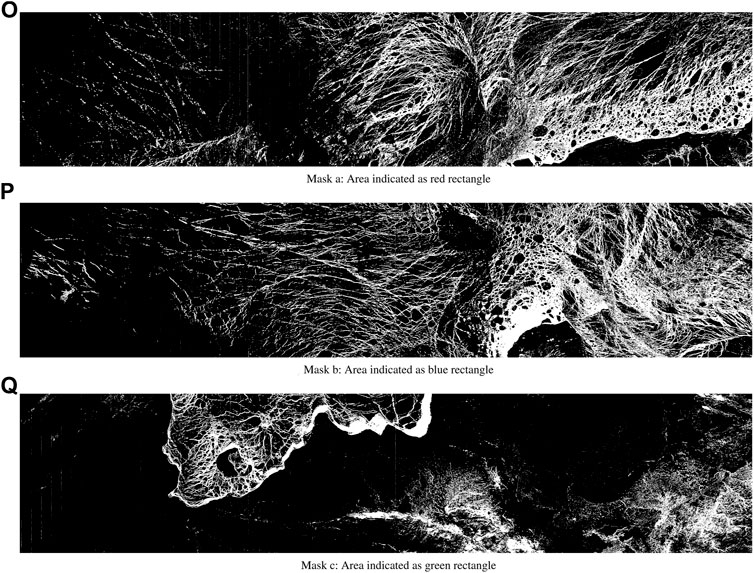
Figure 7. Lead and Ice masks for three selected OLCI swaths indicated by the highlighted rectangles in Figure 6. Namely, regions (O) red rectangle, (P) blue rectangle, and (Q) green rectangle. The ViT produce sound maps for these areas (although they are still influenced by the presence of clouds), despite none of them being used to create the labelled dataset.

Due to hardware constraints and the time complexity involved in rolling out the ViT model, we were not able to incorporate all of the OLCI image data available for March 2019 to produce a binned map covering the entirety of the Arctic in Figure 6. In Table 5, we see that the ViT is slow to roll-out compared to the simpler baseline models we considered (except Label Spreading, which is slower to run than ViT), reflecting its structural complexity, designed to capture the spatial relationships between pixels in image data. In future work, we plan to build a full map by rolling out on all OLCI images available for the period using High Performance Computing resources.

Table 5

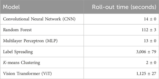
Table 5. Comparison of model roll-out time on the OLCI image in Figure 2. Times are rounded up to the nearest second. We display the mean and standard deviation across five different runs. Rolling-out with ViT is slow compared to the baseline models (with the exception of Label Spreading, which is slower).

Overall, the binned map in Figure 6 shows that ViTs, owing to their exceptional ability for detecting leads, have the potential to be used for automatically generating full lead products in the Arctic. Moreover, the segmentation maps in Figure 7 show that their performance is robust, detecting leads reliably even on OLCI images that were not used to build our labelled dataset for training the model (the original OLCI swaths are shown in Figure 8). Some issues remain however, including their high computational and memory cost for rolling out, and the fact that they have a tendency to label leads more generously than they should (see discussion in Section 4.3). In the future, we aim to refine our method further and develop a useable lead detection product by addressing these issues.

Figure 8

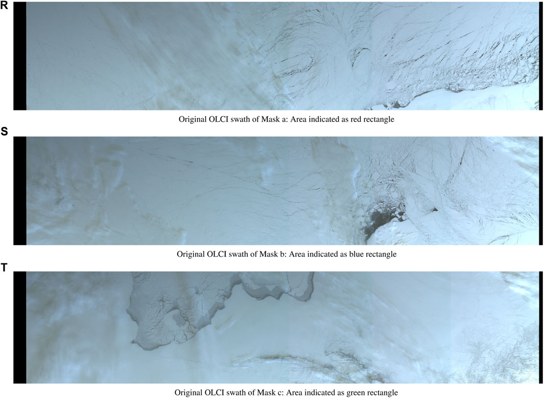
Figure 8. Original OLCI swaths indicated by the highlighted rectangles in Figure 6. Namely, regions (R) red rectangle, (S) blue rectangle, and (T) green rectangle.

5 Discussion

5.1 Discrepancy between accuracy metrics and roll-out performance

In our experiments, the Vision Transformer, while not achieving the highest test accuracy among all the models we evaluated, demonstrated the best roll-out performance qualitatively (and in comparison to the results produced by IRIS). This discrepancy leads us to ask why models such as Random Forest produce high test accuracy, despite it performing poorly on image roll-outs.

We believe that this is primarily due to the biases that are present in our curated dataset, arising from our labelling method and the initial data pre-processing. Thus, it is likely that models such as Random Forest and Label Spreading, which yield good test accuracy results, are fitting on the biases that exist in the dataset. One such bias comes from the Waveform Mixture Algorithm (WMA) used to produce the labels. Hence, a model that produces high accuracy on the labelled data can only accurately output what the WMA would have predicted, which itself is prone to errors.

This however, still does not explain why the ViT performs well since they were trained on the same dataset. While an advantage of ViT is that it is able to learn long-range correlations in an image unlike CNNs (which only consider local correlations), since we only use 3 × 3 image patches as inputs, it is hard to believe that it is exploiting this feature to produce the excellent results that we see. In fact, we have also considered using larger image patches of size 5 × 5, 11 × 11 and 33 × 33, however we found that none of these performed as well as the architecture with input size 3 × 3 that we ended up using. Thus, it would be interesting to identify, out of all the components that make up the ViT architecture, what is responsible for its ability to generalise well and not overfit on the bias in the dataset. Understanding this may help us to develop a neural network architecture specialised for our task that is cheaper to train or run, addressing also the computational cost issue that we discuss next in Section 5.2. On the other hand, we may also ask if improving the quality of the labelled dataset with smaller biases would result in improved roll-out performances using simpler, cheaper methods such as Random Forest.

5.2 Computational cost

According to the data presented in Table 5, the Vision Transformer (ViT) requires a significantly longer time for inference when processing the same dataset compared to other models. Indeed, transformer-based models are often slower than their counterparts, such as Convolutional Neural Networks (CNNs) (Wang et al., 2022). This decreased speed can be attributed to their extensive number of parameters and specific design features, such as the attention mechanism.

The extended processing time compromises the model’s scalability for analysing large datasets. For instance, achieving monthly lead detection becomes a formidable challenge. This limitation persists even when utilizing high-performance processors (GPUs), indicating that the model’s speed is a critical bottleneck for large-scale applications. In addition, longer processing times also suggest an issue of higher carbon costs.

Further advancements could be achieved by converting the model into a more compact version through techniques such as pruning and quantization. Emerging methodologies for pruning and quantization are applicable to deep learning models, including ResNet50, YOLOv5, and Bidirectional Encoder Representations from Transformers (BERT), as outlined by (Frantar and Alistarh, 2022). These methods can significantly reduce inference time while only minimally impacting model performance.

5.3 Surface contamination

The issue of various types of contamination and coverage, including land and cloud shadows, on the satellite footprint’s surface can potentially compromise image quality and, consequently, model performance. In our experiments, we primarily selected images with minimal cloud cover for training. However, completely avoiding cloud presence proved challenging.

During the roll-out, we observed that the Vision Transformer (ViT) model exhibits superior performance in disregarding (thin) cloud cover compared to other models. This discovery suggests potential paths for enhancing cloud mask creation and detection techniques.

5.4 Lead definition

According to the validation procedure implemented by IRIS, issues have been identified in the definition of leads, specifically concerning the differentiation between refrozen leads and open water leads. The classification provided by IRIS appears to be less inclusive compared to that of the Vision Transformer (ViT), which adopts a broader definition of leads, likely influenced by the labeling of its training data. The labels, derived from Synthetic Aperture Radar (SAR) imagery, may contain inaccuracies resulting from off-nadir contamination.

Further research could benefit from integrating high-resolution (HR) imagery, both optical and microwave, to more accurately delineate leads. Additionally, leveraging improved altimetry for lead classification and examining other characteristics of leads, such as thickness and type (e.g., refrozen), could offer deeper insights and improvements in understanding and detecting leads more accurately.

6 Conclusion

Understanding and tracking leads provides crucial insights into the broader dynamics of sea ice and its interactions with oceanic and atmospheric systems. Vision Transformers (ViTs), as a state-of-the-art algorithm for image classification, have shown promising results in addressing this issue. Our findings indicate that although ViTs do not achieve the best performance on the testing set, they can identify leads with greater sensitivity than other models, including CNNs, MLPs, K-Means clustering, Label Spreading, and Random Forests. This is particularly evident in scenarios where leads are not prevalent in ice-covered regions. Furthermore, ViTs have the potential to be used in creating a monthly lead product, provided that issues related to cloud contamination and lead definition can be more accurately addressed.

Data availability statement

The original contributions presented in the study are included in the article/supplementary material, further inquiries can be directed to the corresponding author. The code and example data can be found in the Github repo: https://github.com/totony4real/Vit-Sea-ice-and-lead-classifier.

Author contributions

WC: Writing–original draft, Writing–review and editing. MT: Writing–original draft, Writing–review and editing. RW: Writing–original draft, Writing–review and editing. ST: Writing–original draft, Writing–review and editing. DB: Writing–review and editing. CD: Writing–review and editing. AF: Writing–review and editing. TJ: Writing–review and editing. JL: Writing–review and editing. IL: Writing–review and editing. SL: Writing–review and editing. DN: Writing–review and editing. WL: Writing–review and editing. CN: Writing–review and editing. JS: Writing–review and editing. LH: Writing–review and editing. MD: Writing–review and editing.

Funding

The author(s) declare that financial support was received for the research, authorship, and/or publication of this article. WC and MT acknowledge support from ESA (Clev2er: CRISTAL LEVel-2 procEssor prototype and R&D); MT acknowledges support from (\#ESA/AO/1-9132/17/NL/MP, \#ESA/AO/1-10061/19/I-EF, SIN’XS: Sea Ice and Iceberg and Sea-ice Thickness Products Inter-comparison Exercise) and NERC (\#NE/T000546/1 761 \and \#NE/X004643/1). ST acknowledges support from a Department of Defense Vannevar Bush Faculty Fellowship held by Prof. Andrew Stuart, and by the SciAI Center, funded by the Office of Naval Research (ONR), under Grant Number N00014-23-1-2729. CN acknowledges support from NERC \#NE/S007229/1. RW and MT secured funding to initiate the study via the UCL MAPS Research Internship fund. RW and JS acknowledge funding from the NERC DEFIANT grant (\#NE/W004712/1), the European Union’s Horizon 2020 research and innovation programme via project CRiceS (grant no. 101003826) and European Space Agency NEOMI grant 4000139243/22/NL/SD. JS acknowledge funding from the Canada C150 grant 50296. JL acknowledges support from the INTERAAC project under Grant 328957 from the Research Council of Norway (RCN) and from the Fram Centre program for Sustainable Development of the Arctic Ocean (SUDARCO) under Grant 2551323.

Acknowledgments

MT and WC thank the UCL students of the module Artificial Intelligence for Earth Observation (AI4EO) promotion 2023/2024 who contributed to the IRIS surface classification shown in Figure 4.

Conflict of interest

The authors declare that the research was conducted in the absence of any commercial or financial relationships that could be construed as a potential conflict of interest.

Publisher’s note

All claims expressed in this article are solely those of the authors and do not necessarily represent those of their affiliated organizations, or those of the publisher, the editors and the reviewers. Any product that may be evaluated in this article, or claim that may be made by its manufacturer, is not guaranteed or endorsed by the publisher.

References

Asadi, N., Scott, K. A., Komarov, A. S., Buehner, M., and Clausi, D. A. (2020). Evaluation of a neural network with uncertainty for detection of ice and water in sar imagery. IEEE Trans. Geoscience Remote Sens. 59, 247–259. doi:10.1109/tgrs.2020.2992454

CrossRef Full Text | Google Scholar

Bij de Vaate, I., Martin, E., Slobbe, D. C., Naeije, M., and Verlaan, M. (2022). Lead detection in the arctic ocean from Sentinel-3 satellite data: a comprehensive assessment of thresholding and machine learning classification methods. Mar. Geod. 45, 462–495. doi:10.1080/01490419.2022.2089412

CrossRef Full Text | Google Scholar

Dawson, G., Landy, J., Tsamados, M., Komarov, A. S., Howell, S., Heorton, H., et al. (2022). A 10-year record of arctic summer sea ice freeboard from cryosat-2. Remote Sens. Environ. 268, 112744. doi:10.1016/j.rse.2021.112744

CrossRef Full Text | Google Scholar

Denton, A. A., and Timmermans, M.-L. (2022). Characterizing the sea-ice floe size distribution in the Canada basin from high-resolution optical satellite imagery. Cryosphere 16, 1563–1578. doi:10.5194/tc-16-1563-2022

CrossRef Full Text | Google Scholar

Donlon, C., Berruti, B., Buongiorno, A., Ferreira, M.-H., Féménias, P., Frerick, J., et al. (2012). The global monitoring for environment and security (gmes) Sentinel-3 mission. Remote Sens. Environ. 120, 37–57. doi:10.1016/j.rse.2011.07.024

CrossRef Full Text | Google Scholar

Dosovitskiy, A., Beyer, L., Kolesnikov, A., Weissenborn, D., Zhai, X., Unterthiner, T., et al. (2020). An image is worth 16x16 words: Transformers for image recognition at scale. arXiv preprint arXiv:2010.11929.

Google Scholar

ESA-PhiLab (2024). Iris - a toolbox for interferometric sar image reconstruction, analysis, and visualization. Available at: https://github.com/ESA-PhiLab/iris (Accessed February 26, 2024).

Google Scholar

European Space Agency (2011). CryoSat-2 product handbook. Available at: https://earth.esa.int/eogateway/documents/20142/37627/CryoSat-Baseline-D-Product-Handbook.pdf.

Google Scholar

European Space Agency (2022). Sentinel-3 SRAL land user handbook. Available at: https://sentinel.esa.int/documents/247904/4871083/Sentinel-3+SRAL+Land+User+Handbook+V1.1.pdf.

Google Scholar

Frantar, E., and Alistarh, D. (2022). Optimal brain compression: a framework for accurate post-training quantization and pruning. Adv. Neural Inf. Process. Syst. 35, 4475–4488. doi:10.48550/arXiv.2208.11580

CrossRef Full Text | Google Scholar

Guo, W., Itkin, P., Singha, S., Doulgeris, A. P., Johansson, M., and Spreen, G. (2022). Sea ice classification of terrasar-x scansar images for the mosaic expedition incorporating per-class incidence angle dependency of image texture. Cryosphere Discuss. doi:10.5194/tc-17-1279-2023

CrossRef Full Text | Google Scholar

Han, Y., Liu, Y., Hong, Z., Zhang, Y., Yang, S., and Wang, J. (2021). Sea ice image classification based on heterogeneous data fusion and deep learning. Remote Sens. 13, 592. doi:10.3390/rs13040592

CrossRef Full Text | Google Scholar

Heorton, H. D., Tsamados, M., Cole, S., Ferreira, A. M., Berbellini, A., Fox, M., et al. (2019). Retrieving sea ice drag coefficients and turning angles from in situ and satellite observations using an inverse modeling framework. J. Geophys. Res. Oceans 124, 6388–6413. doi:10.1029/2018jc014881

CrossRef Full Text | Google Scholar

Ho, T. K. (1995). Random decision forests. Proc. 3rd Int. Conf. document analysis Recognit. (IEEE) 1, 278–282.

Google Scholar

Hoffman, J. P., Ackerman, S. A., Liu, Y., and Key, J. R. (2019). The detection and characterization of arctic sea ice leads with satellite imagers. Remote Sens. 11, 521. doi:10.3390/rs11050521

CrossRef Full Text | Google Scholar

Hoffman, J. P., Ackerman, S. A., Liu, Y., Key, J. R., and McConnell, I. L. (2021). Application of a convolutional neural network for the detection of sea ice leads. Remote Sens. 13, 4571. doi:10.3390/rs13224571

CrossRef Full Text | Google Scholar

Horvat, C., Buckley, E., Stewart, M., Yoosiri, P., and Wilhelmus, M. M. (2023). Linear ice fraction: sea ice concentration estimates from the icesat-2 laser altimeter. EGUsphere 2023, 1–18. doi:10.5194/egusphere-2023-2312

CrossRef Full Text | Google Scholar

Horvat, C., Roach, L. A., Tilling, R., Bitz, C. M., Fox-Kemper, B., Guider, C., et al. (2019). Estimating the sea ice floe size distribution using satellite altimetry: theory, climatology, and model comparison. Cryosphere 13, 2869–2885. doi:10.5194/tc-13-2869-2019

CrossRef Full Text | Google Scholar

Huang, Y., Ren, Y., and Li, X. (2024). Deep learning techniques for enhanced sea-ice types classification in the beaufort sea via sar imagery. Remote Sens. Environ. 308, 114204. doi:10.1016/j.rse.2024.114204

CrossRef Full Text | Google Scholar

Hutter, N., and Losch, M. (2020). Feature-based comparison of sea ice deformation in lead-permitting sea ice simulations. Cryosphere 14, 93–113. doi:10.5194/tc-14-93-2020

CrossRef Full Text | Google Scholar

Kacimi, S., and Kwok, R. (2021). Three years of snow depth and ice thickness from icesat-2 and cryosat-2. AGU Fall Meet. Abstr. 2021.

Google Scholar

Kaleschke, L., Richter, A., Burrows, J., Afe, O., Heygster, G., Notholt, J., et al. (2004). Frost flowers on sea ice as a source of sea salt and their influence on tropospheric halogen chemistry. Geophys. Res. Lett. 31. doi:10.1029/2004gl020655

CrossRef Full Text | Google Scholar

Kern, S., Lavergne, T., Notz, D., Pedersen, L. T., Tonboe, R. T., Saldo, R., et al. (2019). Satellite passive microwave sea-ice concentration data set intercomparison: closed ice and ship-based observations. Cryosphere 13, 3261–3307. doi:10.5194/tc-13-3261-2019

CrossRef Full Text | Google Scholar

Khaleghian, S., Ullah, H., Kræmer, T., Eltoft, T., and Marinoni, A. (2021). Deep semisupervised teacher–student model based on label propagation for sea ice classification. IEEE J. Sel. Top. Appl. Earth Observations Remote Sens. 14, 10761–10772. doi:10.1109/jstars.2021.3119485

CrossRef Full Text | Google Scholar

Koo, Y., Xie, H., Kurtz, N. T., Ackley, S. F., and Wang, W. (2023). Sea ice surface type classification of icesat-2 atl07 data by using data-driven machine learning model: ross sea, antarctic as an example. Remote Sens. Environ. 296, 113726. doi:10.1016/j.rse.2023.113726

CrossRef Full Text | Google Scholar

Kwok, R. (2018). Arctic sea ice thickness, volume, and multiyear ice coverage: losses and coupled variability (1958–2018). Environ. Res. Lett. 13, 105005. doi:10.1088/1748-9326/aae3ec

CrossRef Full Text | Google Scholar

Landy, J. C., Dawson, G. J., Tsamados, M., Bushuk, M., Stroeve, J. C., Howell, S. E., et al. (2022). A year-round satellite sea-ice thickness record from cryosat-2. Nature 609, 517–522. doi:10.1038/s41586-022-05058-5

PubMed Abstract | CrossRef Full Text | Google Scholar

Laxon, S., Peacock, H., and Smith, D. (2003). High interannual variability of sea ice thickness in the arctic region. Nat. 2003 425, 947–950. doi:10.1038/nature02050

PubMed Abstract | CrossRef Full Text | Google Scholar

LeCun, Y., and Bengio, Y. (1995). Convolutional networks for images, speech, and time series. Handb. brain theory neural Netw. 3361, 1995.

Google Scholar

Lee, S., Kim, H.-c., and Im, J. (2018). Arctic lead detection using a waveform mixture algorithm from cryosat-2 data. Cryosphere 12, 1665–1679. doi:10.5194/tc-12-1665-2018

CrossRef Full Text | Google Scholar

Liang, Z., Pang, X., Ji, Q., Zhao, X., Li, G., and Chen, Y. (2022). An entropy-weighted network for polar sea ice open lead detection from Sentinel-1 sar images. IEEE Trans. Geoscience Remote Sens. 60, 1–14. doi:10.1109/tgrs.2022.3169892

CrossRef Full Text | Google Scholar

Lindsay, R., and Schweiger, A. (2015). Arctic sea ice thickness loss determined using subsurface, aircraft, and satellite observations. Cryosphere 9, 269–283. doi:10.5194/tc-9-269-2015

CrossRef Full Text | Google Scholar

Lüpkes, C., Vihma, T., Birnbaum, G., and Wacker, U. (2008). Influence of leads in sea ice on the temperature of the atmospheric boundary layer during polar night. Geophys. Res. Lett. 35. doi:10.1029/2007gl032461

CrossRef Full Text | Google Scholar

MacQueen, J. (1967). Some methods for classification and analysis of multivariate observations. Proc. fifth Berkeley symposium Math. statistics Probab. 1, 281–297.

Google Scholar

Marcq, S., and Weiss, J. (2012). Influence of sea ice lead-width distribution on turbulent heat transfer between the ocean and the atmosphere. Cryosphere 6, 143–156. doi:10.5194/tc-6-143-2012

CrossRef Full Text | Google Scholar

Massom, R. A. (1988). The biological significance of open water within the sea ice covers of the polar regions. Endeavour 12, 21–27. doi:10.1016/0160-9327(88)90206-2

CrossRef Full Text | Google Scholar

Muchow, M., Schmitt, A. U., and Kaleschke, L. (2021). A lead-width distribution for antarctic sea ice: a case study for the weddell sea with high-resolution Sentinel-2 images. cryosphere 15, 4527–4537. doi:10.5194/tc-15-4527-2021

CrossRef Full Text | Google Scholar

Mugunthan, J. S. (2023). Evaluation of machine learning algorithms for the classification of lake ice and open water from Sentinel-3 sar altimetry waveforms. UWSpace.

Google Scholar

Murtagh, F. (1991). Multilayer perceptrons for classification and regression. Neurocomputing 2, 183–197. doi:10.1016/0925-2312(91)90023-5

CrossRef Full Text | Google Scholar

NASA (2023). Snap data processors - radiance-to-reflectance conversion algorithm specification.

Google Scholar

Ólason, E., Rampal, P., and Dansereau, V. (2021). On the statistical properties of sea-ice lead fraction and heat fluxes in the arctic. Cryosphere 15, 1053–1064. doi:10.5194/tc-15-1053-2021

CrossRef Full Text | Google Scholar

Perovich, D., Grenfell, T., Light, B., and Hobbs, P. (2002). Seasonal evolution of the albedo of multiyear arctic sea ice. J. Geophys. Res. Oceans 107, SHE–20. doi:10.1029/2000jc000438

CrossRef Full Text | Google Scholar

Petty, A. A., Bagnardi, M., Kurtz, N., Tilling, R., Fons, S., Armitage, T., et al. (2021). Assessment of icesat-2 sea ice surface classification with Sentinel-2 imagery: implications for freeboard and new estimates of lead and floe geometry. Earth Space Sci. 8, e2020EA001491. doi:10.1029/2020ea001491

CrossRef Full Text | Google Scholar

Qiu, Y., Li, X.-M., and Guo, H. (2023). Spaceborne thermal infrared observations of arctic sea ice leads at 30 m resolution. EGUsphere, 1–33.

Google Scholar

Qu, M., Pang, X., Zhao, X., Lei, R., Ji, Q., Liu, Y., et al. (2021). Spring leads in the beaufort sea and its interannual trend using terra/modis thermal imagery. Remote Sens. Environ. 256, 112342. doi:10.1016/j.rse.2021.112342

CrossRef Full Text | Google Scholar

Quartly, G. D., Rinne, E., Passaro, M., Andersen, O. B., Dinardo, S., Fleury, S., et al. (2019). Retrieving sea level and freeboard in the arctic: a review of current radar altimetry methodologies and future perspectives. Remote Sens. 11, 881. doi:10.3390/rs11070881

CrossRef Full Text | Google Scholar

Reiser, F., Willmes, S., and Heinemann, G. (2020). A new algorithm for daily sea ice lead identification in the arctic and antarctic winter from thermal-infrared satellite imagery. Remote Sens. 12, 1957. doi:10.3390/rs12121957

CrossRef Full Text | Google Scholar

Ren, Y., Li, X., Yang, X., and Xu, H. (2021). Development of a dual-attention u-net model for sea ice and open water classification on sar images. IEEE Geoscience Remote Sens. Lett. 19, 1–5. doi:10.1109/lgrs.2021.3058049

CrossRef Full Text | Google Scholar

Stroeve, J., and Notz, D. (2018). Changing state of arctic sea ice across all seasons. Environ. Res. Lett. 13, 103001. doi:10.1088/1748-9326/aade56

CrossRef Full Text | Google Scholar

Vaswani, A., Shazeer, N., Parmar, N., Uszkoreit, J., Jones, L., Gomez, A. N., et al. (2017). Attention is all you need. Adv. neural Inf. Process. Syst. 30. doi:10.48550/arXiv.1706.03762

CrossRef Full Text | Google Scholar

von Albedyll, L., Hendricks, S., Hutter, N., Murashkin, D., Kaleschke, L., Willmes, S., et al. (2023). Lead fractions from sar-derived sea ice divergence during mosaic. Cryosphere Discuss. 2023, 1–39. doi:10.5194/tc-18-1259-2024

CrossRef Full Text | Google Scholar

Wang, X., Zhang, L. L., Wang, Y., and Yang, M. (2022). “Towards efficient vision transformer inference: a first study of transformers on mobile devices,” in Proceedings of the 23rd Annual International Workshop on Mobile Computing Systems and Applications, Toronto, ON, Canada, 1–7.

Google Scholar

Wernecke, A., and Kaleschke, L. (2015). Lead detection in arctic sea ice from cryosat-2: quality assessment, lead area fraction and width distribution. Cryosphere 9, 1955–1968. doi:10.5194/tc-9-1955-2015

CrossRef Full Text | Google Scholar

Wilchinsky, A. V., Heorton, H. D., Feltham, D. L., and Holland, P. R. (2015). Study of the impact of ice formation in leads upon the sea ice pack mass balance using a new frazil and grease ice parameterization. J. Phys. Oceanogr. 45, 2025–2047. doi:10.1175/jpo-d-14-0184.1

CrossRef Full Text | Google Scholar

Willmes, S., and Heinemann, G. (2015a). Pan-arctic lead detection from modis thermal infrared imagery. Ann. Glaciol. 56, 29–37. doi:10.3189/2015aog69a615

CrossRef Full Text | Google Scholar

Willmes, S., and Heinemann, G. (2015b). Sea-ice wintertime lead frequencies and regional characteristics in the arctic, 2003–2015. Remote Sens. 8, 4. doi:10.3390/rs8010004

CrossRef Full Text | Google Scholar

Zhou, D., Yu, Z., Xie, E., Xiao, C., Anandkumar, A., Feng, J., et al. (2022). “Understanding the robustness in vision transformers,” in International Conference on Machine Learning (PMLR), Honolulu, United States, 23-29 July 2023, 27378–27394.

Google Scholar

Zhu, X., and Ghahramani, Z. (2002). Learning from labeled and unlabeled data with label propagation. Pennsylvania, United States: Carnegie Mellon University. Technical Report. CMU-CALD-02-106.

Google Scholar