 Mikhail D. Alexandrov
 Brian Cairns
 Claudia Emde
 Bastiaan Van Diedenhoven
- 1Department of Applied Physics and Applied Mathematics, Columbia University, New York, NY, United States
- 2NASA Goddard Institute for Space Studies, New York, NY, United States
- 3Meteorologisches Institut, Ludwig-Maximilians-Universitat, Munich, Germany
- 4Deutsches Zentrum fur Luft- und Raumfahrt, Institut fur Physik der Atmosphare, Oberpfaffenhofen, Germany
- 5SRON Netherlands Institute for Space Research, Leiden, Netherlands
3D effects cause substantial underestimation of cloud optical thickness (COT) in airborne and satellite retrievals based on 1D radiative transfer computations (such as in the case of widely used bispectral technique). For a single-layer isolated cloud we propose a simple linear correction of the retrieved COT with the renormalization factor dependent on the cloud’s aspect ratio (the ratio between vertical and horizontal dimensions of the cloud). This is an empirical assumption which we successfully test using synthetic 3D RT data. We introduce a heuristic “block model” of 3D radiative effects and show that the functional form of the renormalization factor is consistent with the process of radiation escape from cloud sides in an essentially 3D geometry. We also extend the block model to the case of single-layer broken cloud field with radiative interaction between the neighboring clouds. In this case the renormalization factor depends also on the distance between clouds.
1 Introduction
Currently operational algorithms for satellite retrievals of cloud optical thickness (COT) and droplet size are based on bispectral measurements in absorbing and non-absorbing bands (Nakajima and King, 1990). Such algorithms are used, e.g., to generate data products based on the Moderate Resolution Imaging Spectroradiometer (MODIS) measurements (Platnick et al., 2003). Similar algorithm (along with its modified version relying on cloud droplet size derived from polarized reflectances) is also applied to measurements made by the airborne Research Scanning Polarimeter (RSP). These retrieval techniques have certain limitations owing to the influence of 3D structure of clouds (especially broken) on the reflected solar radiation, which is not accounted for in the look-up tables (LUTs) based on 1D radiative transfer models (Marshak et al., 2006; Zinner et al., 2010). The satellite data survey by Di Girolamo et al. (2010) found that the retrieved cloud reflectance is consistent with plane-parallel RT model only in 24% of cases, mostly limited to regions dominated by stratiform clouds at solar zenith angles less than 60° (for other regions or solar angles this frequency drops sharply to as low as a few percent). 3D radiative effects, such as escape of light through cloud sides and shadowing, can cause substantial underestimation of COT by 1D-RT-based retrieval techniques. Zhang and Platnick (2011) also reported significant overestimation of droplet size by the MODIS bispectral algorithm.
Correct COT is also important because of its role in calibration of the extinction coefficient fields computed using the tomographic technique designed by Alexandrov et al. (2021). The subjects of tomographic retrievals are isolated clouds such as Cu or CuCg (Tcu), which radiative properties are significantly impacted by 3D effects.
In this study (Part I of the series) we introduce the concept of linear correction of COTs of single-layer clouds retrieved using LUT based on 1D RT computations. This correction is simply multiplication of COT value by a renormalization factor depending on the cloud aspect ratio. We also present validation of this correction method based on 3D RT simulations. And finally, we provide theoretical justification of our technique based on a simple geometrical model, which allows for estimation of the effect of radiation escape through cloud sides on the cloud-top reflectance and subsequently on COT retrievals. We also extend this model designed for isolated cloud case to that for broken cloud field. In the upcoming Part II of the series we will present a comprehensive COT renormalization theory accounting for the relationship between reflectance and COT. We will also derive correction factors for essentially 3D (close to isotropic) scattering.
2 Motivation: renormalization of inhomogeneous COT
Cairns et al. (2000) suggested a renormalization of cloud optical properties allowing to use plane-parallel computations in the case of non-homogeneous cloud with horizontally varying droplet number concentration
Here
in plane-parallel computations. Here
is the relative variance of the droplet number concentration, which is an effective measure of the inhomogeneity of the actual cloud field. Equation 2 shows that in order to mimic cloud inhomogeneity effects in plane parallel computations the value of σext should be decreased by the factor 1 + V. This results in smaller reflectances compared to those computed with the actual σext.
While derived for simplification of forward RT computations in general circulation models (GCM), this result can be adopted for use in cloud remote sensing. The retrieval of the extinction in an inhomogeneous cloud using a LUT based on plane-parallel computations yields the value of
In the context of airborne and satellite remote sensing the primary measured quantity is COT τ (rather than Nc, which is a more advanced data product (Grosvenor et al., 2018)). Thus, it is convenient to replace Eqs 2, 3 with
and
respectively (angular brackets denote the ensemble averaging). Here we denote by τmeas the COT retrieved from the measurements using a technique based on 1D RT (e.g., bispectral), while τren is the “true” (renormalized) COT value. Note that since (1 + V) is a constant factor, the value of V can be computed using the measured COT τmeas in Eq. 5 instead of the actual τren. Note that V is closely related to the reflectance-based inhomogeneity parameter
the correction factor in Eq. 4 can be written as
3 Renormalization of isolated cloud’s COT
The COT retrievals for isolated clouds are affected by 3D effects that are caused by their geometry, such as light escape from cloud sides that decreases the reflectance at cloud top and leads to underestimation of the COT. Results for the path length statistics of random walks (Blanco and Fournier, 2006) and for the searchlight problem for a 1D cloud (Marshak et al., 1995) suggest that the aspect ratio of the scattering object plays a key role in controlling the path length statistics and the loss of radiation through cloud sides. In the case of clouds, scattering of light by large cloud droplets is strongly forward-directed with radiation staying close to the solar principal plane for clouds that are not too optically thick. In this case the radiative transfer can be assumed to be close to two-dimensional.
2D shape of a single-layer cloud is characterized by the cloud’s vertical and horizontal dimensions
respectively. Here h and x are vertical and horizontal coordinates of the points at the cloud’s “boundary”. This definition is applicable to any cloud shape. Then the cloud’s aspect ratio is defined as
Motivated by the results presented in Section 2 we suggest to correct the isolated cloud’s COT using the factor similar to that in Eq. 4 but with the variability parameter V replaced by the cloud’s aspect ratio A:
The larger is A, the more radiation passes through it’s sides causing larger negative bias in τmeas. On the other hand, a plane-parallel cloud has L → ∞ and A = 0, so the correction factor equals to unity (i.e., τren = τmeas). Physical explanation of this model is provided in Section 5 below.
4 Tests on simulated data
In order to test the above proposition, we performed COT retrievals from simulated reflectances using the operational retrieval algorithm designed for the RSP data analysis (Alexandrov et al., 2012). This algorithm uses nadir-view reflectances and is a modification of the legacy bispectral technique (Nakajima and King, 1990). In the modified version the droplet effective radius is retrieved from the polarized reflectance at 863-nm wavelength and no absorbing spectral channels are used. For the simulated datasets we imply that the reff is known and take its value (12 μm) from the cloud model to which the 3D RT computations were applied. Note that we use 863-nm LUT to retrieve COT values while the simulations described below are made at 555-nm wavelength. However, this should not have any noticeable effect on the retrievals since COT in this spectral range is almost wavelength-independent.
The simulations of the RSP measurements were produced by the 3D radiative transfer model MYSTIC (Monte Carlo code for the phYSically correct Tracing of photons In Cloudy atmospheres (Mayer, 2009; Emde et al., 2010)). Two different types of simulations were used: a smaller dataset based on clouds generated using Large Eddies Simulations (LES) and a more extensive dataset based on simplified box clouds with prescribed aspect ratios and COTs.
4.1 Simulations based on LES-generated clouds
The simulations presented in this section have been already used in our previous work (Alexandrov et al., 2010; Alexandrov et al., 2012; Alexandrov et al., 2016; Alexandrov et al., 2021). These are the results of 3D RT computations applied to LES-generated realistic maritime Cu cloud field (Ackerman et al., 2004). The simulated RSP measurements were produced assuming that the instrument is flown in the solar principal plane at 2.4 km altitude. The assumed solar zenith angle is 40°, the surface albedo is 5%, and the measurement wavelength is 555 nm. The RSP measurements were simulated on the grid with 100 m spacing.
As it would be in the case of real field experiment, we estimate the cloud aspect ratios from the remote sensing data: they are derived from cloud shapes obtained using cut-out (“space curving”) technique (Alexandrov et al., 2016; Alexandrov et al., 2021) applied to the simulated RSP measurements. These shapes for three clouds in the simulated dataset are shown in Figure 1 (left) (reproduced from Alexandrov et al. (2016)). While they depend on the threshold in total reflectance, the aspect ratios appear to be not very sensitive to the threshold value. Each plot in Figure 1 (left) shows two shapes corresponding to different thresholds (in white for the smaller one, in black for the larger) with the corresponding aspect ratios A1 and A2 respectively (computed according to Eqs 8, 9. Blue curves in Figure 1 (right) depict the COTs computed based on extinction coefficient fields from the respective LES outputs (Alexandrov et al., 2021). Solid red curves in these plots correspond to COT retrievals made using the RSP algorithm described above. The RSP-derived COT values appear to be notably smaller than their LES counterparts. Note that τRSP curves are shifted towards the bright sides of the clouds (to the left in our case) relative to the radiation-independent τLES. The dashed red curves depict the τRSP “corrected” by multiplication by the corresponding matching factors
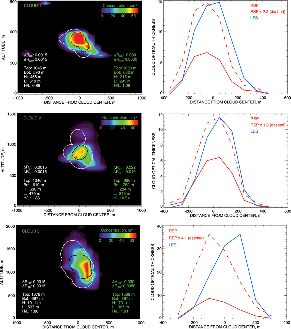
Figure 1. Left: Cloud shapes derived using the remote sensing technique applied to simulated data for two different reflectance thresholds plotted over the droplet number concentration fields taken from LES datasets. The plots are reproduced from Alexandrov et al. (2016). Right: Comparison between the COT retrieved from virtual RSP data (red) and the actual one computed from the LES data (blue). The dashed red curve depicts the retrieved COT scaled to match the maximum of the actual COT (see Eq. 11).
The renormalization factors (1 + A1) and (1 + A2) corresponding to the two shapes in each plot in Figure 1 (left) are presented in Table 1 in comparison with the COT matching factor χ from Figure 1 (right). For the first two clouds the relation 1 + A ≈ χ holds quite well, especially for A2: 2.1 vs. 2.2 and 1.9 vs. 1.8 respectively. For Cloud three the deviation between the renormalization and matching factors is larger: 2.9 vs. 4.1, while the correction of such magnitude is still very valuable. The difference between the first two and the last cloud cases can be explained by the differences in their COT: Cloud three is much thicker optically (τLES ≈ 35 at maximum vs. 15 and 12 for Couds one and two respectively). This may be a result of saturation of COT retrievals in the bispectral algorithm at larger values of the reflectances, or the breakdown of the assumed 2D transport of radiation through the cloud at high optical depths, so that an additional correction that is dependent on τRSP may be needed.
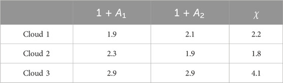
Table 1. Comparison between the renormalization factors (1 + A) based on the aspect ratios from Figure 1 (left) and the actual matching factors χ (Eq. 11) from Figure 1 (right).
It is important to note that the three clouds in our LES-generated examples have different shapes, internal structures and microphysics. They are inhomogeneous both vertically and horizontally. However, in all three cases the COT retrieval errors agree well with Eq. 10. This means that while radiative transfer in clouds is a complicated process governed by many cloud parameters, the cloud aspect ratio appears to be the dominant factor characterizing the influence of 3D effects on COT retrievals.
4.2 Simulations based on box clouds
Box clouds used in these simulations were L × L × H single-layer cuboids with the virtual RSP flying at 6,000 m altitude over their centers in solar principle plane parallel to the clouds horizontal edges. The solar zenith angle was 60°, surface albedo was 5%, and the RSP measurements were made every 100 m at 555-nm wavelength. We used gamma droplet size distribution with the effective radius of 12 μm and effective variance of 0.1. The light scattering in this model is essentially two-dimensional, so the clouds can be represented by L × H rectangles. The cloud horizontal dimension and cloud top height were the same for all clouds: L = 1,000 m and Htop = 4,000 m respectively, while we took four different values for cloud vertical dimension H: 500, 1,000, 2000, and 3,000 m. These cloud geometric thicknesses correspond to the aspect ratios A = 0.5, 1.0, 2.0, and 3.0 respectively. For each aspect ratio, clouds were simulated with three different values of COT: 10, 25, and 50, so our box-cloud dataset includes the total of 12 samples.
The geometries of two clouds from the dataset used in this study are presented in Figure 2 (left): one with the aspect ratio A = 0.5 (top) and the other with A = 3.0 (bottom). The corresponding model and retrieved COTs are presented in Figure 2 (right) as functions of the distance from the cloud center. The model COTs (25 in both cases) are shown in green while the ones retrieved using the RSP algorithm are plotted in blue. Note that both retrieved COT curves are skewed to the left toward the bright side of the cloud (more pronounced for the smaller A = 0.5) (cf. Alexandrov et al., 2021). As in the LES cloud case presented above, the RSP retrievals in Figure 2 (right) significantly underestimate the model COT values. It is also clear that the renormalization by the factor (1 + A) described in Section 3 (represented by red curves) notably improves the retrieval-model agreement.

Figure 2. Left: Cloud shapes and positions used in 3D RT simulations for box clouds with the aspect ratios A = 0.5 (top) and A = 3.0 (bottom). Right: the corresponding COT retrieved made using the RSP algorithm (blue), RSP COT renormalized by the factor (1 + A) (red), and the model COT = 25 (green).
For statistical comparisons we consider the maxima of the retrieved COT curves as the representative values for estimation of the retrieval accuracy. Plots in Figure 3 compare the initial (left) and renormalized (right) retrieved COTs with the corresponding model values. The colors of the data points in the scatter plots are associated with different cloud aspect ratios. It is clearly seen in the left panel that the errors of COT retrievals increase with A, while in the right panel the multiplication by (1 + A) moves the data points much closer to 1-1 line. Some small underestimation remains, which is almost negligible for τmod = 10 (bias of 0.5 ± 0.6) and τmod = 25 (bias of 1 ± 3), while somewhat larger for τmod = 50 (bias of 9 ± 3). These comparisons support the renormalization concept introduced in Section 3.
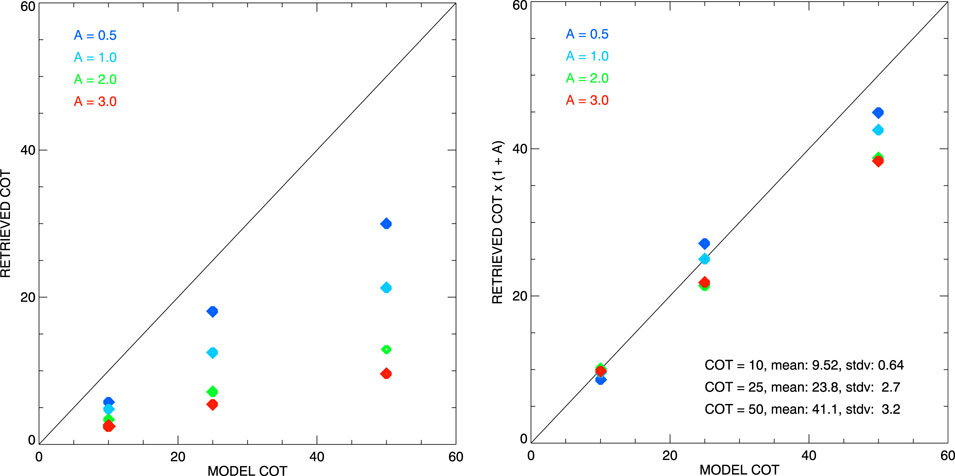
Figure 3. Scatter plots comparing model and retrieved (at maximum) COTs for box cloud simulations. Left: initial RSP-retrieved COTs. Right: retrieved COTs renormalized by the corresponding factors (A + 1).
5 Block model for radiation escape
The appearance of the factor (1 + A) in Eq. 10 can be justified using a very crude geometrical model illustrated in Figure 4. We will call it “Block Model” or BM. This is not a radiative transfer model but rather a geometrical “supplement” to 1D RT model allowing for account of 2D/3D radiative effects. In the 2D variant of this model clouds are assumed to be rectangular L × H homogeneous columns, with plane-parallel case corresponding to L → ∞. In the 3D variant clouds are rectangular parallelepipeds (cuboids). We do not specify neither the microphysical optical properties of the droplets within the cloud, nor how the incident flux Iin gets into it. There is no absorption in the model, so the total outgoing flux Iout is equal to Iin and the total cloud albedo is
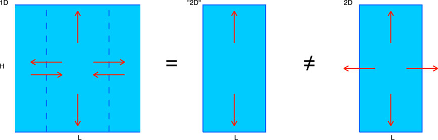
Figure 4. Schematic illustration of the renormalization setup discussed in Section 3. The radiative fluxes within an isolated cloud (blue) are depicted by red arrows in 1D (plane-parallel) case (left), in “equivalent” 2D case (middle) and in actual 2D case (right). The L × H virtual “subcloud” in 1D case is singled out by vertical dashed lines.
The main assumption of this model is that outgoing radiation is uniformly distributed along the cloud’s surface. Then the reflectance per unit boundary length/area is
where S is the total perimeter/surface of the cloud. This is the quantity that is measured by a narrow-view nadir-looking sensor located above the cloud.
Due to radiation escape through the cloud’s sides, the measured reflectance Rmeas = R is smaller than that from the infinite slab with the same COT. Thus, the COT τmeas derived from Rmeas using 1D-RT LUT will be also smaller than the actual one. This means that in order to facilitate accurate COT retrievals, Rmeas should be appropriately increased, so that its renormalized value
can be used in 1D-RT-based retrieval algorithm. Here κ ≥ 1 is the renormalization factor.
While no RT computations are performed within Block Model, it allows for estimation of the factor κ by comparison of radiation fluxes escaping the cloud in 1D (plane-parallel) and in 2D/3D cases:
Here R is the cloud-top reflectance Eq. 13 “measured” above the actual 2D/3D cloud and R1D is the one that would be measured if the cloud (with the same COT) was plane-parallel.
It is important to note that (unlike Eq. 10) and Eq. 14 relates reflectances, not COTs. It converts into
at small values of τ and R, when they are roughly proportional to each other. We will show in Part II in the framework of general renormalization theory that Eq. 16 is indeed valid for all COT values and should be used instead of Eq. 14.
6 Application of block model to 2D scattering
As we mentioned above, scattering of light by large cloud droplets is strongly forward directed with radiation staying close to the solar principal plane for clouds that are not too optically thick meaning that the transport of radiation is close to two-dimensional. In this section we will show that the correction factor (1 + A) in Eq. 10, which was validated using 3D RT simulations, can be derived from a simple heuristic 2D geometrical model. We then extend this model (initially designed for isolated cloud) to the case of broken cloud field where neighboring clouds radiatively interact with each other. The case of 3D scattering (close to isotropic) will be presented in Part II of this series. All clouds are assumed to be single-layer so there is no radiative interaction between cloud layers in vertical dimension.
6.1 Isolated cloud
We compare the cloud-top reflectances of two clouds with the same COT and vertical dimension H: horizontally infinite slab and L × H column. The former reflectance is determined by a 1D RT model, while the latter is influenced by 2D radiative effects. Let us single out a virtual L × H subset of the infinite cloud. Due to the symmetry, the same radiation fluxes enter this subset through the two its virtual vertical boundaries as exit through them (see Figure 4 (left)). Thus, the radiation field produced by this “subcloud” is equivalent to that of an actual L × H column but with totally reflective (mirror) vertical boundaries (Figure 4 (middle)). On the other hand, the finite cloud (Figure 4 (right)) has all its boundaries open for outgoing radiation. Note that these two clouds have the same dimensions, thus, their incoming radiation fluxes are the same.
In the mirror-walled cloud light can escape only through its top and bottom, so according to Eq. 13 with S = 2L the reflectance per unit boundary length for it is
while in the actual L × H cloud light escapes through its whole perimeter (S = 2L + 2H in Eq. 13), so in this case R = R2D has the following form
It can be written as
thus, the correction factor κ = κ2D defined by Eq. 15 is
Combining Eq. 20 with Eq. 16 yields Eq. 10. Note that in the limit case of wide cloud (L ≫ H) the aspect ratio A in Eq. 20 vanishes resulting in κ2D = 1, which indicates that no renormalization is necessary.
6.2 Broken cloud field
Let us consider an array of L × H clouds separated by gaps of the length D (Figure 5). This setting is a generalization of both infinite cloud and isolated cloud cases, which correspond to the limits of D = 0 and D → ∞ respectively. As it was described in the previous subsection, in the case of infinite cloud the vertical boundaries of a L × H virtual subcloud can be considered as mirrors reflecting all radiation attempting to escape through them (due to symmetry). When gaps are introduced between these virtual subclouds (which after this become actual clouds) some radiation starts to escape through the gaps’ vertical boundaries. The symmetry condition still holds for the part of radiation flux reaching the neighboring cloud (which can be then considered as returning to the initial cloud), while the part escaping through the top and bottom of the gap is lost permanently (see Figure 5 for a schematic illustration). The magnitude of this lost flux depends on the gap size D.
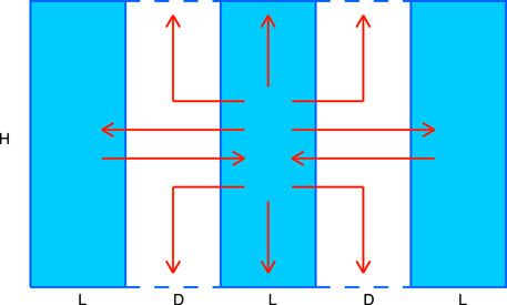
Figure 5. Schematic representation of broken cloud field setup in the case of 2D scattering. Red arrows depict the radiative fluxes leaving and entering the cloud in the middle.
The renormalization coefficient for the broken cloud field is derived in Supplementary Appendix SA1:
It has the same functional form as that for isolated cloud (Eq. 20) but with
being the analog of the cloud aspect ratio for 2D broken cloud field. Here Ag is the gap aspect ratio
Note that in Supplementary Appendix SA1 this expression also contains a constant factor which serves as a free parameter in the Block Model. Here we omit it for simplicity and clarity.
Equation 22 allows us to define the condition when the cloud can be considered isolated, i.e., when its radiative interaction with its neighbors is negligible. In this case A′ ≈ A corresponding to Ag ≪ 1 which can be neglected in the denominator of Eq. 22. This condition can be written as D ≫ H, meaning that the distances between clouds in the field substantially exceed clouds’ vertical dimensions. Completely isolated cloud corresponds to D → ∞. In this case Ag = 0 and A′ = A transforming Eq. 21 into Eq. 20. In the opposite case of D = 0 (infinite plane-parallel cloud) Ag → ∞ and A′ = 0 leaving κ2D = 1 (meaning that no renormalization is necessary).
Parameter Ag can be expressed in terms of the cloud aspect ratio A and the cloud fraction
as
where we introduced the coefficient
depending only on cloud fraction. In this terms
7 Discussion
Currently global COT datasets are derived from the single-angle measurements made by satellite-based imagers (such as MODIS, VIIRS, and OCI) using look-up tables based on 1D RT computations. Our 3D RT simulations presented in this paper showed that such inversions can underestimate COT by a factor of four (or possibly higher) due to presence 3D radiative effects (primarily radiation escape from the cloud’s sides) unaccounted for in 1D RT. This is the case for isolated clouds and for those in broken cloud fields. Such large bias in COT retrievals puts their value in question and may impair assessments of cloud effects on climate. Thus, finding a way for estimation of the biases and subsequent correction of the COT retrievals is a matter of the utmost importance.
This paper is Part I of the series targeting correction of airborne and satellite COT retrievals. In this study we introduced a correction (renormalization) procedure Eq. 10 for single-layer isolated cloud that is simply multiplication of the COT retrieved using LUT based on 1D RT by the factor (1 + A), where A is the cloud’s aspect ratio (the ratio between its vertical and horizontal dimensions). Then this assumption was successfully tested on two sets of 3D RT simulations: one based on three LES-generated marine Cu clouds (Figure 1) and the other using 12 simplified box clouds with prescribed COTs and aspect ratios (two of them presented in Figure 2). The COT retrievals in both cases were made from the measurements of nadir reflectances made by simulated Research Scanning Polarimeter (RSP) using the operational algorithm designed for the real instrument. The results of these computations presented in Table 1 and especially in Figure 3 demonstrate that the factor (1 + A) is an accurate estimate of the COT retrieval bias and can be successfully used for correction of the COT values derived based on 1D-RT LUTs.
Initially the factor (1 + A) was postulated by analogy with Eq. 4 derived to account for cloud inhomgeneity in COT retrievals. However, we then justified this choice using a heuristic geometrical model (Block Model) describing radiation escape from isolated cloud in comparison with that from infinite plane-parallel cloud (see Figure 4). This model was subsequently extended to the case of broken cloud field in the presence of radiative interaction between neighboring clouds (Figure 5). The resulting correction factor is defined by Eqs 21–23. This expression still needs to be validated using 3D RT simulations. In near future we plan to perform such simulations using a set of box-cloud fields with different characteristics. The results will be reported in our subsequent publications.
A more detailed theoretical basis of COT renormalization will be presented in upcoming Part II of the series resolving some issues left unaddressed in this study. In particular, we will introduce generalized renormalization theory and explain why the correction factors derived in the Block Model approach for reflectances should be applied to COT values instead. Also, while in this paper we assumed that the scattering of light is essentially 2D (restricted to the solar principal plane, which is an adequate assumption for large cloud droplets), in Part II we will extend Block Models for more isotropic 3D scattering in both isolated cloud and broken cloud field cases.
The NASA Plankton Aerosol Cloud ocean Ecosystem (PACE) mission that launched on 8 February 2024 carries a moderate resolution imaging spectrometer, the Ocean Color Imager (OCI), and two multi-angle polarimeters (SPEXone and HARP-2) one of which (SPEXone) is also a spectrometer. The main difficulty in applying our algorithm to observational data is providing appropriate constraints, or estimates, of the cloud aspect ratio. The passive (multi-angle) spectrometer observations of broken clouds in the oxygen A-band may provide sufficient information about path length statistics to constrain the aspect ratio of the clouds (cf. Hu et al., 2022). In future work we plan to test this approach against active radar and lidar observations from the ESA EarthCARE mission when its observations coincide with PACE.
Data availability statement
The raw data supporting the conclusion of this article will be made available by the authors, without undue reservation.
Author contributions
MA: Conceptualization, Investigation, Methodology, Software, Validation, Visualization, Writing–original draft, Writing–review and editing. BC: Conceptualization, Methodology, Writing–original draft, Writing–review and editing. CE: Data curation, Investigation, Software, Writing–review and editing. BV: Funding acquisition, Investigation, Methodology, Writing–review and editing.
Funding
The author(s) declare that financial support was received for the research, authorship, and/or publication of this article. This research was funded by the NASA Radiation Sciences Program managed by Hal Maring and NASA grant NNH19ZDA001N-PACESAT.
Acknowledgments
We would like to thank A. S. Ackerman for generating the LES datasets that we keep using in our studies for many years, including this publication.
Conflict of interest
The authors declare that the research was conducted in the absence of any commercial or financial relationships that could be construed as a potential conflict of interest.
The author(s) declared that they were an editorial board member of Frontiers, at the time of submission. This had no impact on the peer review process and the final decision.
Publisher’s note
All claims expressed in this article are solely those of the authors and do not necessarily represent those of their affiliated organizations, or those of the publisher, the editors and the reviewers. Any product that may be evaluated in this article, or claim that may be made by its manufacturer, is not guaranteed or endorsed by the publisher.
Supplementary material
The Supplementary Material for this article can be found online at: https://www.frontiersin.org/articles/10.3389/frsen.2024.1397631/full#supplementary-material
References
Ackerman, A. S., Kirkpatrick, M. P., Stevens, D. E., and Toon, O. B. (2004). The impact of humidity above stratiform clouds on indirect aerosol climate forcing. Nature 432, 1014–1017. doi:10.1038/nature03174
Alexandrov, M. D., Ackerman, A. S., and Marshak, A. (2010). Cellular statistical models of broken cloud fields. Part II: comparison with a dynamical model and statistics of diverse ensembles. J. Atmos. Sci. 67, 2152–2170. doi:10.1175/2010jas3365.1
Alexandrov, M. D., Cairns, B., Emde, C., Ackerman, A. S., Ottaviani, M., and Wasilewski, A. P. (2016). Derivation of cumulus cloud dimensions and shape from the airborne measurements by the Research Scanning Polarimeter. Remote Sens. Environ. 177, 144–152. doi:10.1016/j.rse.2016.02.032
Alexandrov, M. D., Cairns, B., Emde, C., Ackerman, A. S., and van Diedenhoven, B. (2012). Accuracy assessments of cloud droplet size retrievals from polarized reflectance measurements by the research scanning polarimeter. Remote Sens. Environ. 125, 92–111. doi:10.1016/j.rse.2012.07.012
Alexandrov, M. D., Emde, C., van Diedenhoven, B., and Cairns, B. (2021). Application of Radon transform to multi-angle measurements made by the Research Scanning Polarimeter: a new approach to cloud tomography. Part I: theory and tests on simulated data. Front. Remote Sens. 2, 791130. doi:10.3389/frsen.2021.791130
Blanco, S., and Fournier, R. (2006). Short-path statistics and the diffusion approximation. Phys. Rev. Lett. 97, 230604. doi:10.1103/physrevlett.97.230604
Cairns, B., Lacis, A. A., and Carlson, B. E. (2000). Absorption within inhomogeneous clouds and its parameterization in general circulation models. J. Atmos. Sci. 57, 700–714. doi:10.1175/1520-0469(2000)057<0700:awicai>2.0.co;2
Di Girolamo, L., Liang, L., and Platnick, S. (2010). A global view of one-dimensional solar radiative transfer through oceanic water clouds. Geophys. Res. Lett. 37, L18809. doi:10.1029/2010gl044094
Emde, C., Buras, R., Mayer, B., and Blumthaler, M. (2010). The impact of aerosols on polarized sky radiance: model development, validation, and applications. Atmos. Chem. Phys. 10, 383–396. doi:10.5194/acp-10-383-2010
Grosvenor, D. P., Souderval, O., Zuidema, P., Ackerman, A. S., Alexandrov, M. D., Bennartz, R., et al. (2018). Remote sensing of droplet number concentration in warm clouds: a review of the current state of knowledge and perspectives. Rev. Geophys. 56, 409–453. doi:10.1029/2017rg000593
Hu, Y., Lu, X., Zeng, X., Stamnes, S. A., Neuman, T. A., Kurtz, N. T., et al. (2022). Deriving snow depth from ICESat-2 lidar multiple scattering measurements. Front. Remote Sens. 3, 855159. doi:10.3389/frsen.2022.855159
Marshak, A., Davis, A., Wiscombe, W., and Cahalan, R. (1995). Radiative smoothing in fractal clouds. J. Geophys. Res. 100, 26247–26261. doi:10.1029/95jd02895
Marshak, A., Platnick, S., Varnai, T., Wen, G., and Cahalan, R. F. (2006). Impact of three-dimensional radiative effects on satellite retrievals of cloud droplet sizes. J. Geophys. Res. 111, D09207. doi:10.1029/2005jd006686
Mayer, B. (2009). Radiative transfer in the cloudy atmosphere. Eur. Phys. J. Conf. 1, 75–99. doi:10.1140/epjconf/e2009-00912-1
Nakajima, T., and King, M. D. (1990). Determination of the optical thickness and effective particle radius of clouds from reflected solar radiation measurements. Part I: theory. J. Atmos. Sci. 47, 1878–1893. doi:10.1175/1520-0469(1990)047<1878:dotota>2.0.co;2
Platnick, S., King, M. D., Ackerman, S. A., Menzel, W. P., Baum, B. A., Riedi, J. C., et al. (2003). The MODIS cloud products: algorithms and examples from Terra. IEEE Trans. Geosci. Remote Sens. 41, 459–473. doi:10.1109/tgrs.2002.808301
Zhang, Z., and Platnick, S. (2011). An assessment of differences between cloud effective particle radius retrievals for marine water clouds from three MODIS spectral bands. J. Geophys. Res. 116, D20215. doi:10.1029/2011jd016216
Keywords: cloud optical thickness, cloud remote sensing, retrieval correction, 3D radiative effects, nadir reflectance, cloud aspect ratio
Citation: Alexandrov MD, Cairns B, Emde C and Van Diedenhoven B (2024) Correction of cloud optical thickness retrievals from nadir reflectances in the presence of 3D radiative effects. Part I: concept and tests on 3D RT simulations. Front. Remote Sens. 5:1397631. doi: 10.3389/frsen.2024.1397631
Received: 07 March 2024; Accepted: 15 May 2024;
Published: 05 June 2024.
Edited by:
Husi Letu, Chinese Academy of Sciences (CAS), ChinaReviewed by:
Weizhen Hou, Harvard University, United StatesLei Liu, National University of Defense Technology, China
Copyright © 2024 Alexandrov, Cairns, Emde and Van Diedenhoven. This is an open-access article distributed under the terms of the Creative Commons Attribution License (CC BY). The use, distribution or reproduction in other forums is permitted, provided the original author(s) and the copyright owner(s) are credited and that the original publication in this journal is cited, in accordance with accepted academic practice. No use, distribution or reproduction is permitted which does not comply with these terms.
*Correspondence: Mikhail D. Alexandrov, bWRhMTRAY29sdW1iaWEuZWR1