 Arienne Calonge
 Clea Parcerisas
 Elena Schall
 Elisabeth Debusschere
95% of researchers rate our articles as excellent or good
Learn more about the work of our research integrity team to safeguard the quality of each article we publish.
Find out more
ORIGINAL RESEARCH article
Front. Remote Sens. , 04 June 2024
Sec. Acoustic Remote Sensing
Volume 5 - 2024 | https://doi.org/10.3389/frsen.2024.1384562
This article is part of the Research Topic Detection and Characterization of Unidentified Underwater Biological Sounds, Their Spatiotemporal Patterns and Possible Sources. View all 10 articles
Acoustic signals, especially those of biological source, remain unexplored in the Belgian part of the North Sea (BPNS). The BPNS, although dominated by anthrophony (sounds from human activities), is expected to be acoustically diverse given the presence of biodiverse sandbanks, gravel beds and artificial hard structures. Under the framework of the LifeWatch Broadband Acoustic Network, sound data have been collected since the spring of 2020. These recordings, encompassing both biophony, geophony and anthrophony, have been listened to and annotated for unknown, acoustically salient sounds. To obtain the acoustic features of these annotations, we used two existing automatic feature extractions: the Animal Vocalization Encoder based on Self-Supervision (AVES) and a convolutional autoencoder network (CAE) retrained on the data from this study. An unsupervised density-based clustering algorithm (HDBSCAN) was applied to predict clusters. We coded a grid search function to reduce the dimensionality of the feature sets and to adjust the hyperparameters of HDBSCAN. We searched the hyperparameter space for the most optimized combination of parameter values based on two selected clustering evaluation measures: the homogeneity and the density-based clustering validation (DBCV) scores. Although both feature sets produced meaningful clusters, AVES feature sets resulted in more solid, homogeneous clusters with relatively lower intra-cluster distances, appearing to be more advantageous for the purpose and dataset of this study. The 26 final clusters we obtained were revised by a bioacoustics expert. We were able to name and describe 10 unique sounds, but only clusters named as ‘Jackhammer’ and ‘Tick’ can be interpreted as biological with certainty. Although unsupervised clustering is conventional in ecological research, we highlight its practical use in revising clusters of annotated unknown sounds. The revised clusters we detailed in this study already define a few groups of distinct and recurring sounds that could serve as a preliminary component of a valid annotated training dataset potentially feeding supervised machine learning and classifier models.
Sounds in the environment can convey ecologically relevant information and have been used to investigate animal diversity, abundance, behavior and population dynamics (Gage and Farina, 2017; Lindseth and Lobel, 2018). Especially in the marine environment where sound travels faster and further compared to in air, underwater sound is a key component in the life of marine fauna. Multitudes of animals including mammals, fish and invertebrates produce and listen to sounds linked to communication, foraging, navigation, reproduction and social and behavioral interactions (Cotter, 2008; Rako-Gospić and Picciulin, 2019). Marine animals also have a widely varying hearing capacity, ranging from lower frequencies (<5 kHz) in invertebrates, fish and reptiles, to higher frequencies (up to 200 kHz) in cetaceans (Duarte et al., 2021; Looby et al., 2023). Sounds serve as signals that allow these animals to relate to their environment, making the changing ocean soundscape of the Anthropocene an added stressor to life underwater. Adverse effects in the physiology and behavior of various marine animals were reported due to noise from anthropogenic activities such as vessel traffic, active sonar, acoustic deterrent devices, construction and seismic surveys.
Continuous monitoring of ocean soundscapes using passive acoustics has led to a wealth of underwater recordings containing vocalizations of marine mammals (Sousa-Lima, 2013), feeding of sea urchins (Cato et al., 2006), stridulations of crustaceans and fish (Montgomery and Radford, 2017), bivalve movements (Solé et al., 2023) and fish sounds that can, in some cases, form choruses (Amorim, 2006; Parsons et al., 2016), along with numerous unidentified (biological) sounds. Several sounds have been validated and associated with almost all marine mammals, fewer than a hundred aquatic invertebrate species and about a thousand fish species, which has led to the discovery of the soniferous behavior of more species each year (Parsons et al., 2022; Rice et al., 2022). Simultaneously, passive acoustics has been used to assess biodiversity, ecological states and corresponding environmental changes, encompassing the more recent fields of Soundscape Ecology or Ecoacoustics (Sueur and Farina, 2015; Mooney et al., 2020).
Biological underwater sound libraries already exist in the web, such as FishSounds (https://fishsounds.net/), FishBase (https://www.fishbase.se/), Watkins Marine Mammal Sound Database (https://whoicf2.whoi.edu/science/B/whalesounds/index.cfm) and the British Library Sound Archive (https://sounds.bl.uk/Environment), to facilitate working with the growing number of acoustic recordings. Recently, a call for a Global Library of Underwater Biological Sounds (GLUBS) was published by Parsons et al. (2022), to allow a better integrated manner of sharing and confirming underwater biological sounds. As manual annotation becomes an almost unattainable task, especially if focal sounds are poorly known, the growing wealth of acoustic data requires new methods of machine learning (ML) and unsupervised classification algorithms (Ness and Tzanetakis, 2014; Stowell, 2022). Automatic detection of different acoustic signals, characterized by distinct features such as frequency, amplitude, duration and repetition rate, lies on the premise that would lead to an efficient and objective identification of species and animal behaviors based on specific vocal repertoires (Mooney et al., 2020).
The Belgian part of the North Sea (BPNS), although dominated by anthrophony (sounds from human activities), is expected to be acoustically diverse given the presence of biodiverse sandbanks, gravel beds and artificial hard structures which all serve as either feeding grounds, nursery or spawning grounds to 140 different species of fish currently known in the BPNS in addition to a multitude of macrobenthic communities (Houziaux et al., 2007; Kerckhof et al., 2018; Degraer et al., 2022). Although there are a few marine mammals in the BPNS whose soniferous behaviors have been investigated, such as the harbor porpoise (Phocoena phocoena), white-beaked dolphin (Lagenorbynchus albirostris), bottlenose dolphin (Tursiops truncatus) and grey seal (Halichoerus grypus), there are presently more unknown sounds than identified and characterized. Assigning a source to a sound type which has not yet been identified is highly challenging, particularly when visual surveys underwater are restricted by high turbidity (Wall et al., 2012).
In the turbid, highly dynamic and shallow BPNS, acoustic recorders have been moored on the seafloor under the framework of the LifeWatch Broadband Acoustic Network to collect sound data since the spring of 2020 (Parcerisas et al., 2021). The recordings, encompassing biophony (biotic sounds), geophony (abiotic sounds) and anthrophony (man-made noise), were listened to and annotated for unknown, acoustically salient sounds of any target event, with no discrimination depending on the source since this is uncertain. Sounds of known origin, which were clearly not biological, were excluded from this study. No pre-defined sound classification scheme nor strategy existed. Moreover, human annotations are inherently inconsistent, varying between analysts and between separate periods of annotation due to annotator personality or acoustic event type and its SNR (Leroy et al., 2018; Nguyen Hong Duc et al., 2021). Therefore, their reliability is often questioned, especially when used to evaluate or train models (Van Osta et al., 2023). This leads to a need for subsequent clustering and revision of the annotations, which highlights the importance of iterative refinement in data analysis during the process of annotation.
Therefore, in the present work, we introduce these annotated unknown sounds with a focus on those that are recurring and potentially of biological origin, and propose steps to derive meaningful clusters from these annotations. We discuss the following related questions: (1) how can we (automatically) identify which of the annotations are from the same source? (2) how can we derive meaningful clusters from annotated unknown sounds in the BPNS? and (3) which of the obtained clusters represent recurring sounds that are likely biological?
Stations of bottom-moored acoustic recorders were deployed across the BPNS (Figure 1), a shallow, biodiverse marine environment with an average depth of 20 m and a maximum of 45 m, characterized by a unique sandbank system, complex acoustic propagation patterns, strong tides and a wide range of human activities such as shipping, renewable energy, fishery and sand extraction (Parcerisas et al., 2023a). The acoustic recorders were steadily fixed to a steel mooring frame with the hydrophones situated 1 m above the seabed. Data were collected using a RESEA 320 recorder manufactured by RTSys (France), coupled with a GP1190M-LP hydrophone from Colmar (Italy). The hydrophone exhibited a sensitivity of −180 dB/V re 1 µPa and had a frequency response within a −3 dB range from 10 Hz to 170 kHz.
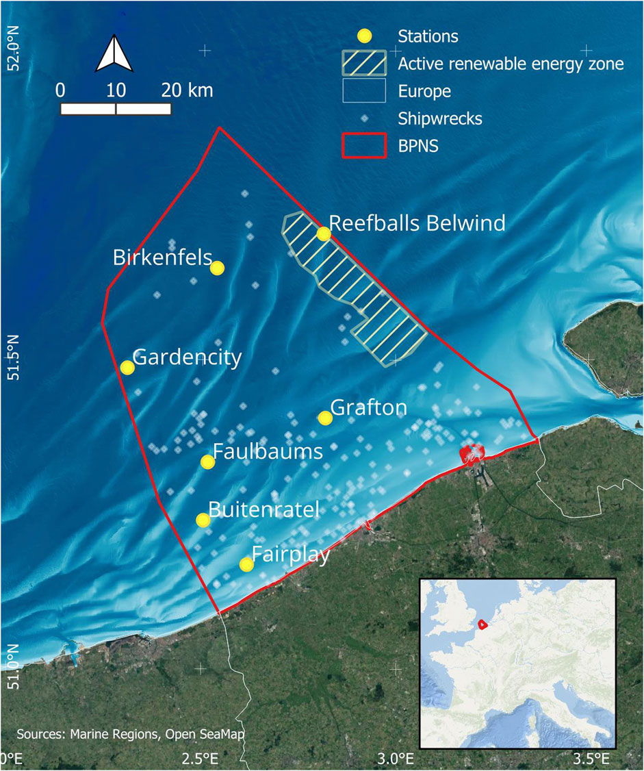
Figure 1. The stations of the LifeWatch Broadband Acoustic Network (Parcerisas et al., 2021) in the Belgian part of the North Sea (BPNS). Also shown in the map are the active renewable energy zone and shipwrecks.
Raw audio files used for annotation were manually chosen based on recording quality and possible presence of acoustically salient elements within the files, depending on environmental conditions such as period of the year, moment of the day, location and previously identified sound events. These annotations were part of an initial data exploration, and they were not annotated following a defined strategy. Only segments deemed to contain acoustically salient elements were annotated, with durations ranging from several minutes to several hours. Annotated samples were from four of the seven present stations, namely, Belwind, Birkenfels, Buitenratel and Grafton (Figure 1). The total duration of annotated samples per station is listed in Supplementary Table S1. All files were annotated using Raven Pro version 1.6.52, and the settings used during annotation are listed in Supplementary Table S2.
Audio events considered to be target events (acoustically salient) were meticulously identified and labeled by drawing boxes around each identified signal. All sounds were labeled, both known and unknown. This means that in addition to sounds possibly originating from marine organisms, other sounds labeled included anthropogenic and geophonic sounds.
Label tag names were cross-checked with tags available in underwater sound repositories, such as FishSounds (fishsounds.net) and Dosits (dosits.org). Sounds with similar acoustic characteristics to the descriptions found online were named accordingly. If a sound of interest could not be related to a sound from one of these online platforms, another tag name was chosen based on auditory characteristics exhibited by each sound. Sounds with similar shapes within the spectrogram, auditory characteristics, frequency range and duration were assigned the same tag name.
The absence of prior knowledge about the present biological sound sources posed a significant challenge, even when cross-checking with existing libraries. In response, rather than focusing on a time-intensive process of meticulously evaluating and classifying each sound type, an alternative approach was adopted where subjective categories were assigned to any encountered sound, irrespective of repetition or a pre-defined classification scheme, followed by clustering and revision of the identified sounds (see Section 2.4).
We decided to use automatic feature extraction and following statistical clustering of these features to group and describe unknown sounds. As it is not clear which are the best acoustic features to describe and differentiate unknown underwater sounds, we decided to use available published state-of-the-art deep learning algorithms pre-trained and/or tested in bioacoustics data, containing (at least, partly) underwater sounds. Two different options were considered, namely, the Animal Vocalization Encoder based on Self-Supervision (AVES; Hagiwara, 2023) and a convolutional autoencoder network (CAE; Best et al., 2023) to obtain acoustic features. Since the autoencoder approach is unsupervised, we trained it on our own data (for training details see Supplementary Table S3). AVES extracts the features directly from the waveform, which has the advantage that no parameters must be chosen manually to create a representative spectrogram. Conversely, CAE uses spectrograms as an input, and all the snippets need to be cut (or zero-padded) to a certain length before generating the spectrogram images. Both models were developed with the intention of being robust across datasets, by evaluating them on datasets which were not used to train the model. AVES was tested on data from birds, terrestrial mammals, marine mammals, insects (mosquitos) and amphibians (frogs), and CAE on data from different birds and marine mammals. Due to their proven generalizability, they were considered appropriate for this study.
Before the extraction of features, we filtered all manual annotations to have a minimum duration of 0.0625 s, a maximum duration of 10 s, a maximum low frequency of 24,000 Hz, and a minimum NIST-Quick SNR of 10 dB. For the annotations whose maximum high frequency exceeded 24,000 Hz the high frequency was adapted to 24,000 Hz. This assured that the characteristics of the remaining sounds complied with the requirements of the two feature extraction algorithms and assured the exclusion of false annotations. All sound files were decimated to 48,000 Hz before feature extraction to assure comparability in extracted features.
For each of the models, two different strategies were tested, leading to four different feature sets.
For the AVES-bio-base model, we first extracted snippets from the raw audio files using the start and end time of each annotation. These snippets were then band-pass filtered to the frequency limits of each annotation using a Butterworth filter of order four from the scipy Python package (Virtanen et al., 2020). The filtered snippet was then converted to audio representations using the AVES-bio model (1) subjected to mean-pooling (AVES-mean) or (2) subjected to max-pooling (AVES-max) to derive a 768-feature long vector per sound event for succeeding clustering analysis.
The CAE from Best et al. (2023) is applied to spectrogram representations of the sounds instead of raw waveforms. Therefore, Mel spectrograms were created from 3s-windows around the center time of an annotation with an NFFT value of 2048 and 128 Mel filterbanks and passed through the CAE with the bottleneck set to 256, deriving vectors of the same number (CAE-original). As a modification to this to better represent the large variabilities in duration and bandwidth that we observed among the annotated unknown sounds in our data, we also trained the CAE network with cropped spectrograms to their start and end times and low and high frequency limits (CAE-crops). For this, spectrograms were created for the actual duration of the sound event with an NFFT value chosen to deliver at least 128 frequency bins between the minimum and the maximum frequency, and the window overlap was set to deliver at least 128 time slots. The resulting spectrogram matrix was then cropped to the actual frequency limits of the sound event. To achieve compliance with the input format to the CAE, all resulting spectrogram images were then reshaped to 128 × 128 bins before they were also passed through the CAE with the bottleneck set to the default number of 256, based on the study of Best et al. (2023) on varying bottleneck sizes. This derived vectors of 256 features at the end. For both CAE approaches (CAE-original and CAE-crops), the audio snippets were filtered to the frequency limits of the annotations using the same filtering strategy as for AVES, a band-pass Butterworth filter of order four from the scipy Python package (Virtanen et al., 2020).
To all four different types of feature vectors, we added four additional features which were directly extracted from the Raven selection tables, namely, low frequency, high frequency, bandwidth and duration.
Feature selection is often conducted in large and high-dimensional datasets prior to applying clustering algorithms to get a subset of features which will best discriminate the resulting clusters (Dash and Liu, 2000). This was done because most clustering algorithms do not perform well in high dimensional space, a problem known as “the curse of dimensionality”. First, using the scikit-learn Python library (Pedregosa et al., 2011), the feature sets were centered to the mean and scaled to unit variance. Then, sparse Principal Component Analysis (sPCA) was applied to reduce the four feature sets to the most discriminant features. sPCA forms principal components with sparse loadings—each principal component (PC) resulting to a subset of principal variables, in contrast to ordinary Principal Component Analysis (PCA) wherein each PC is a linear combination of all original variables (Zou et al., 2006). The four additional features—low frequency, high frequency, bandwidth and duration, were retained in addition to the sPCA-selected features.
Upon choosing a clustering algorithm that would give meaningful clusters from our annotations, two aspects of the dataset were of concern due to the manner of annotation done in this study: (1) the variation among cluster densities as the selection of recording files to annotate was not done in a standardized manner, and (2) the presence of noise, or falsely annotated samples in the datasets, due to the inherent nature of annotations on underwater sounds, especially when the source is unknown. Therefore, an unsupervised density-based clustering algorithm, HDBSCAN (McInnes et al., 2017), based on hierarchical density estimates was chosen. HDBSCAN partitions the samples according to the most significant clusters with varying density thresholds, excluding samples that are identified as noise by the algorithm itself (Campello et al., 2013). The clustering was applied to the sPCA-reduced CAE (CAE-original and CAE crops) and AVES (AVES-mean and AVES max) feature sets (Figure 2).
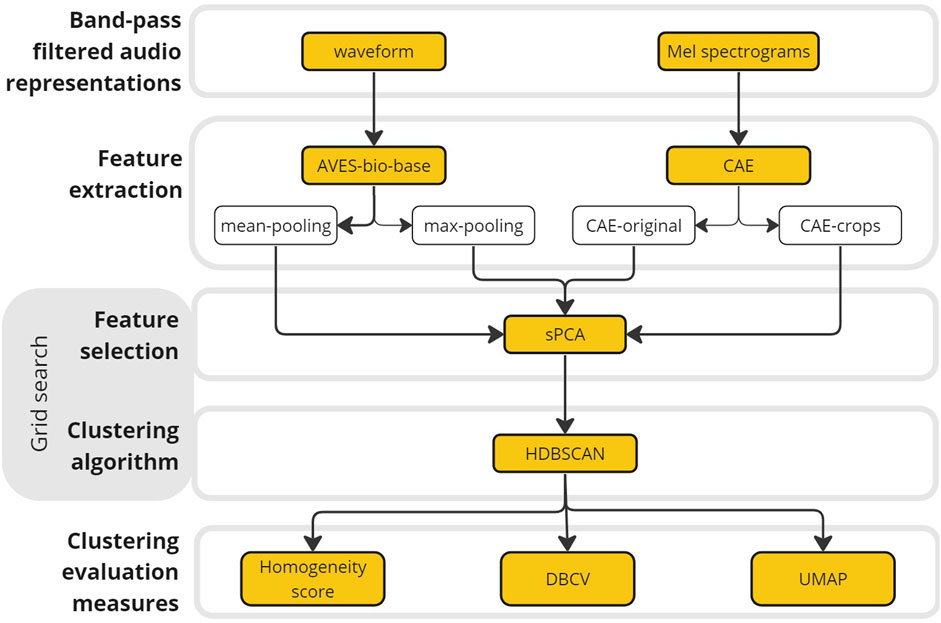
Figure 2. Overview of the methodology conducted in this study from two different audio representations up to cluster evaluation measures. After feature extraction using the Animal Vocalization Encoder based on Self-Supervision (AVES) and a convolutional autoencoder network (CAE), the dimensionality of the datasets was reduced by selecting relevant features using sparse Principal Component Analysis (sPCA). Different values of the hyperparameters of sPCA and HDBSCAN were tested using a coded grid search function. Obtained clusters were evaluated using its homogeneity score and density-based clustering validation (DBCV) score, and visualized using Uniform Manifold Approximation and Projection (UMAP).
We coded a grid search function to adjust the hyperparameters of sPCA and HDBSCAN. We searched the hyperparameter space for the most optimized combination of parameter values based on two selected clustering evaluation measures: (1) the homogeneity score score from the scikit-learn Python library (Pedregosa et al., 2011) based on annotations, and (2) the density-based clustering validation (DBCV) score from the DBCV library (Jenness, 2017), based on the quality of clusters and not the annotations. Both scores range from 0 to 1, with one representing a perfect score. The homogeneity score compares the similarity of original annotations with the predicted clusters, wherein a score of one satisfies homogeneity of all predicted clusters (Rosenberg and Hirschberg, 2007). The DBCV score is an index proposed for density-based clusters which are not necessarily spherical. This score is based on the density of samples in a cluster, and the within- and between-cluster distances (Moulavi et al., 2014).
We inspected which parameters had a drastic effect on the resulting clusters and must be adjusted, prior to conducting grid search. For sPCA, only the parameter alpha, which controls the sparseness of components, was adjusted. The higher the alpha, the sparser the components, resulting to a lower number of ‘relevant’ features. We set different values of alpha (Supplementary Table S4, Supplementary) according to the range of features that formed reasonable/acceptable clusters during the data exploration phase of the study. For HDBSCAN, a grid of values based on three parameters–the minimum cluster size (5, 8, 10 and 12), the minimum samples (3, 4 and 5), and epsilon (0.2, 0.5, 0.8)–were specified. While the minimum cluster size specifies the smallest number of samples to form a cluster, the minimum samples parameter is the number of neighboring points to be considered a dense region, therefore restricting the formation of clusters to the denser areas and classifying more samples as noise. The epsilon value is a threshold by which a cluster is split into smaller denser clusters (McInnes et al., 2016).
For selecting the best clustering result from the grid search function, criteria had to be defined as high scores do not directly translate to high clustering performances. Performance is also based on the number of samples classified as noise and the number of resulting clusters. The following criteria were therefore set: (1) the percentage of samples clustered is >15%; that is, only a maximum of 85% of samples classified as noise by HDBSCAN was acceptable, (2) the number of clusters is ≤ the original number of annotation classes, and (3) with the highest average of homogeneity and DBCV scores. For visual comparative analysis, each grid search clustering result was also embedded into Euclidean space using a uniform manifold approximation and projection (UMAP; McInnes et al., 2020) with a number of neighbors equal to 15 and a minimum distance of 0.2. Significant differences in the homogeneity and DBCV scores among the four feature sets were tested using the non-parametric Kruskal–Wallis test (Kruskal and Wallis, 1952). Pairwise comparisons were performed using a Wilcoxon rank sum test (Wilcoxon, 1945) as a post-hoc. To test the association of the parameters with the two scoring metrics, the parameters were fitted in a generalized linear model (GLM) with a Gamma distribution using the ‘stats’ R package. Finally, predicted clusters from the best grid search result were then revised by a bioacoustics expert (J.A.) and one representative sound was chosen per cluster, which had a good SNR and the highest resemblance to the other sounds within the same cluster. Intra- and inter-cluster variation were assessed using the ‘clv’ R package (Nieweglowski, 2023) and visualized using the ‘qgraph’ R package (Epskamp et al., 2023). Intra-cluster distance was calculated as the distance between the two furthest points within each cluster, while inter-cluster distances was calculated for each possible pair of cluster as the average distance between all samples of two different clusters.
An overview of the methodology from feature extraction up to evaluation of clusters is shown in Figure 2. Feature extraction and unsupervised clustering were performed using Python version 3.11.5 (Python developers, 2023), while statistical tests were performed using R version 4.3.1 (R Core Team, 2023), with scripts made available on the GitHub repository: https://github.com/lifewatch/unknown_underwater_sounds.
From all the selected raw audio files from the LifeWatch Broadband Acoustic Network in the BPNS, there were 2,874 target sounds of interest, annotated with 30 different tags (Figure 3). From all the annotations, those whose source could be identified and were not of biological origin were excluded from the analysis. These included boat noises, out of water sounds, water movements, deployment sounds, electronic noises and interferences. Acoustic features extracted through AVES and CAE were each reduced through sPCA. Different values of alpha were embedded in the grid search giving a similar range (15–31) of principal features for each dataset (Supplementary Table S4). The different values of sPCA alpha in combination with the different HDBSCAN clustering parameters (epsilon, minimum cluster size and minimum samples) gave a total of 431 grid search results.
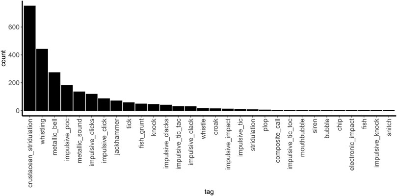
Figure 3. Annotated samples with corresponding tags in the Belgian part of the North Sea (BPNS), which excluded audio events related to boat operations, water movements, deployment operations, electronic noises and interference.
Of the total 431 grid search results, only 238 results met the criteria set in this study with percentage of samples clustered >15% (>431 annotated samples) and the number of clusters less than or equal to the number of original annotation tags (=30). From these 238 grid search results, where the same parameters regardless of the epsilon value gave the same homogeneity and DBCV scores, we only kept the grid search result with the highest epsilon value—further narrowing down the 238 grid search results to 149. Within these 149 grid search results, homogeneity scores ranged from 0.005 to 0.800, DBCV scores from 0.221 to 0.837 and the average of the two scores from 0.240 to 0.687 (Figure 4). Seven (CAE-crops and CAE-original) and four (CAE-crops) grid search results had homogeneity and DBCV scores considered outliers, respectively. The means and standard deviations of the scores from the grid search for each feature set are detailed in Supplementary Table S5.
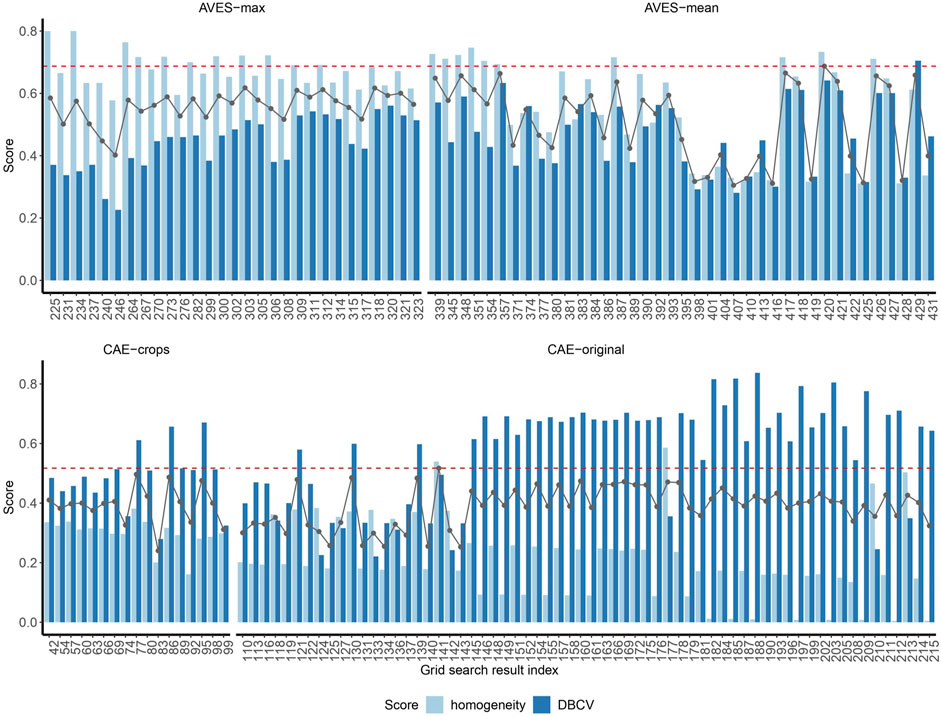
Figure 4. Homogeneity and density-based clustering validation (DBCV) scores of the 149 grid search results (indicated by the grid search result indices on the x-axis) grouped by feature set. The black dotted lines indicate the average of the two scores, while the red dashed line indicates the highest average score among the grid search results within AVES and CAE feature sets.
Homogeneity and DBCV scores were significantly different among the feature sets (Figure 5; Kruskal–Wallis test, p = 2.2–16 [homogeneity], p = 0.0001 [DBCV]). Pairwise comparisons using Wilcoxon rank sum test showed that homogeneity scores among the four feature sets were significantly different from each other (p < 0.05). Likewise, the same test showed that DBCV scores were significantly different between the AVES feature sets and CAE-original (all p < 0.05). While AVES-max and AVES-mean feature sets had higher homogeneity scores, DBCV scores were higher for CAE-original. Finally, fitting all parameters in a GLM (details in Supplementary Table S6; Supplementary Figure S1), the number of features was significantly associated to DBCV (p = 5.960–5), and the minimum cluster size to homogeneity scores (p = 9.864–5).
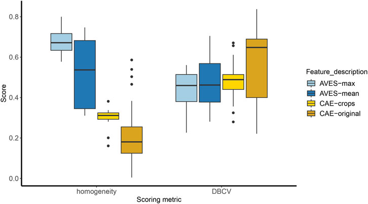
Figure 5. Boxplots of homogeneity and density-based clustering validation (DBCV) scores for the four feature sets (AVES-max, AVES-mean, CAE-crops and CAE-original). Homogeneity scores were significantly different between each feature set (all p < 0.05). DBCV scores were significantly different between the AVES feature sets and CAE-original (p = 0.001).
Among the AVES feature sets, grid search result index # 420 (AVES-mean) had the highest average of homogeneity and DBCV scores (=0.687), with the number of features reduced to 15. There were 635 samples (22% of the total samples) that were clustered with a minimum cluster size of 10. Among the CAE feature sets, grid search result index # 141 (CAE-original) ranked with the highest average score (=0.517), with features reduced to 31. There were 1,279 samples (45% of the total samples) that were clustered, with a minimum cluster size of 12. The UMAP embeddings of grid search results # 420 and # 141 (best of each approach) show a considerable separation between most of the clusters (Figure 6), with bigger clusters more evident from the UMAP embedding of grid search result index # 141 (Figure 6B).
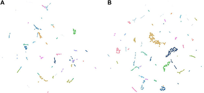
Figure 6. Uniform Manifold Approximation and Projection (UMAP) of the 26 predicted clusters from grid search result # 420 (AVES-mean; (A) and the 29 predicted clusters from grid search result # 141 (CAE-original; (B), which had the highest average of homogeneity and DBCV scores among the AVES and CAE feature sets, respectively.
The best grid search result index # 420, with a homogeneity score of 0.733 and DBCV score of 0.641, yielded 26 clusters (Figure 7). Descriptions of the resulting sound categories are summarized in Table 1. Spectrograms of representative sound tags are shown in Figure 8 and Supplementary Figure S2. Of the 26 clusters, seven were completely homogeneous (clusters 3, 4, 7, 21, 22, 23 and 24; Figure 7)—that is, samples within each of those clusters were labeled with the same tags during annotation. Two additional clusters (15 and 16) were assessed as completely homogeneous after revision. Of the total nine completely homogeneous clusters, six were represented by ‘Whistling’, two of ‘Tick’ and one of ‘Metallic Bell’. Two clusters (10 & 20) had less than 50% homogeneity: cluster 10 was composed of tags ‘Crustacean Stridulation’, ‘Impulsive Clack’, ‘Jackhammer’ and ‘Fish Grunt’, while cluster 20 was composed of ‘Impulsive Poc’, ‘Crustacean Stridulation’, ‘Fish Grunt’, ‘Knock’ and ‘Plop’. Multiple clusters represented by the same sound, such as clusters represented by ‘Whistling’, ‘Impulsive Poc’, ‘Impulsive Click’ and ‘Tick’, had lower inter-cluster distances, but also relatively high intra-cluster distances (Figure 10). Additionally, a clear separation between subgroups of clusters under ‘Whistling’ and ‘Crustacean Stridulation’ can be observed. Separation of clusters 3–4 and 21–24, all represented by ‘Whistling’, and clusters 1, 10, 5 and 6, all represented by ‘Crustacean Stridulation’, indicates variation in acoustic representations within the same classification of sound.
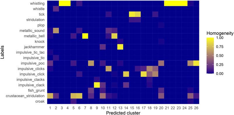
Figure 7. Agreement of annotations with predicted clusters of grid search result # 420. The grids are shaded by the percentage of occurrence of a tag within a predicted cluster.
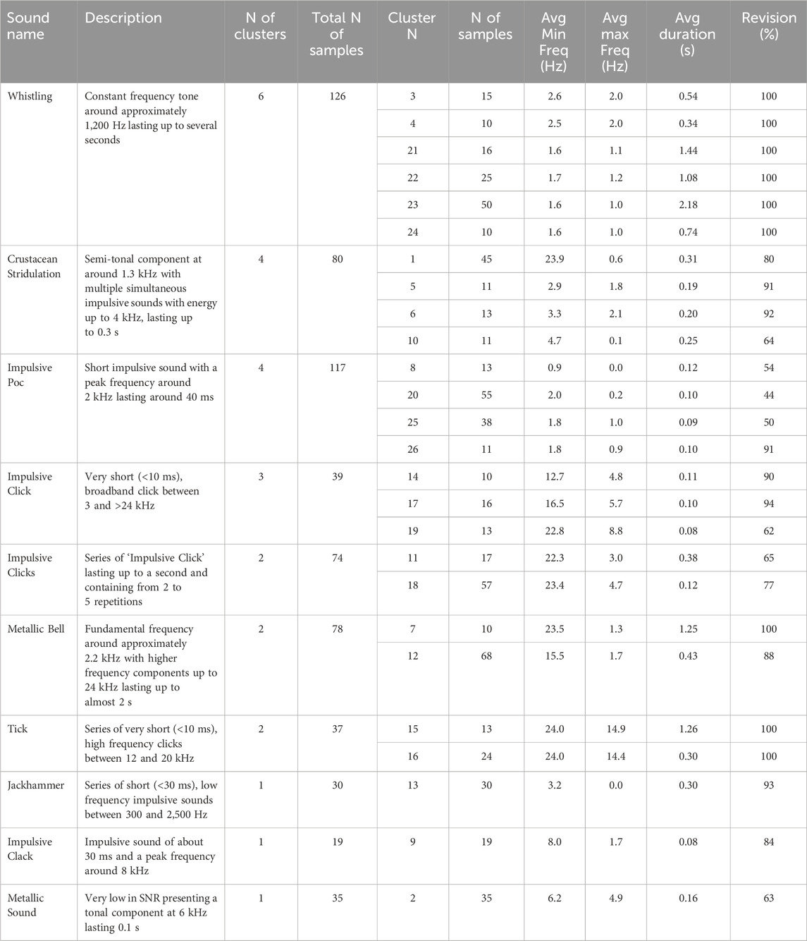
Table 1. Summary of descriptions of the obtained sound types after clustering. Spectrogram representations of each cluster are plotted in Supplementary Figure S2. N refers to “number” and Avg to “average”. Revision (%) shows the number of samples correctly clustered.
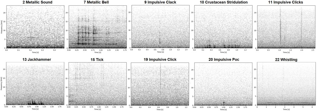
Figure 8. Spectrograms of revised clusters from the best grid search result which had the highest average of homogeneity and DBCV scores. Each spectrogram is labeled by the cluster # and the representative sound tag which had the highest resemblance to the other sounds from the same cluster.
The lack of reliable annotated training datasets and sound libraries is a critical methodological gap in studying soundscapes where sound sources are unknown. Our study demonstrated that unsupervised clustering of annotated unknown sounds eases revision and validation of annotated datasets. The revised clusters (Figure 8) we detailed already define a few groups of recurring distinct sounds that could serve as a preliminary component of an annotated training dataset. Annotation and labeling, in the absence of a reference dataset with validated annotations, are arduous and subjective especially for an underwater soundscape such as the BPNS, where sound signatures are unknown and the inherent acoustic scene is complex (Parcerisas et al., 2023b). Although unsupervised clustering is conventional in ecological research (Sainburg et al., 2020; Schneider et al., 2022; Guerrero et al., 2023), we highlight its practical use in revising clusters of annotated unknown sounds. Unsupervised clustering and subsequent revision of obtained clusters are therefore proposed steps to systematically reduce annotations to distinct and recurring sound events deemed relevant (Figure 9). With the proposed approach, labeling efforts only become a requisite for unclassified sounds of interest from newly gathered data, which do not fall under the same classification as the obtained revised clusters when clustered together with the old data, potentially forming new clusters. Sounds falling under the obtained clusters would not need to be manually labeled then. This approach speeds up the entire process of future human annotations and labeling efforts. The obtained datasets can be used for supervised ML (Figure 9), provided that the built training dataset is sufficient. Supervised ML models would render automatic detections and classification of already named and characterized sound signatures, whether the source is known or unknown. Human labeling and classifying efforts of these distinct and recurring sound events would then become unnecessary in the future.
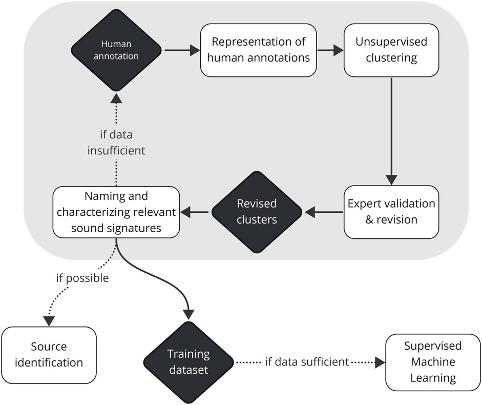
Figure 9. Proposed steps to build a validated training dataset that can feed supervised machine learning (ML) models for unknown soundscapes. Unsupervised clustering is applied to representations of human annotations. Robust clusters, revised and validated by an expert, are named and characterized, and when possible, their sources are identified. The steps from human annotation to naming and characterization of relevant sound signatures (enclosed in a grey rectangle) are repeated in a cycle until the training dataset is sufficient to feed supervised ML models.
The most crucial step to achieve a meaningful characterization of recurring unknown sound signatures with our approach is the formation of relevant clusters. Two factors largely influenced the formation of clusters: (1) obtaining a relevant feature representation of the annotated dataset and (2) adjusting the hyperparameters of the chosen algorithms. Slight changes in any configuration altered the quality of clusters obtained. For instance, the choice of subjecting AVES feature sets to mean- or max-pooling (AVES-mean vs. AVES-max) or cropping spectrogram representations to the actual frequency limits and duration of the sound event (CAE-crops vs. CAE-original), accounted for significant differences in the homogeneity and shape of formed clusters (Figure 5). Selecting different minimum sizes of clusters significantly affected homogeneity scores, and the number of relevant features significantly affected DBCV scores.
While selecting the best representation model to extract features and applying the most appropriate clustering method have been obvious factors to consider in bioacoustics research, we highlight the performance variations brought by the large search space of hyperparameter configurations (Best et al., 2023) which have remained obscure in the literature. As these configurations, mostly related to hyperparameters of algorithms, are often ambiguous and dataset-specific, grid search is therefore a step that should be considered when applying any algorithm. Though deep learning features, such as AVES and CAE, can be used efficiently by neural networks to classify sounds, not all extracted features are directly representative for any dataset. Varying numbers of selected discriminant features in the grid search using sparse PCA contributed to performance variation. Although, due to time-constraint, we only revised the best clustering result with the highest average of homogeneity and DBCV scores, it is also possible to revise other clustering results which performed as well, such as grid search result index # 141 (CAE-original).
In evaluating clustering performance, understanding the reliability of annotations determines the type of scoring metrics. As manual annotations made by a single individual are not fully reliable, additionally scoring the clusters through an unsupervised metric (DBCV) allowed for a reasonable evaluation of cluster quality. Scoring metrics must be cautiously interpreted, however, as high scores do not necessarily translate to relevant clusters. We excluded 43% of our grid search results from subsequent analyses, although some of these had higher homogeneity or DBCV scores, since these either gave too many clusters of the smallest size possible or very few clusters of the largest size possible, with more than 85% of the samples rejected by HDBSCAN. With highly conservative clusters, higher homogeneity and DBCV scores are obviously easier to achieve but would defeat the purpose of grouping vocalization repertoires per species or sounds derived from the same source in the same cluster. As a consequence of underwater sound variability (both in sound production and reception), sounds could possibly be originating from the same source yet either grouped into several smaller clusters, or classified as noise by HDBSCAN, due to slight differences in selected acoustic representation. The similarity of multiple clusters within the same classification of sound was evident in clusters represented by ‘Whistling’, ‘Impulsive Poc’, ‘Impulsive Click’ and ‘Tick’ (Figure 10). However, in some cases, variation within a cluster could be just as large as the variation between clusters represented by different sounds such as ‘Crustacean Stridulation’ (clusters 1, 10, 5, 6) and ‘Whistling’ (clusters 3–4 and clusters 21–24). This highlights the difficulty of manually categorizing and naming unidentified sound types. Multiple clusters of the same sound could arise from signals of varying SNRs, including the environmental noise of a recording station (Baker and Logue, 2003), overlapping in time and frequency (Izadi et al., 2020). Reception of signals can also differ due to differences in sound propagation and frequency-dependent loss brought by largely varying distances from the source (Forrest, 1994). This is common in harmonic sounds such as the ‘Metallic Bell’ where some clusters have less harmonics visible in the spectrogram. However, multiple clusters of the same sound could also be partly due to our imbalanced annotations, which is highly dominated by ‘Crustacean Stridulation’, ‘Whistling’, ‘Impulsive Poc’, ‘Metallic Bell’, ‘Impulsive Click’, ‘Impulsive Clicks’ and ‘Tick’ (Figure 3). Thus, small numbers of minimum cluster size and minimum samples were necessary to consider tags in the annotations with only a few samples. Since vocal repertoires remain unknown in the BPNS to date, we rely on this growing dataset to detect apparent and consistently similar sounds which are likely of the same origin. In the future, with a bigger dataset composed of annotations that are more representative of the BPNS soundscape, an ample number of bigger and denser clusters is plausibly easier to obtain.
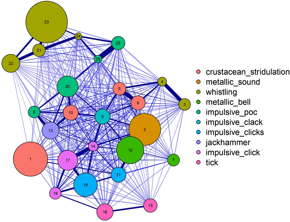
Figure 10. Evaluation of intra- and inter-cluster distances between each cluster. Clusters are separated by inter-cluster distance. Line thickness indicates similarity between each cluster. Clusters are numbered according to the cluster number and colored by the representative sound.
Presently, there is no standard in annotating datasets, or which acoustic features should be used in bioacoustics research, when deciding whether two sounds are from the same source (Odom et al., 2021; Schneider et al., 2022). In the present work, AVES and CAE performed differently depending on model configurations and hyperparameters. Meaningful clusters were obtainable from both models, although AVES-mean consistently ranked with the best scores since the exploration phase of this study. AVES feature sets resulted in more solid, homogeneous clusters with relatively lower intra-cluster distances, appearing to be more advantageous for the purpose of obtaining distinct clusters of recurring sounds with precision in this dataset. However, AVES clusters were disadvantaged by the relatively higher percentage of samples classified as noise by HDBSCAN. With CAE feature sets, a higher number of samples (68% on average) were clustered, but this resulted in more scattered and less homogeneous clusters which entail greater effort in manual revision. This could be due to the diversity of sound duration and frequency bands, hence no spectrogram parameters were found which could visually represent all different sound types appropriately. Furthermore, CAE was re-trained on our annotations containing only 2,875 examples, which might not be enough for a deep learning model. CAE might be more effective in representing datasets with a more uniform distribution in both sound duration and frequency boundaries, because then it is possible to ensure that all the spectrograms fed to the model are meaningful for all the annotations using the same parameters. CAE might also be more effective when trained on bigger datasets, such as those from biologically rich environments with a large amount of similar fish sounds. A possible approach to deal with the data limitation would be to use data augmentation techniques when training the model (Nanni et al., 2020). This could include, for example, training on both the original and the cropped spectrograms. The rigor of these models and the influence of hyperparameters must be continuously explored.
Though the purpose of this study was to obtain clusters of recurring sounds, a density-based clustering algorithm such as the HDBSCAN could potentially omit extremely infrequent sound types with insufficient data by classifying these as noise. Extremely rare sounds, which occurred less than five times in the dataset (e.g., snitch, impulsive knock, fish, electronic impact, bubble, siren, mouthbubble, impulsive tic toc and composite call; Figure 3), were classified as noise by the clustering algorithm as we expected. Separating rare sounds, which were not encountered on multiple occasions, from actual noise is a common clustering limitation that consequently underrepresents what is essentially a more biologically diverse soundscape. Denoising and processing signals prior to clustering can improve unsupervised learning, such as source separation techniques (Sun et al., 2022; Lin and Kawagucci, 2024). However, there is currently no algorithm that satisfactorily addresses a broad spectrum of conditions for bioacoustics data in general, and marine bioacoustics in particular (Xie et al., 2021; Juodakis and Marsland, 2022). For this reason, during a preliminary exploration of the feature extraction algorithms, we compared the results obtained when (1) applying a non-stationary noise reduction algorithm (Sainburg et al., 2024), (2) no filter is applied, and (3) applying a band-pass filtering to each snippet. The results showed that for this dataset with such a variety of sounds, the band-pass filtering yielded the best results which could be due to several reasons. Firstly, for AVES and CAE-original, it allows for distinguishing between sounds occurring simultaneously at different frequency bands, which otherwise would be confused by the models. This is not the case for non-stationary noise reduction strategies, as both events happening simultaneously would be enhanced. Secondly, for low SNR annotations, a clearer signal can be obtained. Noise reduction algorithms such as noisereduce can enhance the SNR of signals, but they can perform badly for such short sounds such as ‘Impulsive Click’.
While the complex acoustic scene of the BPNS has been previously described (Parcerisas et al., 2023b), sound signatures, especially of biological sources, remain unclear and unidentified. Of the final revised clusters in the present work, we were able to name and describe 10 unique sounds (Figures 8, 10). However, only cluster 13 with the ‘Jackhammer’ sounds and clusters 15 and 16 with the ‘Tick’ sounds can be interpreted as biological with some certainty. The ‘Jackhammer’ sounds fit within the known vocalization frequency range of fish (<3 kHz) and is a repetitive set of impulse sounds (Amorim, 2006; Carriço et al., 2019). They resemble sounds produced by fish species from the family Sciaenidae (Amorim et al., 2023) and occurrences of an invasive species of this family have been also documented for the North Sea (Morais et al., 2017). The short duration, high frequency ‘Tick’ sounds are similar to crustacean acoustic signals, which are known to span a large range of frequencies (Edmonds et al., 2016; Solé et al., 2023). While ‘Metallic Bell’ is largely supposed as mooring noise, we do not fully dismiss the possibility that it is biological. It has high resemblance to recorded sounds (although from a glass tank) of a spider crab Maja brachydactyla (Coquereau et al., 2016), which is present in the BPNS and often found in our moorings. However, these are just speculations as no ground-truth has been confirmed and further research would be necessary to assign the species to the sound with certainty. All other clustered sounds can only be interpreted with caution (e.g., ‘Metallic Sound’ could be a chirp of a mammal, ‘Whistling’ could be an anthropogenic sound originating from boats or geophony caused by wind, and ‘Crustacean Stridulation’ could be something called bio-abrasion, namely, the mechanical disturbance of the recorder by an animal–Ryan et al., 2021) as, to our knowledge, there are no similar sounds described in the literature so far. Spatiotemporal analyses of sound occurrence (which was not achievable in this study due to biases during data selection), alongside detailed comparisons of the acoustic characteristics of encountered sounds, are therefore necessary to further infer the possible biological sources of identified sounds.
Apart from AVES and CAE, there are numerous feature extraction models in the literature which perform differently from case-to-case. For example, Ozanich et al. (2021) adds an extra clustering layer to an autoencoder similar to the CAE model to penalize points that are distant from cluster centers. If licenses of required MATLAB toolboxes are present, the software CASE (Cluster and Analyze Sound Events; Schneider et al., 2022) can be freely downloaded for the purpose of selecting an appropriate clustering algorithm among four methods (community detection, affinity propagation, HDBSCAN and fuzzy clustering) and three classifiers (k-nearest neighbor, dynamic time-warping and cross-correlation) iterated over different values of parameters. Results are then subsequently evaluated using normalized mutual information (NMI), a scoring metric similar to the homogeneity score which relies on the level of agreement with pre-labeled data. If pre-labeled data are absent or highly unreliable due to the unidentified nature of the labels, we recommend coding a grid search function to easily compare results of differently tuned algorithms. Since incorporating gained information by different research groups is often difficult, we echo the pressing need for GLUBS (Parsons et al., 2022) which will highly benefit bioacoustics research of unknown soundscapes such as the BPNS.
The dataset presented in this study can be found in online repositories such as the Marine Data Archive (MDA) and Integrated Marine Information System (IMIS; https://doi.org/10.14284/659).
AC: Formal Analysis, Investigation, Methodology, Software, Visualization, Writing–original draft, Writing–review and editing. CP: Conceptualization, Data curation, Investigation, Methodology, Software, Writing–review and editing. ES: Investigation, Methodology, Software, Validation, Visualization, Writing–original draft, Writing–review and editing. ED: Funding acquisition, Project administration, Resources, Supervision, Writing–review and editing.
The author(s) declare that financial support was received for the research, authorship, and/or publication of this article. This research was funded by LifeWatch grant number I002021N. ES’s contribution to this research was funded by FWO grant number V509723N.
This work demonstrated LifeWatch observation data, which made use of infrastructure (the broadband acoustic network) provided by VLIZ and funded by Research Foundation - Flanders (FWO) as part of the Belgian contribution to LifeWatch. A lot of hands contributed to the maintenance of the network—we thank the Marine Observation Center and Infrastructure department of VLIZ and the crew of RV Simon Stevin for their continuous involvement and support at sea. Last but not least, we thank Coline Bedoret for her dedication in annotating the recordings over the summer of 2023, and Julia Aubach for revising the clusters.
The authors declare that the research was conducted in the absence of any commercial or financial relationships that could be construed as a potential conflict of interest.
All claims expressed in this article are solely those of the authors and do not necessarily represent those of their affiliated organizations, or those of the publisher, the editors and the reviewers. Any product that may be evaluated in this article, or claim that may be made by its manufacturer, is not guaranteed or endorsed by the publisher.
The Supplementary Material for this article can be found online at: https://www.frontiersin.org/articles/10.3389/frsen.2024.1384562/full#supplementary-material
Amorim, M. C. P. (2006). “Diversity of sound production in fish,” in Communication in fishes. Editors F. Ladich, S. Collin, P. Moller, and E. Kapoor (Enfield: Science Publishers), 71–105.
Amorim, M. C. P., Wanjala, J. A., Vieira, M., Bolgan, M., Connaughton, M. A., Pereira, B. P., et al. (2023). Detection of invasive fish species with passive acoustics: discriminating between native and non-indigenous sciaenids. Mar. Environ. Res. 188, 106017. doi:10.1016/j.marenvres.2023.106017
Baker, M. C., and Logue, D. M. (2003). Population differentiation in a complex bird sound: a comparison of three bioacoustical analysis procedures. Ethology 109, 223–242. doi:10.1046/j.1439-0310.2003.00866.x
Best, P., Paris, S., Glotin, H., and Marxer, R. (2023). Deep audio embeddings for vocalisation clustering. PLOS ONE 18, e0283396. doi:10.1371/journal.pone.0283396
Campello, R. J. G. B., Moulavi, D., and Sander, J. (2013). “Density-based clustering based on hierarchical density estimates,” in Pacific-asia conference on knowledge discovery and data mining. Editors J. Pei, V. S. Tseng, L. Cao, H. Motoda, and G. Xu (Gold Coast, Australia: Springer Berlin Heidelberg), 160–172. doi:10.1007/978-3-642-37456-2_14
Carriço, R., Silva, M. A., Meneses, G. M., Fonseca, P. J., and Amorim, M. C. P. (2019). Characterization of the acoustic community of vocal fishes in the Azores. PeerJ 7, e7772. doi:10.7717/peerj.7772
Cato, D., McCauley, R., Rogers, T., and Noad, M. (2006). “Passive acoustics for monitoring marine animals - progress and challenges,” in New Zealand, (christchurch, New Zealand: Australian and New Zealand acoustical societies), 453–460.
Coquereau, L., Grall, J., Chauvaud, L., Gervaise, C., Clavier, J., Jolivet, A., et al. (2016). Sound production and associated behaviours of benthic invertebrates from a coastal habitat in the north-east Atlantic. Mar. Biol. 163, 127. doi:10.1007/s00227-016-2902-2
Cotter, A. J. R. (2008). “The ‘soundscape’ of the sea, underwater navigation, and why we should be listening more,” in Advances in fisheries science. Editors A. Payne, J. Cotter, and T. Potter (New Jersey, United States: Wiley), 451–471. doi:10.1002/9781444302653.ch19
Dash, M., and Liu, H. (2000). “Feature selection for clustering,” in Lecture notes in computer science. Editors T. Terano, H. Liu, and A. L. P. Chen (Berlin Heidelberg: Springer). doi:10.1007/3-540-45571-X_13
Degraer, S., Brabant, R., Rumes, B., and Virgin, L. (2022). Environmental impacts of offshore wind farms in the Belgian part of the North Sea: getting ready for offshore wind farm expansion in the North Sea. Brussels: royal Belgian Institute of natural sciences, operational directorate natural environment. Mar. Ecol. Manag.
Duarte, C. M., Chapuis, L., Collin, S. P., Costa, D. P., Devassy, R. P., Eguiluz, V. M., et al. (2021). The soundscape of the Anthropocene ocean. Science 371, eaba4658. doi:10.1126/science.aba4658
Edmonds, N. J., Firmin, C. J., Goldsmith, D., Faulkner, R. C., and Wood, D. T. (2016). A review of crustacean sensitivity to high amplitude underwater noise: data needs for effective risk assessment in relation to UK commercial species. Mar. Pollut. Bull. 108, 5–11. doi:10.1016/j.marpolbul.2016.05.006
Epskamp, S., Constantini, G., Haslbeck, J., Isvoranu, A., Cramer, A., Waldorp, L., et al. (2023). Package “qgraph”. Available at: https://cran.r-project.org/web/packages/qgraph/qgraph.pdf.
Forrest, T. G. (1994). From sender to receiver: propagation and environmental effects on acoustic signals. Am. Zool. 34, 644–654. doi:10.1093/icb/34.6.644
Gage, S. H., and Farina, A. (2017). “Ecoacoustics challenges,” in Ecoacoustics. Editors A. Farina, and S. H. Gage (New Jersey, United States: Wiley), 313–319. doi:10.1002/9781119230724.ch18
Guerrero, M. J., Bedoya, C. L., López, J. D., Daza, J. M., and Isaza, C. (2023). Acoustic animal identification using unsupervised learning. Methods Ecol. Evol. 14, 1500–1514. doi:10.1111/2041-210X.14103
Hagiwara, M. (2023). “AVES: animal vocalization encoder based on self-supervision,” in ICASSP 2023 - 2023 IEEE International Conference on Acoustics, Speech and Signal Processing (ICASSP), (Rhodes Island, Greece: IEEE), Rhodes Island, Greece, 4-10 June 2023, 1–5.
Houziaux, J.-S., Haelters, J., and Kerckhof, F. (2007) Biodiversity science: a case study from Belgian marine waters. Copenhagen: International council for the exploration of the sea. Available at: https://www.vliz.be/imisdocs/publications/135511.pdf.
Izadi, M. R., Stevenson, R., and Kloepper, L. N. (2020). Separation of overlapping sources in bioacoustic mixtures. J. Acoust. Soc. Am. 147, 1688–1696. doi:10.1121/10.0000932
Jenness, C. (2017). DBCV. Available at: https://github.com/christopherjenness/DBCV.
Juodakis, J., and Marsland, S. (2022). Wind-robust sound event detection and denoising for bioacoustics. Methods Ecol. Evol. 13, 2005–2017. doi:10.1111/2041-210X.13928
Kerckhof, F., Rumes, B., and Degraer, S. (2018). A closer look at the fish fauna of artificial hard substrata of offshore renewables in Belgian waters. Available at: https://core.ac.uk/download/pdf/168393142.pdf.
Kruskal, W. H., and Wallis, W. A. (1952). Use of ranks in one-criterion variance analysis. J. Am. Stat. Assoc. 47, 583–621. doi:10.1080/01621459.1952.10483441
Leroy, E. C., Thomisch, K., Royer, J.-Y., Boebel, O., and Van Opzeeland, I. (2018). On the reliability of acoustic annotations and automatic detections of Antarctic blue whale calls under different acoustic conditions. J. Acoust. Soc. Am. 144, 740–754. doi:10.1121/1.5049803
Lin, T., and Kawagucci, S. (2024). Acoustic twilight: a year-long seafloor monitoring unveils phenological patterns in the abyssal soundscape. Limnol. Oceanogr. Lett. 9, 23–32. doi:10.1002/lol2.10358
Lindseth, A., and Lobel, P. (2018). Underwater soundscape monitoring and fish bioacoustics: a review. Fishes 3, 36. doi:10.3390/fishes3030036
Looby, A., Erbe, C., Bravo, S., Cox, K., Davies, H. L., Di Iorio, L., et al. (2023). Global inventory of species categorized by known underwater sonifery. Sci. Data 10, 892. doi:10.1038/s41597-023-02745-4
McInnes, L., Healy, J., and Astels, S. (2016). The hdbscan clustering library parameter sel HDBSCAN. Available at: https://hdbscan.readthedocs.io/en/latest/index.html.
McInnes, L., Healy, J., and Astels, S. (2017). hdbscan: hierarchical density based clustering. J. Open Source Softw. 2, 205. doi:10.21105/joss.00205
McInnes, L., Healy, J., and Melville, J. (2020). UMAP: uniform manifold approximation and projection for dimension reduction. Available at: http://arxiv.org/abs/1802.03426 (Accessed April 9, 2024).
Montgomery, J. C., and Radford, C. A. (2017). Marine bioacoustics. Curr. Biol. 27, R502–R507. doi:10.1016/j.cub.2017.01.041
Mooney, T. A., Di Iorio, L., Lammers, M., Lin, T.-H., Nedelec, S. L., Parsons, M., et al. (2020). Listening forward: approaching marine biodiversity assessments using acoustic methods. R. Soc. Open Sci. 7, 201287. doi:10.1098/rsos.201287
Morais, P., Cerveira, I., and Teodósio, M. (2017). An update on the invasion of weakfish cynoscion regalis (bloch and schneider, 1801) (actinopterygii: Sciaenidae) into europe. Diversity 9, 47. doi:10.3390/d9040047
Moulavi, D., Jaskowiak, P., Campello, R., Zimek, A., and Sander, J. (2014) DBCV, (society for industrial and applied Mathematics), 839–847. doi:10.1137/1.9781611973440.96
Nanni, L., Maguolo, G., and Paci, M. (2020). Data augmentation approaches for improving animal audio classification. Ecol. Inf. 57, 101084. doi:10.1016/j.ecoinf.2020.101084
Ness, S., and Tzanetakis, G. (2014). “Human and machine annotation in the Orchive, a large scale bioacoustic archive,” in 2014 IEEE Global Conference on Signal and Information Processing (GlobalSIP), Atlanta, GA, USA, December 3-5, 2014 (Atlanta, GA, USA: IEEE), 1136–1140.
Nguyen Hong Duc, P., Torterotot, M., Samaran, F., White, P. R., Gérard, O., Adam, O., et al. (2021). Assessing inter-annotator agreement from collaborative annotation campaign in marine bioacoustics. Ecol. Inf. 61, 101185. doi:10.1016/j.ecoinf.2020.101185
Nieweglowski, L. (2023). Package “clv”. Available at: https://cran.r-project.org/web/packages/clv/clv.pdf.
Odom, K. J., Araya-Salas, M., Morano, J. L., Ligon, R. A., Leighton, G. M., Taff, C. C., et al. (2021). Comparative bioacoustics: a roadmap for quantifying and comparing animal sounds across diverse taxa. Biol. Rev. 96, 1135–1159. doi:10.1111/brv.12695
Ozanich, E., Thode, A., Gerstoft, P., Freeman, L. A., and Freeman, S. (2021). Deep embedded clustering of coral reef bioacoustics. J. Acoust. Soc. Am. 149, 2587–2601. doi:10.1121/10.0004221
Parcerisas, C., Botteldooren, D., Devos, P., and Debusschere, E. (2021). PhD_Parcerisas: broadband acoustic network dataset. Available at: https://www.vliz.be/en/imis?module=dataset&dasid=7879.
Parcerisas, C., Botteldooren, D., Devos, P., Hamard, Q., and Debusschere, E. (2023a). “Studying the soundscape of shallow and heavy used marine areas: Belgian part of the North Sea,” in The effects of noise on aquatic life. Editors A. N. Popper, J. Sisneros, A. D. Hawkins, and F. Thomsen (Cham: Springer International Publishing), 1–27. doi:10.1007/978-3-031-10417-6_122-1
Parcerisas, C., Roca, I. T., Botteldooren, D., Devos, P., and Debusschere, E. (2023b). Categorizing shallow marine soundscapes using explained clusters. J. Mar. Sci. Eng. 11, 550. doi:10.3390/jmse11030550
Parsons, M., Erbe, C., McCauley, R., McWilliam, J., Marley, S., Gavrilov, A., et al. (2016) Long-term monitoring of soundscapes and deciphering a useable index: examples of fish choruses from Australia, (Buenos Aires, Argentina). doi:10.1121/2.0000286
Parsons, M. J. G., Lin, T.-H., Mooney, T. A., Erbe, C., Juanes, F., Lammers, M., et al. (2022). Sounding the call for a global library of underwater biological sounds. Front. Ecol. Evol. 10, 810156. doi:10.3389/fevo.2022.810156
Pedregosa, F., Varoquaux, G., Gramfort, A., Michel, V., Thirion, B., Grisel, O., et al. (2011). Scikit-learn: machine learning in Python. J. Mach. Learn. Res. 12, 2825–2830.
Python developers (2023). Python language reference. Available at: http://www.python.org/.
Rako-Gospić, N., and Picciulin, M. (2019). “Underwater noise: sources and effects on marine life,” in World seas: an environmental evaluation (Amsterdam, Netherlands: Elsevier), 367–389. doi:10.1016/B978-0-12-805052-1.00023-1
R Core Team (2023). R: a language and environment for statistical computing. Available at: www.r-project.org.
Rice, A. N., Farina, S. C., Makowski, A. J., Kaatz, I. M., Lobel, P. S., Bemis, W. E., et al. (2022). Evolutionary patterns in sound production across fishes. Ichthyol. Herpetol. 110. doi:10.1643/i2020172
Rosenberg, A., and Hirschberg, J. (2007) V-measure: a conditional entropy-based external cluster evaluation measure. Prague: Association for Computational Linguistics, 410–420.
Ryan, J. P., Joseph, J. E., Margolina, T., Hatch, L. T., Azzara, A., Reyes, A., et al. (2021). Reduction of low-frequency vessel noise in monterey bay national marine sanctuary during the COVID-19 pandemic. Front. Mar. Sci. 8, 656566. doi:10.3389/fmars.2021.656566
Sainburg, T., Thielk, M., and Gentner, T. Q. (2020). Finding, visualizing, and quantifying latent structure across diverse animal vocal repertoires. PLOS Comput. Biol. 16, e1008228. doi:10.1371/journal.pcbi.1008228
Schneider, S., Hammerschmidt, K., and Dierkes, P. W. (2022). Introducing the software CASE (cluster and Analyze sound events) by comparing different clustering methods and audio transformation techniques using animal vocalizations. Animals 12, 2020. doi:10.3390/ani12162020
Solé, M., Kaifu, K., Mooney, T. A., Nedelec, S. L., Olivier, F., Radford, A. N., et al. (2023). Marine invertebrates and noise. Front. Mar. Sci. 10, 1129057. doi:10.3389/fmars.2023.1129057
Sousa-Lima, R. (2013). A review and inventory of fixed autonomous recorders for passive acoustic monitoring of marine mammals. Aquat. Mamm. 39, 23–53. doi:10.1578/AM.39.1.2013.23
Stowell, D. (2022). Computational bioacoustics with deep learning: a review and roadmap. PeerJ 10, e13152. doi:10.7717/peerj.13152
Sueur, J., and Farina, A. (2015). Ecoacoustics: the ecological investigation and interpretation of environmental sound. Biosemiotics 8, 493–502. doi:10.1007/s12304-015-9248-x
Sun, Y., Yen, S., and Lin, T. (2022). soundscape_IR: a source separation toolbox for exploring acoustic diversity in soundscapes. Methods Ecol. Evol. 13, 2347–2355. doi:10.1111/2041-210X.13960
Van Osta, J. M., Dreis, B., Meyer, E., Grogan, L. F., and Castley, J. G. (2023). An active learning framework and assessment of inter-annotator agreement facilitate automated recogniser development for vocalisations of a rare species, the southern black-throated finch (Poephila cincta cincta). Ecol. Inf. 77, 102233. doi:10.1016/j.ecoinf.2023.102233
Virtanen, P., Gommers, R., Oliphant, T. E., Haberland, M., Reddy, T., Cournapeau, D., et al. (2020). SciPy 1.0: fundamental algorithms for scientific computing in Python. Nat. Methods 17, 261–272. doi:10.1038/s41592-019-0686-2
Wall, C., Lembke, C., and Mann, D. (2012). Shelf-scale mapping of sound production by fishes in the eastern Gulf of Mexico, using autonomous glider technology. Mar. Ecol. Prog. Ser. 449, 55–64. doi:10.3354/meps09549
Wilcoxon, F. (1945). Individual comparisons by ranking methods. Biom. Bull. 1, 80. doi:10.2307/3001968
Xie, J., Colonna, J. G., and Zhang, J. (2021). Bioacoustic signal denoising: a review. Artif. Intell. Rev. 54, 3575–3597. doi:10.1007/s10462-020-09932-4
Keywords: unsupervised, training dataset, unknown soundscape, Aves, autoencoder, grid search, annotation, bioacoustic
Citation: Calonge A, Parcerisas C, Schall E and Debusschere E (2024) Revised clusters of annotated unknown sounds in the Belgian part of the North sea. Front. Remote Sens. 5:1384562. doi: 10.3389/frsen.2024.1384562
Received: 09 February 2024; Accepted: 22 April 2024;
Published: 04 June 2024.
Edited by:
Lucia Di Iorio, UMR5110 Centre de formation et de recherche sur les environnements méditerranéens (CEFREM), FranceReviewed by:
Tzu-Hao Lin, Academia Sinica, TaiwanCopyright © 2024 Calonge, Parcerisas, Schall and Debusschere. This is an open-access article distributed under the terms of the Creative Commons Attribution License (CC BY). The use, distribution or reproduction in other forums is permitted, provided the original author(s) and the copyright owner(s) are credited and that the original publication in this journal is cited, in accordance with accepted academic practice. No use, distribution or reproduction is permitted which does not comply with these terms.
*Correspondence: Arienne Calonge, YXJpZW5uZS5jYWxvbmdlQHZsaXouYmU=
Disclaimer: All claims expressed in this article are solely those of the authors and do not necessarily represent those of their affiliated organizations, or those of the publisher, the editors and the reviewers. Any product that may be evaluated in this article or claim that may be made by its manufacturer is not guaranteed or endorsed by the publisher.
Research integrity at Frontiers
Learn more about the work of our research integrity team to safeguard the quality of each article we publish.