Assessment of advanced neural networks for the dual estimation of water quality indicators and their uncertainties

Given the use of machine learning-based tools for monitoring the Water Quality Indicators (WQIs) over lakes and coastal waters, understanding the properties of such models, including the uncertainties inherent in their predictions is essential. This has led to the development of two probabilistic NN-algorithms: Mixture Density Network (MDN) and Bayesian Neural Network via Monte Carlo Dropout (BNN-MCD). These NNs are complex, featuring thousands of trainable parameters and modifiable hyper-parameters, and have been independently trained and tested. The model uncertainty metric captures the uncertainty present in each prediction based on the properties of the model—namely, the model architecture and the training data distribution. We conduct an analysis of MDN and BNN-MCD under near-identical conditions of model architecture, training, and test sets, etc., to retrieve the concentration of chlorophyll-a pigments (Chl a), total suspended solids (TSS), and the absorption by colored dissolved organic matter at 440 nm (a_cdom (440)). The spectral resolutions considered correspond to the Hyperspectral Imager for the Coastal Ocean (HICO), PRecursore IperSpettrale della Missione Applicativa (PRISMA), Ocean Colour and Land Imager (OLCI), and MultiSpectral Instrument (MSI). The model performances are tested in terms of both predictive residuals and predictive uncertainty metric quality. We also compared the simultaneous WQI retrievals against a single-parameter retrieval framework (for Chla). Ultimately, the models’ real-world applicability was investigated using a MSI satellite-matchup dataset $\left(N=3,053\right.$) of Chla and TSS. Experiments show that both models exhibit comparable estimation performance. Specifically, the median symmetric accuracy (MdSA) on the test set for the different parameters in both algorithms range from 30% to 60%. The uncertainty estimates, on the other hand, differ strongly. MDN’s uncertainty estimate is ∼50%, encompassing estimation residuals for 75% of test samples, whereas BNN-MCD’s average uncertainty estimate is ∼25%, encompassing the residuals for 50% of samples. Our analysis also revealed that simultaneous estimation results in improvements in both predictive performance and uncertainty metric quality. Interestingly, the trends mentioned above hold across different sensor resolutions, as well as experimental regimes. This disparity calls for additional research to determine whether such trends in model uncertainty are inherent to specific models or can be more broadly generalized across different algorithms and sensor setups.

1 Introduction

Satellite remote sensing has proven to be a valuable tool for monitoring the biogeochemical properties and health status of global water bodies, particularly in the face of ongoing climate change and anthropogenic pressures (Michalak, 2016; Greb et al., 2018). Remote sensing enables large-scale mapping of near-surface Water Quality Indicators (WQIs), such as chlorophyll-a concentration (Chl $a$), colored dissolved organic matter ($a_{cdom}$ (440)), and Total Suspended Solids (TSS) concentrations. Moreover, enhanced spatial and temporal sampling via multi-mission satellite data processing promotes their utility for effective and timely decision-making leading to actionable knowledge (Reynolds et al., 2023).

Over the last few decades, dozens of approaches have been developed to retrieve WQIs from remote sensing, spanning empirical band ratios (Mittenzwey et al., 1992; O’Reilly et al., 1998), physics-based semi-analytical algorithms (Gons et al., 2002; Maritorena et al., 2002; Gilerson et al., 2010; Siegel et al., 2013), and machine learning (ML) algorithms like random forests or support vector machines (Kwiatkowska and Fargion, 2003; Cao et al., 2020). Many of these algorithms are regionally tuned and demonstrate high accuracy when optimized with local datasets corresponding to specific aquatic environments such as coastal waters. However, these algorithms often fail to generalize across environments with varying optical complexities due to the need for adaptive selection of algorithm coefficients or parameters when applied beyond their initial calibration region. One approach to deal with regional variability is the development of optical water types (OWT) based switching or blending schemes to combine various regional models (Moore et al. 2014; Jackson et al. 2017; Spyrakos et al. 2018). Another avenue to overcome local limitations is to develop neural networks with large, representative datasets. NNs demonstrate promising capacities in handling samples from diverse water conditions (Schiller and Doerffer, 1999; Gross et al., 2000; Ioannou et al., 2011; Vilas et al., 2011; Jamet et al., 2012; Kajiyama et al., 2018; Pahlevan et al., 2020; Smith et al., 2021; Werther et al., 2022).

The primary hurdle in our ability to leverage the information and predictions from such models/algorithms in human monitoring activities are the various sources of uncertainties present in these estimations. The first source of uncertainties in such predictions are the uncertainties inherently present in the data, including imperfect atmospheric correction (AC) (Moses et al., 2017; Pahlevan et al., 2021a; IOCCG report, 2010), complex variability in the composition and structure of water-column constituents (IOCCG report, 2000), and the presence of signal from neighboring natural/manmade targets (Sanders et al., 2001; Odermatt et al., 2008; Castagna and Vanhellemont, 2022). The second source of uncertainty for data-based product estimation techniques stems from the data distribution used to design and validate the methods. The performance of these techniques is guaranteed only under the assumption that the training and test distributions are similar, which cannot be strictly guaranteed in satellite remote sensing datasets. These uncertainties can adversely impact the reliability of the retrieved remote sensing products (e.g., Chl $a$, TSS, $a_{cdom}$ (440)), casting doubt on the subsequent use of these products. It is, therefore, crucial to quantify, understand, and manage these uncertainties to ensure the robustness of the interpretations and applications enabled by remote sensing products (Werther and Burggraaff, 2023). To address this issue, it is essential to identify an uncertainty metric which can encapsulate the various uncertainty sources present in the data, as well as the uncertainty injected by the estimation algorithms. In this manuscript, we ignore the physical/data-based sources of uncertainty and study the uncertainty present in the estimates due to the properties of the recently introduced data-based neural network models.

Most retrieval approaches are typically deterministic in nature and do not inherently provide uncertainties associated with their estimates. To overcome this limitation, these methods are coupled with independent frameworks, such as optical water types (Neil et al., 2019; Liu et al., 2021), to provide indirect estimates of uncertainty. However, this integrated approach can introduce additional complexities and can hamper the effectiveness/interpretation of the uncertainty due to the disparate nature of the combined methodologies. This scenario accentuates the need for methods that can directly and effectively address uncertainty in their fundamental structure. Despite their potential, neural network models have largely remained unexplored in their capacity to provide uncertainty information about a WQI estimate. To bridge this gap, recent advancements leverage neural networks built on the principles of probability theory, culminating in the development of probabilistic neural networks. These networks model the output as a probability distribution, and specifically predict the parameters of a specific distribution as the output. These approaches model the prediction uncertainties as degrees of belief or confidence in each outcome, marking a critical shift from point-based to probability-density-based modeling. These methodological advancements have seen the application of two probabilistic neural networks to aquatic remote sensing: the Mixture Density Network (MDN) (Pahlevan et al., 2020; Smith et al., 2021) and the Bayesian Neural Network based on Monte Carlo Dropout (BNN-MCD) (Werther et al., 2022). Both these methods outperform classical WQI estimation techniques for optical remote sensing data. Despite their excellent performance on held-out test sets, these model behaviors and operations are not easily understood/interpreted. Given the complexity of these models, specific tools are required which can help end-users interpret the quality and reliability of these predictions. One such tool is the prediction uncertainty; both the MDN (Saranathan et al., 2023) and the BNN-MCD (Werther et al., 2022) have a well-defined procedure to capture the ML-specific uncertainty in the predictions/estimations in a single metric. Despite the availability of such a metric, much work needs to be done to understand the specific properties of each model’s uncertainty metric, especially in comparison to each other.

Recognizing these shortcomings, this study seeks to investigate the recently developed MDN and BNN-MCD models comprehensively. To ensure a consistent evaluation of their performances in both multi- and hyperspectral domains, the two models are analyzed under identical conditions - utilizing the same parameter settings, training, and test datasets, etc. This analysis permits a direct comparison of their performance and capabilities, which in turn illuminates their optimal application. Notably, while some prior approaches to WQI have focused on both single-parameter and multi-parameter inversion schemes, the literature lacks a clear comparison of the two schemes. Given that machine learning algorithms are naturally designed to handle multi-parameter estimations, it would be valuable to clearly identify the effect of simultaneous inversion vis-à-vis an individual inversion framework, our work aims to shed light on this important yet unexplored area. We therefore evaluate the individual performances of these models in retrieving a single WQI (specifically Chla) and their ability to retrieve the same parameter in combinations of WQIs, i.e., simultaneously. To scrutinize the robustness of these models, we analyze them using a community dataset referred to as GLObal Reflectance for Imaging and optical sensing of Aquatic environments (GLORIA), containing in situ measurements over inland and coastal water sites (Lehmann et al., 2023). To span a wide range of spectral capabilities available through current and future missions, we test these models at the spectral resolutions of the MultiSpectral Instrument (MSI) (Drusch et al., 2012), the Ocean and Land Colour Instrument (OLCI) (Nieke et al., 2015), the PRecursore IperSpettrale della Missione Applicativa (PRISMA) (Candela et al., 2016) and Hyperspectral Imager for Coastal Ocean (HICO) (Lucke et al., 2011) in our experiments.

The main purpose of this in-depth analysis of the MDN and BNN-MCD models is to increase our understanding of the underlying probabilistic model assumptions, compare performances on common datasets, and investigate the uncertainty provision. In doing so, our study contributes to a more comprehensive understanding of probability-density estimating machine learning algorithms in satellite remote sensing, paving the way for more reliable decision-making in water quality monitoring, aquatic ecosystem assessment, and coastal zone management.

2 Datasets

In this study, three different types of datasets are used for analysis. The first dataset is made up of collocated in situ measurements of remote sensing reflectance (R_rs) and WQIs and was used for model creation and validation. Second, a matchup dataset composed of satellite reflectance data is also considered. The WQI measurements corresponding to each satellite Rrs were performed in situ at (almost) the same time as the satellite acquisitions. Finally, satellite images cubes are analyzed qualitatively using both algorithms to get a sense of how these models perform on these datasets.

2.1 GLORIA in situ dataset

The in situ dataset used in this study is GLORIA (Lehmann et al., 2023). GLORIA contains paired measurements of spectral remote sensing reflectance (R_rs) (Mobley, 1999), and various WQIs such as Chl $a$, TSS, and $a_{cdom}$ (440) from semi-globally distributed aquatic systems. The dataset contains N = 7572 samples from all around the world (the geographic locations of these samples are shown in Figure 1). Not only is the GLORIA data the most geographically diverse labeled WQI dataset available, but it also contains samples from different water types, as evidenced by the distributions of the various WQIs shown in Figure 2. The R_rs spectra from the GLORIA dataset were convolved with the relative spectral response functions of the satellite instruments of MSI, OLCI, HICO, and PRISMA. The hyperspectral samples (i.e., at HICO and PRISMA resolutions) were restricted to wavelengths larger than 401 nm to eliminate the Ultra-Violet (UV)-blue portions of R_rs that are prone to high measurement uncertainty in both in situ and satellite-derived measurements (Wang and Gordon, 1994; Gilerson et al., 2022). Further, only a small subset of GLORIA R_rs records covered the 350–400 nm spectral region.

Figure 1

Figure 1. The geographic distribution of the samples in the GLORIA in situ database.

Figure 2

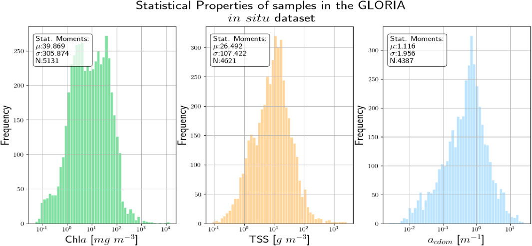
Figure 2. The statistical distribution of the various biogeochemical variables in the GLORIA in situ database.

The spectral coverage was further restricted to spectral bands <724 nm as the 400–724 nm range contains most information content, and both in situ and MSI-derived matchup R_rs data (see Section 2.2) beyond this range (i.e., in the near-infrared; NIR) carry large uncertainties (Pahlevan et al., 2021a), adding noise to subsequent analyses. To further ensure data quality, any spectra in the GLORIA dataset that has been flagged as having issues like (random) noise, sun-glint correction issues (baseline shift), or instrument miscalibrations have eliminated from consideration. The distribution of the values of the different WQIs in the GLORIA dataset, showing the range of conditions covered, is shown in Figure 2. It is important to mention that although GLORIA contains approximately $7500$ samples, not all samples contain in situ measurements for all the WQIs. Therefore, for each specific variable (e.g., Chl $a$), there are about $4000–5000$ labeled samples (as shown in Figure 2A).

The samples in the GLORIA dataset are measured in the best-case scenario, in terms of the techniques used and the measurement environment chosen, etc., and are expected to have a very high SNR (significantly higher than what is seen in satellite datasets). Due to its comparatively high SNR, predictive efforts focused on these datasets are expected to be more successful than when applied to noisier satellite datasets [N.B.: While the samples in the GLORIA dataset are expected to have a higher SNR, it should be noted that these measurements are not error/noise-free. Possible sources of error include random/systematic noise in field instrument measurements, operation errors, non-ideal environmental conditions, and inaccuracies in laboratory based Chla measurements.]. Satellite data which are the primary data source for the application of such models are expected to be significantly noisier but given the paucity of satellite R_rs with collocated measures of the WQI, in situ datasets like GLORIA are being primarily used for model training and evaluation.

2.2 Satellite matchup dataset

As was briefly mentioned in the previous section, while given their widespread availability in situ datasets are primarily used for machine learning model training and validation, these statistics might not be directly transferable to satellite datasets. To track/present the effect of satellite data acquisition on model performance, we also test the model performance on an MSI matchup dataset. The matchup dataset consists of R_rs spectra which are extracted from atmospherically corrected MSI imagery for which near concurrent in situ Chl $a$ and TSS measurements over multiple water bodies were assembled. The images were processed using the Atmospheric Correction for OLI ’lite’ (ACOLITE) $v20220222$ (Vanhellemont and Ruddick, 2021), which is one of the widely used correction methods for MSI imagery (Pahlevan et al., 2022). The measurements for the samples included in this dataset were obtained from various databases across North America. This includes data from the Chesapeake Bay, the Upper Klamath Lake (Oregon), the Great Lakes in the United States, and Lakes Winnipeg and Simcoe in Canada. The water constituent samples were obtained through various methods, including routine state and federal monitoring activities such as field visits and laboratory analyses¹. The lake data were primarily provided by the Environment and Climate Change Canada (ECCC), while the TSS data was sourced from the U.S. Water Quality Portal (WQP)² and the Geological Survey’s National Water Information System³. Water quality measurements were then paired with the closest corresponding satellite measurements at these locations. For each matchup location, spatial constraints were introduced, and only pixels in a 3x3-element window centered on the matchup locations were considered. A matchup location was considered valid if $\ge 5$ pixels in the spatial window were considered valid water pixels (this caused some nearshore matchup locations to be discarded) (Pahlevan et al., 2020; Smith, et al., 2021). The median value of the valid samples in the 3 × 3 matchup box is computed to represent the satellite derived R_rs sample (Werdell and Bailey, 2005). Generally, a +/− $3$ h time window from the satellite overpass was permitted, for coastal matchups, and similar to previous works (Pahlevan et al., 2021b), a same-day overpass was required for inland waters.

2.3 Multispectral and hyperspectral satellite data

Additionally, some well-studied satellite image cubes at both multi- and hyperspectral resolutions were used to provide some qualitative analysis of the model performance for satellite data. We focus on images from the multispectral sensors of the Chesapeake Bay, a large tidal estuary in the U.S. The images were processed using the ACOLITE $v20220222$ (Vanhellemont and Ruddick, 2021) with the same settings as in Saranathan et al. (2023). The Chesapeake Bay image from MSI was acquired on 17 October 2020, and the OLCI image was acquired on November $7^{th},2016$. For HICO, images of two locations, namely, the Chesapeake Bay (September ${20}^{th},2013$) and Lake Erie (September 8th $,2014$) were used for the analysis. The HICO images were atmospherically corrected using the SeaWiFS Data Analysis System (SeaDAS $v\mathrm{7.5.3}$) (Ibrahim et al., 2018) following the same procedure (using the default options) as in Pahlevan et al. (2021b). Of the PRISMA satellite, an image of the turbid waters of Lake Trasimeno, Italy (July $25th,2020$) (Ludovisi and Gaino, 2010; Bresciani et al., 2022) was processed and examined. The PRISMA products for this sensor were downloaded and reprojected using the associated Geometric Lookup Tables (GLT) (Busetto and Ranghetti) to extract necessary information (such as the band centers and full-width half maximums, and Sun and viewing angles) required for atmospheric correction. Following the estimation of these parameters atmospherically corrected pixel R_rs was estimated using the Atmospheric and Topographic Correction (ATCOR v.9.3.0) (Richter and Schläpfer, 2002) technique with the same settings as in O’Shea et al. (2023).

3 Methods

3.1 Algorithms and settings

This subsection will briefly describe the MDN and BNN-MCD models, we briefly describe their underlying theory, architecture, and parameters. We will also describe here the core hyperparameter settings for the two algorithms used in this manuscript.

3.1.1 Mixture Density Networks

The task of inferring target WQIs from R_rs is inherently an inverse problem (Mobley, 1994). This presents a challenge as the relationship between algorithm input (R_rs) and output (WQIs) is not direct and may have multiple feasible solutions (Sydor et al., 2004). Traditional methods struggle to handle this complexity and may result in oversimplified solutions that overlook significant relationships. Mixture Density Networks (MDNs) have emerged as an effective strategy for handling these inverse problems (Pahlevan et al., 2020; Smith et al., 2021). MDNs are capable of outputting probability distributions - specifically a Gaussian Mixture Model (GMM) (Bishop, 1994). Unlike single output estimates from conventional approaches, GMMs describe an entire range of possible outcomes as a probability distribution, which is particularly advantageous for scenarios with multi-modal output distributions. Provided with enough components, GMMs have the capacity to model distributions of arbitrary complexity (Sydor et al., 2004; Defoin-Platel and Chami, 2007).

Mathematically, a MDN estimates the target variable as an explicit distribution conditioned on the input. As described, a MDN models the output distribution as a GMM, as described in Eq. 1:

$\begin{array}{c}p\left(y|\theta \right)={\displaystyle \sum _{j=1}^k}{\pi }_j\hspace{0.25em}{p}_k\left(y\right)where{p}_k=\mathcal{N}\left({\mu }_k,{\mathrm{\Sigma }}_k\right)\\ s.t.\hspace{0.25em}{\pi }_j\hspace{0.25em}>\hspace{0.25em}0\hspace{0.25em}\forall \hspace{0.25em}j;{\displaystyle \sum _{j=1}^k}{\pi }_j=1\end{array}(1)$

where $\theta ={\left\{{\pi }_j,{\mu }_j,{\mathrm{\Sigma }}_j\right\}}_{j=1}^K$, are the parameters corresponding to the GMM, wherein ${\pi }_j$ is the component probability, and ${\mu }_j$ and ${\mathrm{\Sigma }}_j$ are the mean and variance corresponding to each of the individual Gaussian components. During the training phase, the network is optimized using a negative log-likelihood loss function. This loss function is designed to minimize the discrepancy between the MDN-estimated distribution and the true WQI values corresponding to the samples in the training set. Upon training completion, the MDN produces the components of the GMM, as previously described for test samples. The final model estimation is then derived from this probabilistic representation. This approach to model training and application is consistent with methodologies outlined in prior MDN publications (Balasubramanian et al., 2020; Pahlevan et al., 2020; O’Shea et al., 2021; Smith et al., 2021). The point estimate ($\widehat{y}$) derived from the MDN output employs the maximum likelihood principle, meaning that the output corresponds to the mean of the dominant component in the predicted distribution.

The associated MDN uncertainty is shown to be well approximated by the standard deviation of the distribution predicted by the MDN for a specific sample and parameter (Choi et al., 2018). Since the output of the MDN is a GMM, the standard deviation is given by Eq. 2:

${\sigma }_{UNC}=\sqrt{{\displaystyle \sum _{j=1}^K}{\pi }_j{\mathrm{\Sigma }}_j+{\displaystyle \sum _{j=1}^K}{\pi }_j{\parallel {\mu }_j-{\displaystyle \sum _{j=1}^K}{\pi }_k{\mu }_k\parallel }^2}(2)$

Finally, the estimated uncertainty is converted into a percentage value relative to the predicted value (or the final point estimate from the model) according to Eq. 3:

${\sigma }_{UNC}\left(\%\right)=\left(\frac{{\sigma }_{UNC}}{\widehat{y}}\right)\times 100(3)$

Recent work on MDN applications for the Chl a estimation has shown that the estimated uncertainty metric successfully captures the distortion effects in the data such as noisy data, novel test data, and presence of atmospheric distortions in the data (Saranathan et al., 2023).

3.1.2 Bayesian Neural Network based on monte-carlo dropout (BNN-MCD)

Bayesian Neural Networks (BNNs) build upon the architecture of traditional neural networks by integrating probabilistic modeling into each network component such as weights and biases. Since BNN incorporate probabilistic modeling into each step of the network architecture such models can leverage the probabilistic nature of the model output. Since full Bayesian modeling is computationally intractable, one approach for Bayesian approximation of neural networks is the Monte Carlo Dropout (MCD) strategy, as demonstrated by Werther et al. (2022). MCD combines two components: Monte Carlo sampling and the application of dropout to the network weights. The dropout procedure operates by substituting each fixed weight (${\theta }_i$) in the neural network with a binary distribution. This application results in either zero or a determined value (${\theta }_c$) for a neural network connection. Then, dropout is combined with Monte Carlo sampling. With the dropout active the NNs are used to generate $S$ unique predictions for the various WQI from a single test R_rs sample. Each of these $S$ predictions stem from a unique variant of the neural network, corresponding to a specific sample from the network weight constellation. This diverse aggregation of estimates results in a sample set from a probability distribution (see Eq. 4) for each target variable, showcasing the confluence of Monte Carlo sampling and dropout in the MCD approach:

$p\left(y|x,\mathcal{D}\right)=\frac{1}{S}{\displaystyle \sum _{i=1}^S}p\left(y|x,{\theta }_i\right)(4)$

where $\mathrm{x}$ and $\mathcal{D}$ are the test sample and the training data distribution respectively [see Werther et al. (2022) for more details]. A larger value of $S$ leads to a more diverse range of network variants and associated target variable estimates, thus forming a more comprehensive estimation of the statistics associated with the probability distribution but comes at increased computation and time cost. Sampling is then performed from all determined Gaussian distributions $y\sim \mathcal{N}\left({\mu }_x,{\mathrm{\Sigma }}_x\right)$, where ${\mu }_x$ represents the mean of the variable and ${\mathrm{\Sigma }}_x$ stands for its standard deviation. Using the sampling mentioned above creates a set of possible guesses $S_{\mu }=\left[{\mu }_x^1,{\mu }_x^2,....,{\mu }_x^S\right]$, the final estimate $\widehat{y}$ is the mean of the set $S_{\mu }$, while the uncertainty (${\sigma }_{UNC}$) is the standard deviation of the set described above. Again, the estimated uncertainty metric is converted into a percentage as per Eq. 3.

3.1.3 Architecture details and training of the two neural network models

To enable a robust comparison between the two probabilistic NN algorithms described above, efforts were made to ensure all the architectural hyperparameters associated with the model implementation corresponding to each algorithm are kept in common. In keeping with this effort, the base neural network, i.e., the input and hidden layers for both the algorithm models are made the same. The full details of this base neural network are given in Table. 1. The only differences between the two models are in the shape/structure of the output layer and the use of dropout even in the output stage for the BNN-MCD. In terms of data preprocessing, to stay consistent with prior work (Pahlevan et al., 2020; O’Shea et al., 2021; Smith et al., 2021; Saranathan et al., 2023), both the input data (i.e., R_rs) and the output data (WQIs) are scaled to improve model performance. The same pre-processing steps are used in both prediction pipelines. The R_rs data were scaled using a simple inter-quartile range (IQR) scaling to minimize the effect of the outliers. The output parameters (specifically Chl a and TSS) contain values over a very large range (0–1000 mg/m3). To minimize the effects of the larger magnitudes on model performance, we first apply a simple log-scaling. The parameter distributions post-log-scaling are shown in Figure 2 (the x-axis is in the log-scale). Finally, the output variables are also scaled to fit in the range $\left[-1,1\right]$ by using MinMax scaling. Both neural network models are then implemented using Google’s TensorFlow framework (Abadi et al., 2016) and the code is readily available on dedicated repositories (on request).

Table 1

Table 1. The architecture and training hyper-parameters of the Base Neural Network used by both the MDN and BNN-MCD algorithms in this manuscript.

The full prediction pipelines for the two algorithms are shown schematically in Figure 3. As described above both pipelines use the same preprocessing and base neural networks. The main intrinsic model differences are the number of components in the output in each network and the mode in which the output is estimated from the distribution. An additional difference is that for the MDN, ten models are trained, and the output is the median point estimate of the ensemble. The BNN-MCD output is with the MC-Dropout active as mentioned in Section 3.2. In our experiments $S$ was set to $100$, and statistics performed as mentioned above.

Figure 3

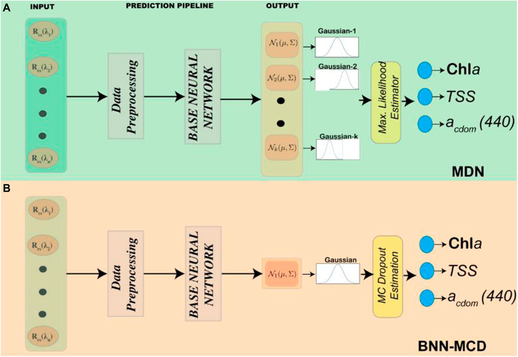
Figure 3. A schematic representation of the full prediction pipeline for the (A) MDN and (B) BNN-MCD, both pipelines leverage the same base neural network defined in Table. 1.

3.2 Evaluation strategies

This subsection outlines the various experiments conducted to analyze the models corresponding to the two probabilistic neural networks. First, we establish the metrics used to evaluate the performance of these models in terms of both predictive residuals and estimated uncertainty (Section. 3.2.1). We then proceed to evaluate the model performances using the GLORIA in situ dataset (Section. 3.2.2). We further gauge the generalization performance of the two models using a leave-one-out approach (Section. 3.2.3), followed by comparing the performance of single-parameter models to that of multi-parameter models (Section. 3.2.4). The final subsection is dedicated to the satellite matchup assessment (Section. 3.2.5).

3.2.1 Evaluation metrics: Predictive performance and uncertainty

The choice of metrics plays a key role in comparing the performance of different models. For the WQI estimation we use a variety of metrics to measure the difference between the true and predicted values referred to as residuals. We thus consider a suite of well-established metrics for measuring predictive (regression) residuals. These metrics are similar to the ones used in previous publications (Seegers et al., 2018; Pahlevan et al., 2020; O’Shea et al., 2021; Smith et al., 2021; Werther et al., 2022), like the Root Mean Squared Log Error ($RMSLE$) and Mean Absolute Error ($MAE$) which are measures of the model’s average residuals in log and linear space respectively. While such average measures are useful to understand the performance over the full dataset, the average operation is affected significantly by outliers. Whereas metrics like Median Symmetric Accuracy ($MdSA$) and Signed Symmetric Percentage Bias ($SSPB$), which contain a median operation are less sensitive to outliers and provide a better estimation of model performance on the bulk of the data. The slope metric provides insight into the correlation between the true and predicted values [For the exact mathematical formulation of the various metrics see Supplementary Appendix SB.].

Additionally, the estimated uncertainties are compared using the following metrics.

1. Sharpness ($\overline{{\sigma }_{UNC}}\left(\%\right)$): The sharpness $\overline{{\sigma }_{UNC}}\left(\%\right)$ defined in Eq. 5 is the median of the uncertainties across all the samples in the test set, from a specific prediction pipeline. The sharpness is defined separately for each product WQI. This metric would provide the user with insights into the (%) uncertainty associated with a typical model prediction for a specific product at a chosen spectral resolution from that dataset. Ideally, one would prefer to have a low value for sharpness, and a value closer to $0$ would indicate that the model is completely confident in its prediction for the specific sample.

$\overline{{\sigma }_{UNC}\left(\%\right)}=Md\left(\left[{\sigma }_{UNC}^1\left(\%\right),{\sigma }_{UNC}^2\left(\%\right)\dots ..,{\sigma }_{UNC}^N\left(\%\right)\right]\right)(5)$

where ${\sigma }_{UNC}^i\left(\%\right)$ represents the uncertainty associated with the $i^{th}$ sample in the test set for a specific WQI.

2. The Coverage Factor (${\rho }_{UNC}$) (%): is designed to gauge how well the estimated uncertainty can serve as a reliable boundary for the prediction error in a test set. Specifically, it checks how often the true value (y) for a sample fall within a range defined by the predicted value $\widehat{y}$ plus or minus the estimated uncertainty (${\sigma }_{UNC}$). The metric (Eq. 6) calculates the percentage of test samples that meet this condition. Ideally, this percentage should be close to 100%, indicating that the estimated uncertainty is an accurate reflection of the prediction error (IOCCG report, 2019) for all samples.

${\rho }_{UNC}=\%\hspace{0.25em}\text{of\hspace{0.17em}samples\hspace{0.17em}such\hspace{0.17em}that\hspace{0.17em}}\widehat{y}-{\sigma }_{UNC}\le y\le \widehat{y}+{\sigma }_{UNC}(6)$

The best-performing models will have simultaneously a low value for sharpness along with a high value for the coverage factor.

3.2.2 Model training and held-out (test) set assessment

The first experiment compares and contrasts the performance of the two algorithms on the labeled GLORIA in situ dataset (see Section 2.1 for details). The performance of the MDN and BNN-MCD are tested for parameter retrievals and uncertainty estimation for the three parameters of interest at the spectral resolution of all four sensors (MSI, OLCI, HICO, and PRISMA). Further, the dataset is divided into two groups using a $50:50$ split to create a training set and a test set. The training set is used for training the models, while the test is only used to validate model performance. Any missing WQIs in the training dataset are imputed by using simple nearest-neighbor imputations (Troyanskaya et al., 2001) [each GLORIA sample (R_rs and WQI) is modeled as a point in high dimensional space and using a nan-Euclidean distance (i.e., any NaN dimensions in either sample are ignored) the nearest neighbors are identified. Any missing values for a specific sample are the average of the specific dimension over the nearest neighbors (ignoring NaNs)] available as part of Python’s scikit-learn distribution (Pedregosa et al., 2011). In this experiment, we chose to use an imputed training set as opposed to filling missing values by a posterior estimation method similar to previous attempts (Pahlevan et al., 2022; O’Shea et al., 2023) to ensure that differences in the posterior estimation methods do not contribute to differences in the performance of the two prediction pipelines. The same training dataset with the missing values filled in is used for training both models. The performance of both models is tested in terms of both parameters as well as uncertainty estimation on the common test set for the specific sensor resolution. Note that no imputations were performed on the test set. Rather, the performance for each WQI was estimated using only the samples in the test set with in situ measurements for the specific WQI. This is the reason the number of samples for each WQI is a different number in the test set (see Table. 3). Further in the manuscript the test set is also referred to as the held-out dataset as these samples are held-out from the training for model validation.

3.2.3 Leave-one-out assessment

The results of the previous $50:50$ held-out experiment offer a reasonable estimation of model performance when the training and test distributions are similar. However, in practical applications, this assumption may not consistently hold. More commonly, an operational model is exposed to samples outside of the training distribution or from new regions, which may include both familiar and novel R_rs. To simulate such a scenario, we conducted several Leave-One-Out (LOO) type experiments, similar to those previously performed by (Werther et al., 2022; O’Shea et al., 2023). GLORIA includes contributions from numerous researchers, labs, and field campaigns. To assess the impact of novel samples, we iteratively trained MDN and BNN-MCD versions by excluding samples from a specific source or field campaign each time (see Table. 2 for details on the individual datasets) and using the rest of the GLORIA database for training. Similar to the previous section, imputation is only carried out on the training samples before training. Further, the samples left-out of training in a specific trial are referred to as the left-out samples for that trial. We then evaluated the models’ performance on samples from the excluded regions (referred to as left-out test set), computing and reporting both predictive performance (using the MdSA metric mentioned in Section. 3.2.1 as the key metric) and estimated uncertainty.

Table 2

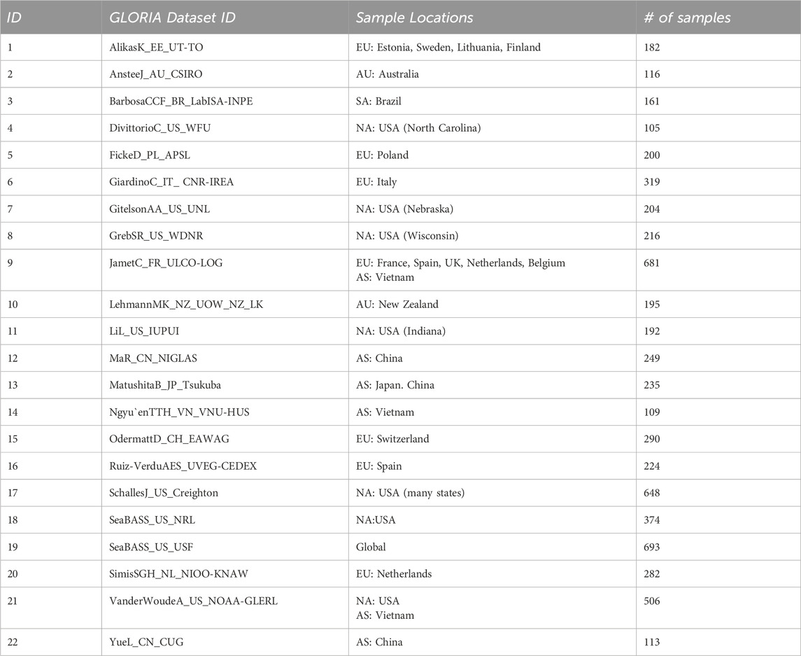
Table 2. The different component subsets of the GLORIA dataset used for Leave-One-Out Validation [N.B.: Column-2 provides the GLORIA dataset IDs for each left out dataset in the analysis.].

It is important to note that some of these data sources contain in situ data from various regions and timeframes (e.g., SeaWiFS Bio-optical Archive and Storage System; SeaBASS). Additionally, not all regions have in situ measurements for all the WQIs considered in this manuscript, which limits our ability to evaluate the algorithm performances for specific indicators within selected datasets. While the LOO approach provides valuable insights into the model’s capacity to handle novel data, it is inherently constrained by the extent of variability captured within the GLORIA dataset. Consequently, when applied globally, this method may encounter locations where the model’s generalization capabilities significantly deviate from those suggested by the GLORIA data. This underscores the potential for encountering performance outliers not adequately represented in the current dataset. Despite these limitations, this LOO analysis is valuable to more accurately assess the individual model’s ability to generalize to unseen data from different geographic locations and water conditions.

3.2.4 Individual retrieval vs. simultaneous retrieval

The comparison of individual (single parameter) versus simultaneous (multi-parameter) retrievals of target variables offers a unique opportunity to better understand the performances and uncertainties associated with the two probabilistic neural network models. Single parameter estimation algorithms (Lee and Carder, 2002; Gitelson et al., 2007), offer precise understanding and interpretability of individual variables while minimizing the complexity introduced by multi-dimensional inter-dependencies. On the other hand, machine learning algorithms are naturally equipped to handle simultaneous retrieval, capitalizing on the inherent correlations and inter-dependencies among multiple variables. This capability offers a nuanced view of aquatic ecosystems by considering the correlations between WQIs. For instance, elevated phytoplankton biomass generally corresponds with increased TSS levels. Conversely, variations in CDOM absorption might not exhibit the same dependencies. Here we investigate the trade-off between the simplicity and interpretability offered by a single-target retrieval and the comprehensive representation of aquatic ecosystems provided by simultaneous estimation. For this purpose, we compare the Chla estimation from a dedicated model, such as those presented previously (Pahlevan et al., 2020; Werther et al., 2022) to the Chl $a$ estimations from multi-parameter models described in Section. 4.2 on the held-out test set, noting that BNN-MCD has previously not been tested for this capacity. This experiment is performed for OLCI’s spectral resolution representing a mid-range spectral capability between multispectral and hyperspectral band settings. This comparison is designed to briefly illuminates the value/effect of such simultaneous retrieval of WQIs for these probabilistic neural network models.

3.2.5 Performance on MSI matchup dataset

The match-up experiment tests and compares the performance of the different algorithms on the satellite matchup data from MSI images described in Section. 2.2. The performance of the models on this dataset would provide the user with some idea of the performance gap that exists when applying these models trained on high quality/low noise in situ datasets to satellite data. Given the additional complexities of the atmospheric correction and residual calibration biases (IOCCG report 2010; Warren et al., 2019), enhanced sensor noise, and distortions present in satellite derived R_rs products, it is expected that the performance of these models on the satellite data will be significantly poorer. The available matchup dataset has corresponding in situ measurements for only Chla and TSS. In this scenario, using the full multiparameter model defined in Sec 3.2.2 is not appropriate as some of the performance gap for this model might be due to the allocation of model capacity to a_cdom (440) estimation. To avoid this issue, we retrain the model using the in situ GLORIA data but using only Chla and TSS as outputs (the rest of the model settings are the same as in Sec. 3.2.2). Post-training, we apply this newly trained dual output model to the matchup data and estimate prediction performance and uncertainty.

4 Results

This section compares and contrasts the results of the two algorithms across the different experiments described in Section. 3.2.

4.1 Held-out assessment

The performance profiles of the two algorithms - MDN and BNN-MCD–in terms of predictive residuals are summarized in Table 3, where the best-performing model for each sensor and metric is highlighted in bold. While the results present a nuanced landscape, some trends do emerge. For instance, the MDN generally outpaces the BNN-MCD in terms of the MdSA metric by approximately 2%–5% across all three WQIs studied. It also exhibits slope values closer to the ideal of 1, albeit by a narrow margin of 1%–2%. Conversely, the BNN-MCD surpasses the MDN in RMSLE by margins of 0.02–0.04 and also shows superior performance in MAE - leading by 5–20 mg m^-3 for Chla and 1–3 g m^-3 for TSS, although it falls behind slightly in estimating a_cdom (440) by about 0.06 m^-1. SSPB performance is more sensor-specific, but it is noteworthy that both models demonstrate a low bias (≤10%) across all WQIs.

Table 3

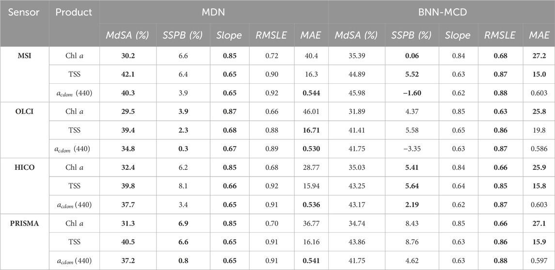
Table 3. Comparison of the performance of the MDN and BNN-MCD across different WQIs for the in situ data at various sensor resolutions. MAE is reported in terms of the physical units of each parameter, i.e., mg m^-3, g m^-3, m^-1 for Chl $a\left(N=2544\right)$, TSS $\left(N=2338\right)$, and $a_{cdom}\left(440\right)\left(N=2228\right)$, respectively. The other metrics are either in % or unitless. The bolded values show the best performance achieved for a specific parameter-sensor combination.

The uncertainty metrics across different WQIs and sensors are summarized in Table. 4. Intriguingly, the MDN generally exhibits lower confidence with sharpness values $\overline{{\sigma }_{UNC}}\left(\%\right)$ ranging from 50% to 60%. In contrast, the BNN-MCD reports notably sharper confidence intervals ($\overline{{\sigma }_{UNC}}\left(\%\right)\sim$ 22-25 $\%$). However, the MDN’s uncertainty estimations appear to align more closely with predictive errors; the prediction error lies within the estimated uncertainty for a substantial portion of samples, as indicated by coverage factors ${\rho }_{UNC}\left(\%\right)$ ranging from 68%–78%. The BNN-MCD, while offering sharper estimates, has a lower rate of agreement between the estimated error and the actual predictive error, reflected by (${\rho }_{UNC}\left(\%\right)$ between approximately $35-48\%$).

Table 4

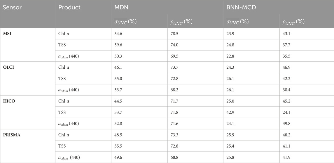
Table 4. Comparison of the different uncertainty metrics for the MDN and BNN-MCD for the different parameters at the resolution of different spectral sensors.

4.2 Leave-one-out assessment

For a large majority of the left-out test sets (∼17-19 out of 22 left out datasets, with the exact number based on the specific WQI) the prediction error (measured using $MdSA$) is higher for both the MDN and the BNN-MCD than error encountered in the 50:50 held-out dataset (top row of each subfigure in Figure 4). These differences indicate the difficulties when extending model application to previously unseen samples. A similar trend is seen in the middle row of each subfigure in Figure 4, which shows the uncertainty/sharpness ($\overline{{\sigma }_{UNC}}\hspace{0.25em}\left(\%\right)$) for the specific parameter estimated by the two models on specific left-out test set. The median sharpness over the LOO sets is shown by the solid line, while the sharpness on the 50:50 held-out set is shown by the dashed lines. It is noteworthy, that in general the left-out sets generally show higher uncertainty (in the form of larger sharpness ($\overline{{\sigma }_{UNC}}\hspace{0.25em}\left(\%\right)$) values for both models). The datasets with the largest uncertainties also show correspondingly higher error, that said the trends are not obvious, further the uncertainty values across the different models are quite comparable. Additional analysis is necessary to illuminate the trends present in these observations.

Figure 4

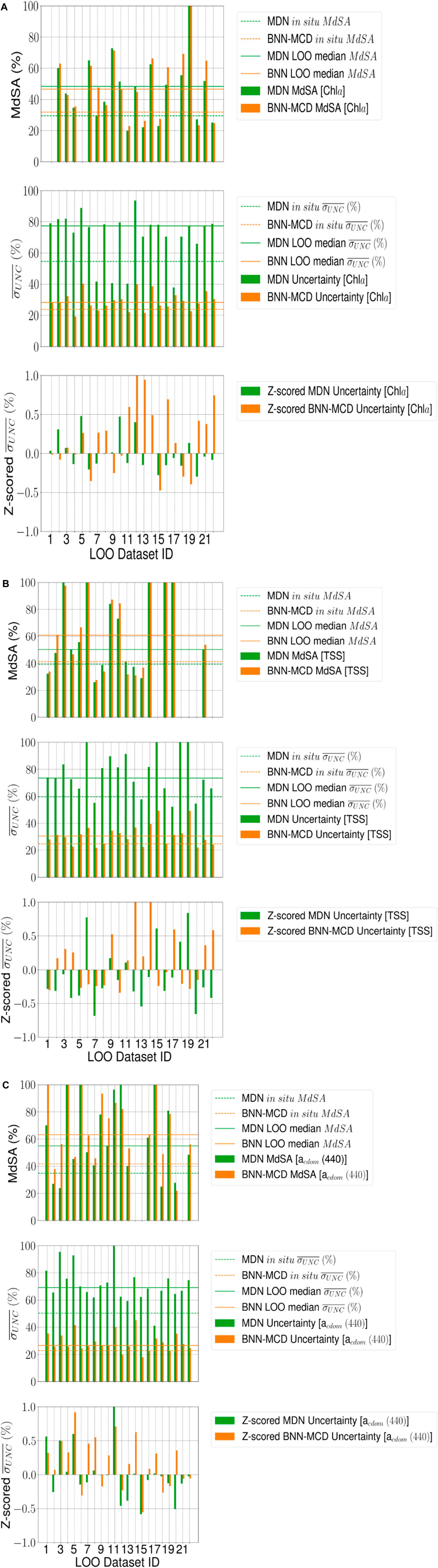
Figure 4. (Continued).

The lack of clarity in uncertainty trends could arise from multiple factors that influence the basic uncertainty metric (${\sigma }_{UNC}\left(\%\right)$). While this metric is partially dependent on the similarity between test and training samples, it is also shaped by extraneous factors such as training data distribution, model hyperparameters, and random initialization, etc. Each model’s training dataset is distinct, complicating cross-model uncertainty comparisons. To mitigate this, we normalize the estimated uncertainties from the left-out test set using the z-score method, based on statistics of the uncertainty metric (${\sigma }_{UNC}\left(\%\right)$ on the training set. This adjusted metric, labeled as z-scored $\overline{{\sigma }_{UNC}}\hspace{0.25em}\left(\%\right)$, offers a clearer relationship with predictive error. For instance, consider Figure 4A middle panel, where two held-out datasets (IDs: 2 & 3) initially exhibit similar uncertainty/sharpness for Chla. Once the z-score normalization is applied to these uncertainties the values are significantly different (see Figure 4A bottom panel). Note that when it is left out, samples in Dataset ID:2 (over Australian waters) exhibit high average uncertainties relative to the samples in the training set, while for Datset ID:3 the average uncertainty is like what is seen for samples in the training sets. As such, we can surmise that for Dataset ID:2 the models are relatively less confident on the left-out set samples, while for Dataset ID:3 the models are as confident on the left-out set samples as training set ones. In summary, the zscore normalization is extremely valuable in highlighting/identifying test samples for which the model is uncertain relative to the standard uncertainty metric which is affected by some bulk factors like the ones mentioned above.

Generally, both models report very similar trends for most datasets across the different WQIs for both MdSA and z-scored $\overline{{\sigma }_{UNC}}\hspace{0.25em}\left(\%\right)$, i.e., high error corresponds to high uncertainty and vice versa. To illuminate these relationship between the $MdSA$ and z-scored $\overline{{\sigma }_{UNC}}\hspace{0.25em}\left(\%\right)$ further, Table 5 reports the ranks (with high ranks for left-out datasets with large error or uncertainty) of predictive error and z-scored $\overline{{\sigma }_{UNC}}\hspace{0.25em}\left(\%\right)$ across the $22$ left-out datasets considered (Table. 2). In most cases, the ranks for the error and uncertainty are comparable. For this discussion, when the ranks of error ($MdSA$) and z-scored $\overline{{\sigma }_{UNC}}\hspace{0.25em}\left(\%\right)$ are within $6$ of each other, we consider them similar/comparable. Table 5 clearly highlights cases wherein the difference between the error and uncertainty ranks are greater than $6$, there are specific cases where the models show high error-low uncertainty (highlighted in red in Table 5) and some held-out datasets with low error-high uncertainty (highlighted in green in Table 5). There is agreement between the two algorithms on the most problematic left-out datasets in terms of the relationship between prediction error to model-estimated uncertainty. The in situ dataset leading to the highest disparity for both ML models is the one comprising of samples from Italian waters (Dataset ID:6 from Giardino, C.). Other instances of datasets with high error and low uncertainty are Dataset ID: 18 (i.e., SeaBASS-NRL for Chla estimation for both algorithms), Dataset ID: 12 (from Ma, R. over Chinese water for ${\mathrm{a}}_{\text{cdom}}$ (440) estimation with both algorithms). Additionally, Dataset IDs: 9 (Chla, ${\mathrm{a}}_{\text{cdom}}$ (440)), 10 (TSS), 15 (TSS), 19 (Chla) have comparatively high error low uncertainty in the BNN-MCD estimation. In addition, there a few cases of low error-high uncertainty wherein in spite of reasonable predictions models are not overly confident. It should be noted that the BNN-MCD results show more examples with mismatch between the error and uncertainty ranking. On a cautionary note, this analysis should not be over-interpreted (in terms of comparing algorithm performance) as significant details are lost when one uses a ranking. Also, the difference chosen as significant in this analysis was arbitrary. Instead, the analysis is only intended to exhibit the general agreement between estimated uncertainty and predictive error on the left-out datasets and in identifying specific datasets/regions where the model generalization is suspect for both algorithms.

Table 5

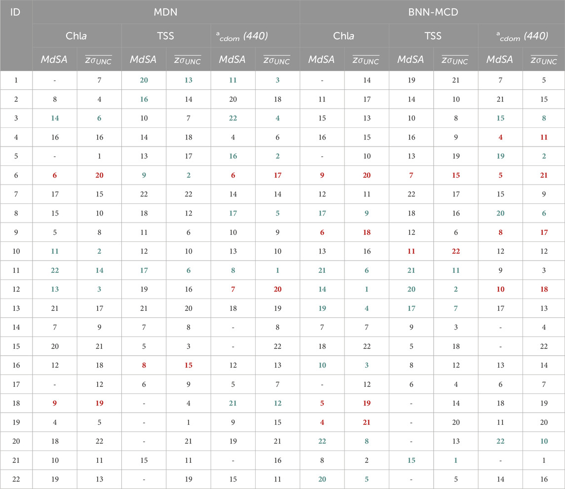
Table 5. Comparing rankings of predictive error (MdSA) and z-scored uncertainty ($\overline{{\sigma }_{UNC}}\hspace{0.25em}\left(\%\right)$) from MDN and BNN-MCD. The cases highlighted in red correspond to “high error low uncertainty cases”, whereas the cases highlighted in green correspond to “low error high uncertainty”.

4.3 Individual retrievals vs. simultaneous retrievals

Overall, the performance of the simultaneous models is slightly better compared to the single-parameter models. Table. 6 shows the effect of the individual (referred to by the label as ‘Base’) versus simultaneous estimation (referred to by the label as ‘Sim’) of Chl $a$ for OLCIs’ spectral resolution. The MDN-Sim model shows upticks across almost all metrics for residual estimation $\left(\sim 1\%MdSA,2\%SSPB,-0.03slope,16.74mg{m}^{-3}MAE\right.$) and the BNN-MCD-Sim shows a similar trend $\left(\sim -0.5\%MdSA,2\%SSPB,0.02slope,6.45mg{m}^{-3}MAE\right.$) [the -ve sign indicates specific metrics where the ‘Base’ model outperforms the ‘Sim’ model]. Cumulatively, these metrics show a general improvement in the quality of the estimations with a simultaneous inversion scheme. Also note that, while both the base models have similar uncertainties (differs only by about $5-7\%$ in terms of $\overline{{\sigma }_{UNC}}\hspace{0.25em}\left(\%\right)$) than the simultaneous models, they significantly underestimate the error for a larger percentage of the samples than the simultaneous models (by $\sim 20\%$ for MDN and $7\%$ for the BNN-MCD), indicating that the simultaneous estimation regularizes models uncertainty by better identifying unexpected data conditions.

Table 6

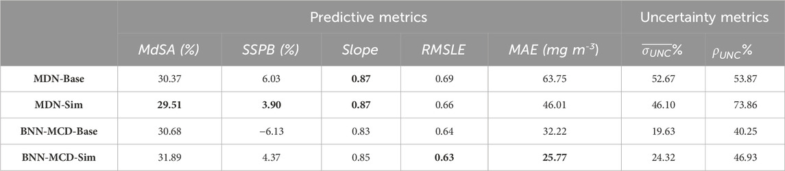
Table 6. Comparison of MDN individual (‘Base’) and simultaneous (‘Sim’) estimators for Chlorophyll-a estimation, both parameter and uncertainty estimations on the held-out test set. MAE is reported in terms of the physical units of the parameter, i.e., mg m⁻³, g m⁻³, m⁻¹ for Chla, TSS, and a_cdom (440), respectively. The other metrics are either (%) or unitless. The bolded cells indicate the best performance of a specific metric.

4.4 MSI matchup assessment

The results of the parameter estimation for the two models on the MSI matchup dataset are shown in Figure 5. Similar to the MDN performance in Pahlevan et al., 2022, there is a rather significant drop-off in performance across the two algorithms relative to the performance we observed on the in situ matchup dataset. For example, $MdSA$ for Chla estimation drops to around $195\%$ from the $30\%$ encountered in the GLORIA dataset. For TSS the drop is not as severe and is between 110% (MDN) and 150% (BNN-MCD) from the ∼42% on the GLORIA dataset. Such degradation in performance is seen across all metrics. The estimated uncertainty metrics on the matchup datasets are shown in Table. 7. While both models show increased uncertainty for Chla (with $\overline{{\sigma }_{UNC}}$ of 72.39% (MDN) and 51.94% (BNN-MCD)) for this dataset relative to the metrics seen in Table 4, the coverage factor for the MDN drops quite significantly (by about 15%), indicating that the increase in uncertainty is not sufficient.

Figure 5

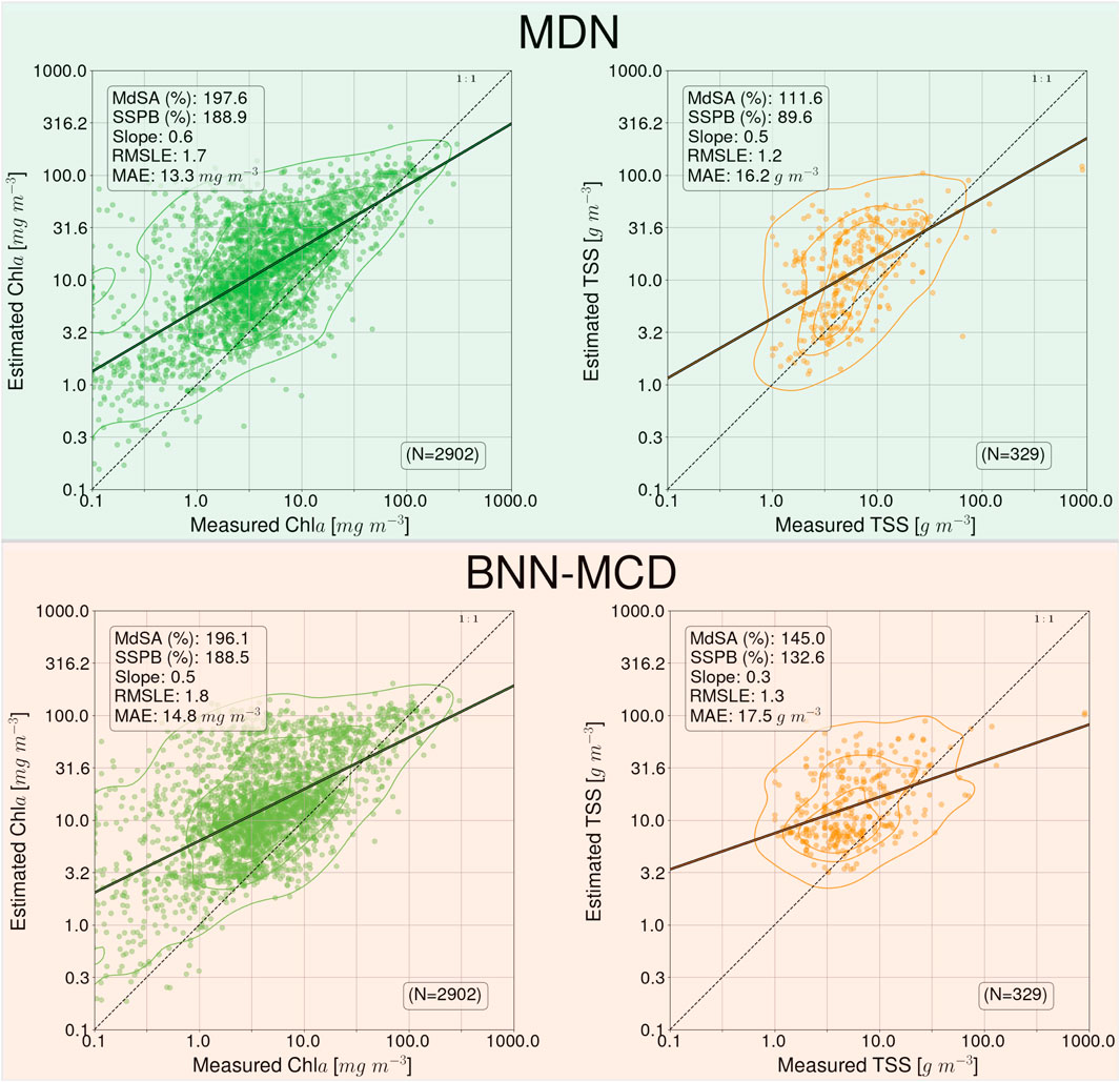
Figure 5. Performance of the MDN and BNN-MCD models for WQI estimation on the ACOLITE corrected MSI matchup dataset.

Table 7

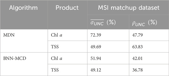
Table 7. Uncertainty estimated by the MDN and BNN-MCD on the ACOLITE corrected MSI matchup dataset.

4.5 Prediction performance on satellite data

This section displays some maps generated by the two models for different satellite datacubes across different missions, at varying spectral resolutions. In particular, WQI and associated uncertainty maps for different multispectral and hyperspectral sensors over the Chesapeake Bay are shown in Figures 6–8. There is general agreement between the spatial trends of WQIs predicted by the two models. Figure 6 shows that the MSI-derived maps from the two models are quite similar for all three parameters, although localized differences in the spatial distributions and magnitudes are occasionally observed. The MDN uncertainty maps seem more uniform, with the BNN-MCD uncertainty exhibiting more spatial variation (note that, in general, the BNN-MCD uncertainty maps capture a broader dynamic range relative to the MDN). In Figure 7, we note some differences, while the spatial trends (i.e., regions with high and low values) are quite similar for the parameters predicted by the two algorithms, there are some differences, with the MDN predictions being slightly lower for Chla and slightly higher for TSS and a_cdom (440) relative to the BNN-MCD predictions. The uncertainty maps for the OLCI cube in Figure 7 also display clearly different trends, indicating that the models are not in concert, as was seen for the MSI images (shown in Figure 6). For the HICO maps of the Chesapeake Bay (shown in Figure 8), there is a clear agreement between the models in the main stem of the bay, however, in the coastal shelves (at the bottom of the image) there are clear disagreements on the predicted values, with BNN-MCD returning high TSS and a_cdom (440) in comparison to those from MDN. These pixels also suffer from high uncertainty (especially for the MDN), indicating rather low confidence in these predictions. The highly elevated uncertainties likely indicate high uncertainties in R_rs products. The HICO acquisition of Lake Erie (see Figure 9) again shows general agreements in terms of predicted parameter values with localized differences in uncertainties. That said, MDN estimates of Chla are generally higher than those of BNN-MCD while its a_cdom (440) predictions are lower. The PRISMA maps of Lake Trasimeno (see Figure 10) for both algorithms continue to show the same general trends, without significant discrepancies in their spatial variability.

Figure 6

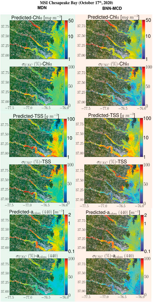
Figure 6. Comparing the MDN (on the left) and BNN-MCD (on the right) estimated parameters and uncertainty for the MSI acquisition of Chesapeake Bay.

Figure 7

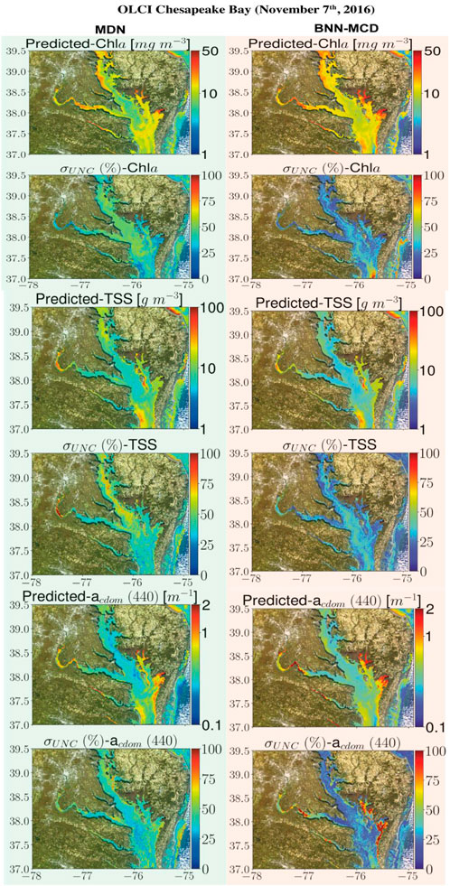
Figure 7. Comparing the MDN (on the left) and BNN-MCD (on right) estimated parameters and uncertainty for the OLCI acquisition of Chesapeake Bay.

Figure 8

Figure 8. Comparing the MDN (on the left) and BNN-MCD (on right) estimated parameters and uncertainty for the HICO acquisition of Chesapeake Bay.

Figure 9

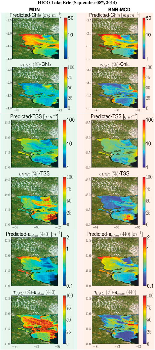
Figure 9. Comparing the MDN (on the left) and BNN-MCD (on right) estimated parameters and uncertainty for the HICO acquisition of Lake Erie.

Figure 10

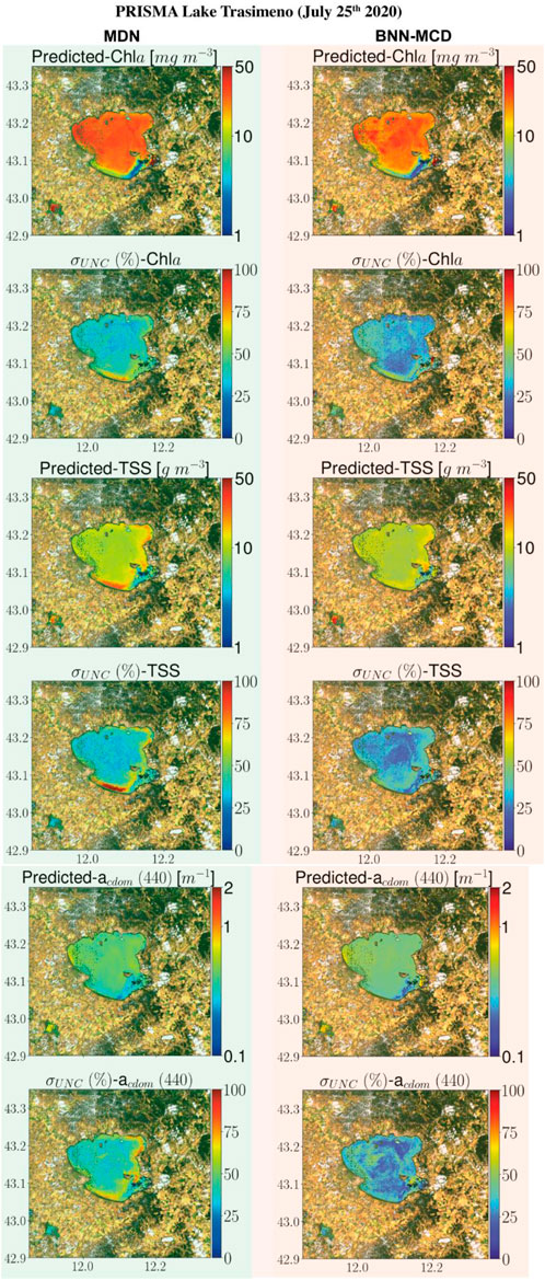
Figure 10. Comparing MDN (on the left) and BNN-MCD (on right) estimated parameters and uncertainty for the PRISMA acquisition of Lake Trasimeno.

5 Discussion

5.1 WQI estimation from spectral samples

Across the different experiments performed in this manuscript it appears that the two probabilistic neural network models have very similar performances in terms of the WQI estimation. On the held-out test dataset the residuals of the two algorithms are very similar across the different sensors and WQIs (see Section 5.1; Table 3 for full results). On the held-out test set the MDN performs better for outlier insensitive $MdSA$ (by 3%–5% across all parameters) and slope (by 0.01–0.03 across all parameters), while the BNN-MCD does better in terms of the outlier-sensitive RMSLE (by 0.03–0.04 for Chla and TSS) and the MAE (by 3–20 mg m^-3 for Chla, 1–3 g m^-3 for TSS), except in the case of a_cdom (440) where the MDN does better (∼0.2 for RMSLE and 0.05 m^-1 for MAE). This observation that the MDN outperforms the BNN-MCD in terms of outlier-insensitive metrics (which use a median operation) while showing poorer performance for the outlier-sensitive metrics (which use a mean operation) indicates that the MDN is generally more accurate but is also more prone to having outliers in its predictions, which exhibit large/extreme errors. It is also worth noting that both models perform better for Chla estimation than the other two WQIs. This difference may be due to the availability of a larger set of labels for this specific WQI. On the other two WQI, the performance of the models is quite similar across most metrics (except MdSA, where there are some differences). In a multivariable learning scenario, the exact losses are also affected by factors such as the precise set of samples in the training set. Further, when these probabilistic models were applied to left-out datasets which contained samples unlike the ones used in training, it becomes clear that in spite of using the GLORIA dataset which attempts to include samples from a variety of different (geographic and aquatic) conditions, there are generalization issues, as most of the left-out datasets (described in Section 3.2.3 and results in Section. 4.2) exhibit a higher error than the error encountered for the held-out test set (described in Section. 3.2.2 and results in Section 4.1). In most cases, these differences are not extreme, however, this observation alludes to the fact that while the GLORIA dataset is a valuable resource and a significant first step, considerable work still needs to be done to create labeled datasets that cover the full distribution of possible water conditions in freshwater and coastal ecosystems and can generalize well to any new test samples. Based on the results in Section 4.3 (especially in Table. 6), one can also infer that across all the different metrics, the best-performing model for the OLCI sensor is one that performs simultaneous estimation rather than a dedicated model. That said, it should also be noted that these gains are quite modest. It is interesting to note that for both models the simultaneous (‘Sim’) estimation causes improvements in the metric wherein the dedicated (‘Base’) model performs worst (RMSLE and MAE for the MDN, slope and MdSA for BNN-MCD), indicating that the simultaneous estimation provides significant regularization (which refers to the set of the set of techniques in ML designed to calibrate the models to fit better on the test set) for the specific model’s predictions.

While the performance of these models is quite impressive when applied to in situ data (even the left-out samples), the performance does not hold up when these models are applied to the satellite matchup datasets. Possible causes for such deterioration could be the imperfect atmospheric correction manifest in satellite-derived R_rs in the form of overcorrection or under-correction of aerosol and water-surface contributions by the atmospheric correction processor. It is also possible the satellite sensors have lower SNR relative to the dedicated sensors used for acquiring the in situ $R_{rs}$ samples.

5.2 Model specific uncertainty estimate

In terms of uncertainty estimation, the main takeaway is that there are fundamental differences in the average uncertainty score per prediction, the MDN is has high uncertainties in the range of around 50% of the predicted value per sample on the held-out test set, while the BNN-MCD appears more confident and shows uncertainties in the range of ∼22% of the predicted value per sample on the held-out test set. While the sharpness estimates (as shown by the BNN-MCD) is preferable, it should be noted that MDN uncertainty is an upper bound on the prediction residual for a much larger fraction of the held-out test set samples (${\rho }_{UNC}\left(\%\right)$ of 68%–75% for MDN vs 45%–50% for BNN-MCD), which would be valuable in using the uncertainty metric to understand the magnitude of the residuals present in the model’s prediction. These results also indicate additional calibration/scaling steps are required to make these uncertainty metrics a better approximation for the kind of errors present in the predictions of these algorithms, to make these products more useful to the end-users.

Similar results are also seen for the raw uncertainty numbers of the LOO experiments, i.e., the BNN-MCD results have a higher sharpness relative to the MDN across all the left-out test sets. The inability of these probabilistic models to generalize to these left-out datasets in terms of predictive performance is also echoed by increases in uncertainty relative to the values seen in the held-out datasets for both probabilistic models. This is encouraging as it indicates that the uncertainty metric can flag the conditions where higher residuals are present. Another observation is that the overall uncertainty (in the form of $\overline{{\sigma }_{UNC}}\hspace{0.25em}\left(\%\right)$) of the left-out datasets seem to be pretty comparable across all datasets. On z-scoring this metric as described in Section. 4.2, the trends become clearer showing a clearer agreement in terms of the ranks of the predictive residuals and uncertainty (see Table. 5 where high error ranks generally correspond to high uncertainty ranks and vice versa), which indicates significant work needs to be done to further resolve the various components going into the uncertainty metrics as defined and further isolate the factors related to predictive performance. While in general there is very good correlation between the residual rankings and uncertainty ranking of the different left out datasets there are specific cases where the rankings do not match. Particularly concerning are the left-out datasets with high residuals and low uncertainty (marked in red in Table 5), as this indicate cases where the uncertainty is not able to tag the presence of high residuals in the predictions.

One such dataset, is the dataset containing samples over Italian waters (Dataset ID: six in Table 2), wherein models face significant issues, and despite poor estimation performance, both models estimate rather low uncertainty for samples in this dataset. Perhaps, some of these issues could be traced back to possible differences in the data acquisition for the samples in this dataset. There are also other examples wherein the models suffer from high errors with disproportionately low uncertainty, but these apply to specific parameters, such as Dataset ID: 18 for Chla estimation, and Dataset ID: 12 for $a_{cdom}$ (440) estimation. In addition, Table. 5 also tracks datasets where models estimate high uncertainty in spite of low prediction errors (highlighted in green). While the uncertainty metric was designed to provide the user with a notion of model confidence in a prediction and possible error, it should be stressed that uncertainty is not a perfect proxy for the error; as such, it cannot be considered incorrect for the model to suggest low confidence for some examples even though they exhibit low estimation error. It is possible that we are able to generate accurate predictions in spite of the model not being exposed to similar samples in training. Further, this scenario is less damaging in downstream processing (than showing low uncertainty for samples with high error), as this will just lead to some additional oversight rather than missing samples with large prediction errors. It is also noted that, in general, the MDN shows fewer examples with significant differences in the levels (in terms of the ranks shown in Table 5) of error and uncertainty. While the ranking scheme described for this experiment is not perfect (Section. 4.2), the MDN uncertainty metric better captures the issues in generalizing to a left-out dataset.

The regularization enabled by simultaneous estimation also has a pronounced impact on the uncertainties. For both models, the concurrent models show significant improvements in the coverage factor ${\rho }_{UNC}\left(\%\right)$ estimated even though the average sharpness $\overline{{\sigma }_{UNC}}\hspace{0.25em}\left(\%\right)$ changes only by $\sim 5\%$. These improvements indicate that the simultaneous estimation forces a clearer understanding of the possible error in the prediction (particularly for the MDN). Finally, on the matchup dataset both models show a significant spike in the prediction uncertainties indicating possible issues in the predictions. That said the coverage factor for both models is quite poor indicating that their approximation of uncertainty on the matchup datasets is poorer than on the in situ datasets considered in previous experiments. This gap indicates more work to be done in future projects to bridge this gap.

The general trend of the MDN poorer average sharpness $\overline{{\sigma }_{UNC}}\hspace{0.25em}\left(\%\right)$ results while having better coverage factor ${\rho }_{UNC}\left(\%\right)$ vis-a-vis the BNN-MCD across many different sensor resolution and experimental conditions is interesting. Perhaps these differences can be traced back to the MDN being designed to consider possible multi-modality in the distributions of the WQI which causes it to consider a wider range of possible values making it more pessimistic, while the unimodal BNN-MCD is more optimistic. The specific properties of each uncertainty metric are property of the specific formulation and may need additional calibration to distill information relevant to the end-users.

5.3 WQI and uncertainty maps on satellite image datasets

The WQI maps (Figures 6–10) offered a qualitative perspective on the sensitivity of the models to uncertainties in input R_rs maps and enabled underscoring similarities and discrepancies for different satellite sensors with varying spectral capabilities. Although similarities exist among the map product estimates, disagreements can be found across the maps. For instance, MDN-derived a_cdom (440) in MSI maps exhibit larger values than those of BNN-MCD on the west stem of the Chesapeake Bay and its tributaries, although the corresponding TSS and Chla maps are generally on par. The largest differences are observed in HICO-derived maps (Figure 8), where BNN-MCD returns higher constituent concentrations and organic content along the main stem of and outside the Chesapeake Bay. Without in situ data sets, it is difficult to offer any insights into the relative accuracy of these products; nonetheless, these product estimates provide evidence of major discrepancies in models’ performance in practical applications, as shown in Figure 5. These observations support the need for comprehensive assessments of future models in real-world applications.

The relative performance of models in uncertainty estimation is generally aligned well with our held-out or LOO analyses (Section. 4.1, 4.2). Of note is that similar to the matchup analyses in Figure 5, pixel uncertainties are >50% (MDN) and >25% (BNN-MCD) for most maps, which is consistent with our observations on the level of uncertainty in the MSI matchup data (Table 7). There are, however, exceptions to this statement where BNN-MCD outputs larger uncertainties at local scales (see MSI and HICO uncertainty maps of Chla in Figures 6, 9). Overall, for reliable use of uncertainty estimates, the most critical aspect of uncertainty estimates is consistency in time and space, an exercise that can be examined in the future.

6 Conclusion

This manuscript provides the first comprehensive comparison of the two state-of-the-art ML algorithms, the MDN and the BNN-MCD, similarly trained, tested, and deployed for data from multiple satellite missions. Model performance was analyzed in terms of both WQI estimates and estimates of associated model-specific uncertainties. The algorithms were tested under similar conditions, such as training data distributions, model architecture, comparison metrics, using various methods, including testing on held-out test sets, tests under a LOO scheme. Overall, we observe that the performance of the two probabilistic neural networks is quite similar across many experiments, such as prediction residuals on the 50:50 held-out test set (∼30–35% for Chla, 45%–50% for TSS, and 40%–45% for a_cdom (440)), and the leave-one-out type experiments (∼40–45% for Chla, 55%–60% for TSS, and 40%–50% for a_cdom (440)). The MDN predictions appear to fit the bulk of the samples well with some outliers, whereas the BNN-MCD predictions have fewer outliers and fit global distribution better. In terms of model-specific uncertainty, the MDN generates higher uncertainties, in general, ∼50% of the predicted values for in situ samples, while the BNN-MCD uncertainties are closer to ∼20–25% of the predicted values. That said, the MDN uncertainty provides better coverage of the error with coverage factors of ∼65–75%, while the corresponding coverage of the BNN-MCD is ∼50%. The LOO experiments also show that for left-out datasets, the ranks of prediction errors and uncertainties are quite comparable (generally between 5-6 ranks of each other). Overall, it appears that these model-specific uncertainty metrics, while capable of flagging/identifying test samples with higher relative residuals, the exact uncertainty values are heavily dependent on model properties, and significant work still needs to be done to calibrate/scale these metrics into easily interpretable quantities of for (e.g., expected prediction residuals) human interpretation.

Another, important contribution of this manuscript is the validation of effect of simultaneous estimation on the performance of these machine learning models. For this purpose, the BNN-MCD was also extended into the simultaneous estimation paradigm, and both models were tested in this scheme against a dedicated single-parameter (Chla) estimator. It is noted that the simultaneous WQI retrieval outperforms individual retrieval and displays improvements across most of the regression residuals considered in this project. Additionally, while the uncertainty metrics do not appear to show massive changes in the average sharpness there are clear improvements in the coverage of the estimated uncertainty values. Both models were also tested on the satellite matchup datasets to provide some insight into the performance when these models were applied to satellite-derived $R_{rs}$. In this case also we noted that application of models trained on high fidelity in situ datasets exhibit a significant degradation when applied to nosier satellite test samples. Finally, maps were produced on satellite datasets to provide a qualitative comparison and validation of satellite-derived products.

Future research should aim to broaden the comparison between MDNs and BNN-MCDs by introducing other probabilistic modeling techniques. This expansion will provide more nuanced insights into the interplay between training data and model type. Additionally, recalibration techniques like Platt scaling (Platt, 1999) or Isotonic regression (Barlow and Brunk, 1972) can be employed to refine the model-specific uncertainty estimates, potentially mitigating some of the limitations identified in this study concerning predictive uncertainty. A further promising avenue is to employ labeled samples to devise a mapping between estimated uncertainties and actual predictive errors. Another important avenue of research in the uncertainty estimation would be the combination of the different data and physical sources along with ML-model based uncertainty to get a comprehensive metric for the expected residual in the final prediction/estimate. For this purpose, we are considering the use Monte Carlo (MC) sampling-based techniques (Kroese et al., 2013) that can be used to propagate uncertainties from different operations like atmospheric correction, elimination of adjacency effects, down to downstream products like WQI estimates (Zhang, 2021).

Data availability statement

Publicly available datasets were analyzed in this study. The GLORIA dataset can be found here: https://doi.pangaea.de/10.1594/PANGAEA.948492.

Author contributions

AS: Data Curation, Formal Analysis, Investigation, Methodology, Software, Validation, Visualization, Writing–original draft, Writing–review and editing, MW: Formal Analysis, Methodology, Investigation, Writing–original draft, Writing–review and editing. SB: Data Curation, Methodology, Writing–review and editing. DO: Supervision, Funding Acquisition, Resources, Writing–review and editing. NP: Conceptualization, Supervision, Funding Acquisition, Resources, Writing–review and editing.

Funding

The author(s) declare that financial support was received for the research, authorship, and/or publication of this article. This work was supported in part by the National Aeronautics and Space Administration (NASA) Research Opportunities in Space and Earth Sensing (ROSES) under grants 80NSSC20M0235 and 80NSSC21K0499 associated with the Phytoplankton, Aerosol, Cloud, Ocean Ecosystem (PACE) Science and Applications Team and the Ocean Biology and Biogeochemistry (OBB) program, respectively. This work was also supported by the Swiss National Science Foundation scientific exchange grant number IZSEZ0_217542 and grant Lake3P number 204783. PRISMA 953 Products^© of the Italian Space Agency (ASI) used in the experiments was delivered under an ASI License to use.

Acknowledgments

We also acknowledge the public in situ databases as part of NOAA’s Great Lakes monitoring program, the Chesapeake Bay Program, and their 946 partners.

Conflict of interest

Authors AS and NP were employed by Science Systems and Applications, Inc.

The remaining authors declare that the research was conducted in the absence of any commercial or financial relationships that could be construed as a potential conflict of interest.

The author(s) declared that they were an editorial board member of Frontiers, at the time of submission. This had no impact on the peer review process and the final decision.

Publisher’s note

All claims expressed in this article are solely those of the authors and do not necessarily represent those of their affiliated organizations, or those of the publisher, the editors and the reviewers. Any product that may be evaluated in this article, or claim that may be made by its manufacturer, is not guaranteed or endorsed by the publisher.

Supplementary material

The Supplementary Material for this article can be found online at: https://www.frontiersin.org/articles/10.3389/frsen.2024.1383147/full#supplementary-material

Footnotes

¹https://www.canada.ca/en/environment-climate-change/services/freshwater-quality-monitoring/online-data.htm

²https://www.waterqualitydata.us

³https://nwis.waterdata.usgs.gov/nwis

References

Abadi, M., Agarwal, A., Barham, P., Brevdo, E., Chen, Z., Craig, C., et al. (2016). Tensorflow: large-scale machine learning on heterogeneous distributed systems. arXiv Preprint arXiv:1603.04467.

Google Scholar

Balasubramanian, S. V., Pahlevan, N., Smith, B., Binding, C., Schalles, J., Loisel, H., et al. (2020). Robust algorithm for estimating total suspended solids (TSS) in inland and nearshore coastal waters. Remote Sens. Environ. 246, 111768. doi:10.1016/j.rse.2020.111768

CrossRef Full Text | Google Scholar

Barlow, R. E., and Brunk, H. D. (1972). The isotonic regression problem and its dual. J. Am. Stat. Assoc. 67 (337), p140–p147. doi:10.2307/2284712

CrossRef Full Text | Google Scholar

Bishop, C. M. (1994). Mixture density networks.

Google Scholar

Bresciani, M., Giardino, C., Fabbretto, A., Pellegrino, A., Mangano, S., Free, G., et al. (2022). Application of new hyperspectral sensors in the remote sensing of aquatic ecosystem health: exploiting PRISMA and DESIS for four Italian lakes. Resources 11 (2), 8. doi:10.3390/resources11020008

CrossRef Full Text | Google Scholar

Busetto, L., and Ranghetti, L. (2021). Prismaread: a tool for facilitating access and analysis of PRISMA L1/L2 hyperspectral imagery V1. 0.0. 2020. Available Online: Lbusett. Github. Io/Prismaread/.

Google Scholar

Candela, L., Formaro, R., Guarini, R., Loizzo, R., Longo, F., and Varacalli, G. (2016). “The PRISMA mission,” in 2016 IEEE international geoscience and remote sensing symposium (IGARSS) (IEEE), 253–256.

CrossRef Full Text | Google Scholar

Cao, Z., Ma, R., Duan, H., Pahlevan, N., Melack, J., Shen, M., et al. (2020). A machine learning approach to estimate chlorophyll-a from landsat-8 measurements in inland lakes. Remote Sens. Environ. 248, 111974. doi:10.1016/j.rse.2020.111974

CrossRef Full Text | Google Scholar

Castagna, A., and Vanhellemont, Q. (2022). Sensor-agnostic adjacency correction in the frequency domain: application to retrieve water-leaving radiance from small lakes. doi:10.13140/RG.2.2.35743.02723

CrossRef Full Text | Google Scholar

Choi, S., Lee, K., Lim, S., and Oh, S. (2018). “Uncertainty-aware learning from demonstration using mixture density networks with sampling-free variance modeling,” in 2018 IEEE international conference on robotics and automation (ICRA) (IEEE), 6915–6922.

CrossRef Full Text | Google Scholar

Defoin-Platel, M., and Chami, M. (2007). How ambiguous is the inverse problem of ocean color in coastal waters? J. Geophys. Res. Oceans 112 (C3). doi:10.1029/2006jc003847

CrossRef Full Text | Google Scholar

Drusch, M., Bello, U. D., Carlier, S., Colin, O., Fernandez, V., Gascon, F., et al. (2012). Sentinel-2: ESA’s optical high-resolution mission for GMES operational services. Remote Sens. Environ. 120, 25–36. doi:10.1016/j.rse.2011.11.026

CrossRef Full Text | Google Scholar

Gilerson, A., Herrera-Estrella, E., Foster, R., Agagliate, J., Hu, C., Ibrahim, A., et al. (2022). Determining the primary sources of uncertainty in retrieval of marine remote sensing reflectance from satellite ocean color sensors. Front. Remote Sens. 3, 857530. doi:10.3389/frsen.2022.857530

CrossRef Full Text | Google Scholar

Gilerson, A. A., Gitelson, A. A., Zhou, J., Gurlin, D., Moses, W., Ioannou, I., et al. (2010). Algorithms for remote estimation of chlorophyll-a in coastal and inland waters using red and near infrared bands. Opt. Express 18 (23), 24109–24125. doi:10.1364/oe.18.024109

PubMed Abstract | CrossRef Full Text | Google Scholar

Gitelson, A. A., Schalles, J. F., and Hladik, C. M. (2007). Remote chlorophyll-a retrieval in turbid, productive estuaries: Chesapeake Bay case study. Remote Sens. Environ. 109 (4), p464–p472. doi:10.1016/j.rse.2007.01.016

CrossRef Full Text | Google Scholar

Gons, H. J., Rijkeboer, M., and Ruddick, K. G. (2002). A chlorophyll-retrieval algorithm for satellite imagery (medium resolution imaging spectrometer) of inland and coastal waters. J. Plankton Res. 24 (9), 947–951. doi:10.1093/plankt/24.9.947

CrossRef Full Text | Google Scholar

IOCCG (2018). Earth observations in support of global water quality monitoring. Editors S. Greb, A. Dekker, and C. Binding (Dartmouth, NS, Canada: International Ocean-Colour Coordinating Group (IOCCG)), –125pp. (Reports of the International Ocean-Colour Coordinating Group, No. 17). doi:10.25607/OBP-113

CrossRef Full Text | Google Scholar

Gross, L., Thiria, S., Frouin, R., and Mitchell, B. G. (2000). Artificial neural networks for modeling the transfer function between marine reflectance and phytoplankton pigment concentration. J. Geophys. Res. Oceans 105 (C2), 3483–3495. doi:10.1029/1999jc900278

CrossRef Full Text | Google Scholar

Ibrahim, A., Franz, B., Ahmad, Z., Healy, R., Knobelspiesse, K., Gao, B.-C., et al. (2018). Atmospheric correction for hyperspectral ocean color retrieval with application to the hyperspectral imager for the Coastal Ocean (HICO). Remote Sens. Environ. 204, 60–75. doi:10.1016/j.rse.2017.10.041

CrossRef Full Text | Google Scholar

Ioannou, I., Gilerson, A., Gross, B., Moshary, F., and Ahmed, S. (2011). Neural network approach to retrieve the inherent optical properties of the Ocean from observations of MODIS. Appl. Opt. 50 (19), 3168–3186. doi:10.1364/ao.50.003168

PubMed Abstract | CrossRef Full Text | Google Scholar

IOCCG (2000). “Remote sensing of Ocean Colour in coastal, and other optically-complex, waters,” in International Ocean Colour coordinating group: dartmouth, Canada.

Google Scholar

IOCCG (2010). “Atmospheric correction for remotely-sensed ocean-colour products,” in IOCCG reports series, international Ocean Colour coordinating group: dartmouth, Canada.

Google Scholar

IOCCG (2019). “Uncertainties in Ocean Colour remote sensing,” in International Ocean Colour coordinating group. Editor F. Mélin (Canada: Dartmouth).

Google Scholar

Jackson, T., Sathyendranath, S., and Mélin, F. (2017). An improved optical classification scheme for the Ocean Colour Essential Climate Variable and its applications. Remote Sens. Environ. 203, 152–161. doi:10.1016/j.rse.2017.03.036

CrossRef Full Text | Google Scholar

Jamet, C., Loisel, H., and Dessailly, D. (2012). Retrieval of the spectral diffuse attenuation coefficientK_<i>d</i>(λ) in open and coastal ocean waters using a neural network inversion. J. Geophys. Res. Oceans 117 (C10). doi:10.1029/2012jc008076

CrossRef Full Text | Google Scholar

Kajiyama, T., D’Alimonte, D., and Zibordi, G. (2018). Algorithms merging for the determination of Chlorophyll-${a}$ concentration in the black sea. IEEE Geoscience Remote Sens. Lett. 16 (5), 677–681. doi:10.1109/lgrs.2018.2883539

CrossRef Full Text | Google Scholar

Kroese, D. P., Taimre, T., and Botev, Z. I. (2013). Handbook of Monte Carlo methods. John Wiley and Sons.

Google Scholar

Kwiatkowska, E. J., and Fargion, G. S. (2003). Application of machine-learning techniques toward the creation of a consistent and calibrated global chlorophyll concentration baseline dataset using remotely sensed ocean color data. IEEE Trans. Geoscience Remote Sens. 41 (12), 2844–2860. doi:10.1109/tgrs.2003.818016

CrossRef Full Text | Google Scholar

Lee, Z., and Carder, K. L. (2002). Effect of spectral band numbers on the retrieval of water column and bottom properties from ocean color data. Appl. Opt. 41 (12), 2191–2201. doi:10.1364/ao.41.002191

PubMed Abstract | CrossRef Full Text | Google Scholar

Lehmann, M. K., Gurlin, D., Pahlevan, N., Alikas, K., Anstee, J., Balasubramanian, S. V., et al. (2023). Gloria - a globally representative hyperspectral in situ dataset for optical sensing of water quality. Scientific Data in press.

Google Scholar

Liu, X., Steele, C., Simis, S., Warren, M., Tyler, A., Spyrakos, E., et al. (2021). Retrieval of Chlorophyll-a concentration and associated product uncertainty in optically diverse lakes and reservoirs. Remote Sens. Environ. 267, 112710. doi:10.1016/j.rse.2021.112710

CrossRef Full Text | Google Scholar

Lucke, R. L., Corson, M., McGlothlin, N. R., Butcher, S. D., Wood, D. L., Korwan, D. R., et al. (2011). Hyperspectral imager for the Coastal Ocean: instrument description and first images. Appl. Opt. 50 (11), 1501–1516. doi:10.1364/ao.50.001501

PubMed Abstract | CrossRef Full Text | Google Scholar

Ludovisi, A., and Gaino, E. (2010). Meteorological and water quality changes in Lake Trasimeno (umbria, Italy) during the last fifty years. J. Limnol. 69 (1), 174. doi:10.4081/jlimnol.2010.174

CrossRef Full Text | Google Scholar

Maritorena, S., Siegel, D. A., and Peterson, A. R. (2002). Optimization of a semianalytical ocean color model for global-scale applications. Appl. Opt. 41 (15), 2705–2714. doi:10.1364/ao.41.002705

PubMed Abstract | CrossRef Full Text | Google Scholar

Michalak, A. M. (2016). Study role of climate change in extreme threats to water quality. Nature 535 (7612), 349–350. doi:10.1038/535349a

PubMed Abstract | CrossRef Full Text | Google Scholar

Mittenzwey, K.-H., Ullrich, S., Gitelson, A. A., and Kondratiev, K. Y. (1992). Determination of chlorophyll a of inland waters on the basis of spectral reflectance. Limnol. Oceanogr. 37 (1), 147–149. doi:10.4319/lo.1992.37.1.0147

CrossRef Full Text | Google Scholar

Mobley, C. D. (1994). Light and water: radiative transfer in natural waters. (No Title).

Google Scholar

Mobley, C. D. (1999). Estimation of the remote-sensing reflectance from above-surface measurements. Appl. Opt. 38 (36), 7442–7455. doi:10.1364/ao.38.007442

PubMed Abstract | CrossRef Full Text | Google Scholar

Moore, T. S., Dowell, M. D., Bradt, S., and Ruiz Verdu, A. (2014). An optical water type framework for selecting and blending retrievals from bio-optical algorithms in lakes and coastal waters. Remote Sens. Environ. 143, 97–111. doi:10.1016/j.rse.2013.11.021

PubMed Abstract | CrossRef Full Text | Google Scholar

Moses, W. J., Sterckx, S., Montes, M. J., De Keukelaere, L., and Knaeps, E. (2017). Atmospheric correction for inland waters, in bio-optical modeling and remote sensing of inland waters. Elsevier, 69–100.

CrossRef Full Text | Google Scholar

Neil, C., Spyrakos, E., Hunter, P. D., and Tyler, A. N. (2019). A global approach for chlorophyll-a retrieval across optically complex inland waters based on optical water types. Remote Sens. Environ. 229, 159–178. doi:10.1016/j.rse.2019.04.027

CrossRef Full Text | Google Scholar

Nieke, J., Mavrocordatos, C., Craig, D., Berruti, B., Garnier, T., Riti, J.-B., et al. (2015). “Ocean and Land color imager on sentinel-3,” in Optical payloads for space missions (Chichester, UK: John Wiley and Sons, Ltd), 223–245.

CrossRef Full Text | Google Scholar

Odermatt, D., Kiselev, S., Heege, T., Kneubühler, M., and Itten, K. (2008). “Adjacency effect considerations and air/water constituent retrieval for Lake Constance,” in 2nd MERIS/AATSR workshop. Frascati, Italy. University of Zurich, 1–8. 22 September 2008 - 26 September 2008.

Google Scholar

O’Reilly, J. E., Maritorena, S., Mitchell, B. G., Siegel, D. A., Carder, K. L., Garver, S. A., et al. (1998). Ocean color chlorophyll algorithms for SeaWiFS. J. Geophys. Res. Oceans 103 (C11), 24937–24953. doi:10.1029/98jc02160

CrossRef Full Text | Google Scholar

Pahlevan, N., Mangin, A., Balasubramanian, S. V., Smith, B., Alikas, K., Arai, K., et al. (2021a). ACIX-aqua: a global assessment of atmospheric correction methods for landsat-8 and sentinel-2 over lakes, rivers, and coastal waters. Remote Sens. Environ. 258, 112366. doi:10.1016/j.rse.2021.112366

CrossRef Full Text | Google Scholar

Pahlevan, N., Smith, B., Alikas, K., Anstee, J., Barbosa, C., Binding, C., et al. (2022). Simultaneous retrieval of selected optical water quality indicators from landsat-8, sentinel-2, and sentinel-3. Remote Sens. Environ. 270, 112860. doi:10.1016/j.rse.2021.112860

CrossRef Full Text | Google Scholar

Pahlevan, N., Smith, B., Binding, C., Gurlin, D., Lin, Li, Bresciani, M., et al. (2021b). Hyperspectral retrievals of phytoplankton absorption and chlorophyll-a in inland and nearshore coastal waters. Remote Sens. Environ. 253, 112200. doi:10.1016/j.rse.2020.112200

CrossRef Full Text | Google Scholar

Pahlevan, N., Smith, B., Schalles, J., Binding, C., Cao, Z., Ma, R., et al. (2020). Seamless retrievals of chlorophyll-a from sentinel-2 (MSI) and sentinel-3 (OLCI) in inland and coastal waters: a machine-learning approach. Remote Sens. Environ. 240, 111604. doi:10.1016/j.rse.2019.111604

CrossRef Full Text | Google Scholar

Pedregosa, F., Varoquaux, G., Gramfort, A., Michel, V., Thirion, B., Grisel, O., et al. (2011). Scikit-learn: machine learning in Python. J. Mach. Learn. Res. 12, 2825–2830.

Google Scholar

Platt, J. (1999). Probabilistic outputs for support vector machines and comparisons to regularized likelihood methods. Adv. large margin Classif. 10 (3), 61–74.

Google Scholar

Reynolds, N., Blake, A. S., Guertault, L., and Nelson, N. G. (2023). Satellite and in situ cyanobacteria monitoring: understanding the impact of monitoring frequency on management decisions. J. Hydrology 619, 129278. doi:10.1016/j.jhydrol.2023.129278

CrossRef Full Text | Google Scholar

Richter, R., and Schläpfer, D. (2002). Geo-atmospheric processing of airborne imaging spectrometry data. Part 2: atmospheric/topographic correction. Int. J. Remote Sens. 23 (13), 2631–2649. doi:10.1080/01431160110115834

CrossRef Full Text | Google Scholar

Sanders, L. C., Schott, J. R., and Raqueño, R. (2001). A VNIR/SWIR atmospheric correction algorithm for hyperspectral imagery with adjacency effect. Remote Sens. Environ. 78 (3), 252–263. doi:10.1016/s0034-4257(01)00219-x

CrossRef Full Text | Google Scholar

Saranathan, A. M., Smith, B., and Pahlevan, N. (2023). Per-pixel uncertainty quantification and reporting for satellite-derived chlorophyll-a estimates via mixture density networks. IEEE Trans. Geoscience Remote Sens. 61, 1–18. doi:10.1109/tgrs.2023.3234465

CrossRef Full Text | Google Scholar

Schiller, H., and Doerffer, R. (1999). Neural network for emulation of an inverse model operational derivation of case II water properties from MERIS data. Int. J. Remote Sens. 20 (9), 1735–1746. doi:10.1080/014311699212443

CrossRef Full Text | Google Scholar

Seegers, B. N., Stumpf, R. P., Schaeffer, B. A., Loftin, K. A., and Werdell, P. J. (2018). Performance metrics for the assessment of satellite data products: an ocean color case study. Opt. Express 26 (6), 7404–7422. doi:10.1364/oe.26.007404

PubMed Abstract | CrossRef Full Text | Google Scholar

Shea, O., Ryan, E., Pahlevan, N., Smith, B., Boss, E., Gurlin, D., et al. (2023). A hyperspectral inversion framework for estimating absorbing inherent optical properties and biogeochemical parameters in inland and coastal waters. Remote Sens. Environ. 295, 113706. doi:10.1016/j.rse.2023.113706

CrossRef Full Text | Google Scholar

Shea, O., Ryan, E., Pahlevan, N., Smith, B., Bresciani, M., Todd, E., et al. (2021). Advancing cyanobacteria biomass estimation from hyperspectral observations: demonstrations with HICO and PRISMA imagery. Remote Sens. Environ. 266, 112693. doi:10.1016/j.rse.2021.112693

CrossRef Full Text | Google Scholar

Siegel, D. A., Behrenfeld, M. J., Maritorena, S., McClain, C. R., Antoine, D., Bailey, S. W., et al. (2013). Regional to global assessments of phytoplankton dynamics from the SeaWiFS mission. Remote Sens. Environ. 135, 77–91. doi:10.1016/j.rse.2013.03.025

CrossRef Full Text | Google Scholar

Smith, B., Pahlevan, N., Schalles, J., Ruberg, S., Errera, R., Ma, R., et al. (2021). A chlorophyll-a algorithm for landsat-8 based on mixture density networks. Front. Remote Sens. 1, 623678. doi:10.3389/frsen.2020.623678

CrossRef Full Text | Google Scholar

Spyrakos, E., O'donnell, R., Hunter, P. D., Miller, C., Scott, M., Simis, S. G. H., et al. (2018). Optical types of inland and coastal waters. Limnol. Oceanogr. 63 (2), 846–870. doi:10.1002/lno.10674

CrossRef Full Text | Google Scholar

Sydor, M., Gould, R. W., Arnone, R. A., Haltrin, V. I., and Goode, W. (2004). Uniqueness in remote sensing of the inherent optical properties of ocean water. Appl. Opt. 43 (10), 2156–2162. doi:10.1364/ao.43.002156

PubMed Abstract | CrossRef Full Text | Google Scholar

Troyanskaya, O., Cantor, M., Sherlock, G., Brown, P., Hastie, T., Tibshirani, R., et al. (2001). Missing value estimation methods for DNA microarrays. Bioinformatics 17 (6), 520–525. doi:10.1093/bioinformatics/17.6.520

PubMed Abstract | CrossRef Full Text | Google Scholar

Vanhellemont, Q., and Ruddick, K. (2021). Atmospheric correction of sentinel-3/OLCI data for mapping of suspended particulate matter and chlorophyll-a concentration in Belgian turbid coastal waters. Remote Sens. Environ. 256, 112284. doi:10.1016/j.rse.2021.112284

CrossRef Full Text | Google Scholar

Vilas, L. G., Spyrakos, E., and Palenzuela, J. M. T. (2011). Neural network estimation of chlorophyll a from MERIS full resolution data for the coastal waters of Galician rias (NW Spain). Remote Sens. Environ. 115 (2), 524–535. doi:10.1016/j.rse.2010.09.021

CrossRef Full Text | Google Scholar

Wang, M., and Gordon, H. R. (1994). Radiance reflected from the Ocean–atmosphere System: synthesis from individual components of the aerosol size distribution. Appl. Opt. 33 (30), 7088–7095. doi:10.1364/ao.33.007088

PubMed Abstract | CrossRef Full Text | Google Scholar

Warren, M. A., Simis, S. G. H., Martinez-Vicente, V., Poser, K., Bresciani, M., Alikas, K., et al. (2019). Assessment of atmospheric correction algorithms for the sentinel-2A MultiSpectral imager over coastal and inland waters. Remote Sens. Environ. 225, 267–289. doi:10.1016/j.rse.2019.03.018

CrossRef Full Text | Google Scholar

Werdell, J. P., and Bailey, S. (2005). An improved in-situ bio-optical data set for ocean color algorithm development and satellite data product validation. Remote Sens. Environ. 98 (1), 122–140. doi:10.1016/j.rse.2005.07.001

CrossRef Full Text | Google Scholar

Werther, M., and Burggraaff, O. (2023). Dive into the unknown: embracing uncertainty to advance aquatic remote sensing. J. Remote Sens. 3. doi:10.34133/remotesensing.0070

CrossRef Full Text | Google Scholar

Werther, M., Odermatt, D., Simis, S. G. H., Gurlin, D., Lehmann, M. K., Kutser, T., et al. (2022). A bayesian approach for remote sensing of chlorophyll-a and associated retrieval uncertainty in oligotrophic and mesotrophic lakes. Remote Sens. Environ. 283, 113295. doi:10.1016/j.rse.2022.113295

CrossRef Full Text | Google Scholar

Zhang, J. (2021). Modern Monte Carlo methods for efficient uncertainty quantification and propagation: a survey. Wiley Interdiscip. Rev. Comput. Stat. 13 (5), e1539. doi:10.1002/wics.1539

CrossRef Full Text | Google Scholar