Selecting HyperNav deployment sites for calibrating and validating PACE ocean color observations

A novel ocean profiling float system for calibrating and validating satellite-based ocean color observations has been developed and tested. The float-based radiometric sampling system, herein referred to as HyperNav, is complementary to traditional moored in-situ observing systems and provides additional capability due to the relatively small platform size and high radiometric accuracy that allows for opportunistic deployments at locations during seasons and conditions that are best for ocean color observations. The purpose of this study is to optimize the deployment locations of an array of HyperNav systems to support the Plankton, Aerosol, Cloud, ocean Ecosystem (PACE) mission by performing System Vicarious Calibration (SVC) observations. Specifically, we present the development of logistical and scientific criteria for selecting suitable sites for developing an SVC network of profiling-float-based radiometric systems capable of calibrating and validating ocean color observations. As part of the analyses described in this paper, we have synthetically deployed HyperNav at potential US-based and international sites, including: north of Crete island; south-east of Bermuda island; south of Puerto Rico island; southwest of Port Hueneme, CA; west of Monterey, CA; west of Kona, HI; and south-west of Tahiti island. The synthetic analyses identified Kona, Puerto Rico, Crete, and Tahiti as promising SVC sites. All sites considered are suitable for generating a significant number of validation match-ups. Optimally deploying HyperNav systems at these sites during the PACE post-launch SVC campaign is expected to cost-effectively provide a large number of SVC match-ups to fulfill the PACE calibration requirements.

1 Introduction

For over 40 years, observations from ocean color satellites have inferred surface ocean biogeochemistry on an unprecedented spatial and temporal scale. These data have been important in understanding many of the grand challenges of our age, such as marine pollution, the global marine food web, and global carbon cycles (Groom et al., 2019; Brewin et al., 2023). Reflected sunlight entering the satellite’s field of view comes mostly from atmospheric sources and only a small fraction is reflected from within the ocean. The subtleties of ocean color interpretation depend on the accuracy of the retrieved ocean color signals and, therefore, also the accuracy of the atmospheric correction methods used to obtain these data (Gilerson et al., 2022). As such, correction schemes require that Earth-orbiting ocean color satellites be well calibrated, with known and quantified uncertainties, to obtain precise ocean color radiance spectra with a known accuracy. (Franz et al., 2007; McClain and Meister, 2012; Bisson et al., 2021).

Satellites are calibrated through a combination of pre- and post-launch observations using well-characterized optical targets. Post-launch characterizations of satellite-borne measurements are dependent on signal response for known and well-specified (i.e., lowest uncertainty) oceanic signals in a process known as system vicarious calibration (SVC). Vicarious calibration systems are observational platforms dedicated to collecting in-situ observations that can be compared to satellite ocean color data for calibration. The SVC component of satellite calibration is considered critical to reach the high accuracy necessary to make meaningful ocean color observations (Frouin et al., 2013; Johson et al., 2024). Plankton, Aerosol, Cloud, ocean Ecosystem (PACE) satellite, lauchched on February 6, 2024, carries an Ocean Color Instrument (OCI) capable of resolving reflected ocean light at 5 nm resolution spanning from the UV to the visible and into NIR spectrum and promises to transform our understanding and monitoring of phytoplankton communities and ocean biogeochemistry (Frouin et al., 2019; Werdell et al., 2019). Observations on such a fine spectral scale require substantial calibration and validation efforts to be of known uncertainty and, hence, utility.

Historically, in-situ SVC observations have been collected from two specially designed and equipped moorings: the Marine Optical Buoy (MOBY) mooring (Clark et al., 1997) located off the island of Lanai in the Hawaiian island chain, and the now decommissioned Bouée pour l’acquisition de Séries Optiques à Long Terme (BOUSSOLE) mooring (Antoine et al., 2006) located off the coast of Villefranche-sur-Mer in Southern France. The MOBY and BOUSSOLE moorings have successfully recorded over 20 years of SVC quality observations (Valente et al., 2016) and MOBY remains a critical component of any SVC array. Moorings typically record high-frequency observations at one geographical location over a long time series. These data are useful for long-term inter-calibration and resolving complex time-varying signals, but are poorly suited for resolving large spatial variability. Moorings are expensive and could be difficult to maintain: mooring equipment typically requires complicated shipping and logistics to mobilize; moorings typically require large ships to assemble and place; and surface sensors can quickly foul with biological organisms, which require regular cleaning and maintenance. Another potential limitation is that moored sensors typically collect data at fixed depths, whereas optical profiles can resolve stratification details.

The Argo semi-Lagrangian profiling float (Roemmich et al., 2019) is a complementary platform to moorings and ship-based hydrography. Core Argo floats are typically deployed from ships, then drift at 1,000 m and ascend to the surface once every 10 days to broadcast their collected temperature and salinity profiles. Argo floats only have buoyancy control and are advected by ocean currents. Argo floats are relatively low cost and are typically analyzed in concert over a large array to resolve spatial variability. There are now over 3,800 Argo floats deployed in all the world’s oceans. The distributed Core Argo array complemented by targeted moorings has improved our understanding of difficult problems such as ocean currents, steric height, and heat content (Miller, 1990; Servain et al., 1998; Wong et al., 2020).

Since its original introduction, the Argo platform has been modified to carry additional sensors. The HyperNav sensor (Barnard et al., 2022) is an Argo float-borne optical sensor specifically designed for satellite SVC operations. HyperNav typically samples once per day ($\approx$ local noon time), has a relatively small form factor, can be shipped via cargo plane, is easily deployed from a small fishing or utility boat, and costs an order of magnitude less than a comparable mooring. A distributed array of HyperNav systems, like Argo, can sample larger spatial variability than moorings alone and may reduce unexplained biases in satellite-based ocean color (Bisson et al., 2021).

Argo floats executing their standard mission can drift substantial distances over their lifetime (Chamberlain et al., 2023). SVC match-up site locations are carefully chosen to maximize the quality of SVC observations. To maximize the utility of radiometer-equipped floats for SVC match-ups and to recover the sensors for post-calibration, floats should remain in the general vicinity of the original deployment location. To accomplish this, we have devised a novel float navigation method that uses predictions of ocean currents to compute future float displacement at different drift depths. An operator can then transmit optimized mission programming to the float that adjusts the float drift depth to achieve some degree of control over position based on the structure of the ocean currents. Identifying these locations can be done using high-resolution computer simulations.

The flexibility of the HyperNav system, as well as the spatial and temporal variability in atmospheric and oceanic optical properties, motivates the construction of a distributed SVC system. SVC criteria are stringent (Zibordi et al., 2015; Zibordi and Mélin, 2017) and dependent on environmental factors, such as wind speed and aerosol optical thickness, which are seasonally variable. Consequently, the optimal distribution and timing of HyperNav deployments are not obvious but have the possibility to substantially improve the effectiveness of the array. In this publication, we attempt to optimize such a distributed system by evaluating the number of SVC and validation match-ups as well as estimating the number of match-ups per dollar spent on operations at different sites. Here SVC match-ups are calculated using two criteria: the published Zibordi and Mélin (2017) criteria, and a new criteria described and justified in this publication. We also compute a simpler, validation-specific, clear sky criteria.

We first detail the SVC match-up and validation match-up requirements in Section 2, then in Section 3, we describe the HyperNav observing system. In Section 4, we describe the criteria for optimization: a high likelihood of SVC quality match-ups, economical and easy logistics for operations, and the ability to effectively navigate the float by using ocean currents. Finally, in Sections 5 and 6 we present and discuss the results of our optimization.

2 System vicarious calibration and validation requirements

System Vicarious Calibration (SVC), originally developed for the Coastal Zone Colour Scanner (CZCS) (Gordon, 1987; Evans and Gordon, 1994), consists of comparing retrievals of water-leaving radiance to in-situ measurements at the time of satellite overpass and adjusting the calibration coefficients to force agreement between retrieved and measured quantities. This strategy aims at reducing uncertainties of post-launch radiometric calibration techniques, which are not sufficiently accurate for scientific applications, and biases in atmospheric correction. It has been employed operationally for the processing of imagery from major satellite ocean-color missions (Franz et al., 2007; Frouin et al., 2013).

The suitable SVC sites must satisfy specific and rather strict criteria (Gordon, 1998; Fougnie et al., 1999; Frouin et al., 2013; Zibordi et al., 2015; Zibordi and Mélin, 2017). Firstly, the aerosols should be mostly of maritime origin or at most weakly absorbing with optical thickness below 0.1 in the near-infrared (i.e., very clear atmosphere), and the ocean surface free of whitecaps. In such situations, molecular scattering is the dominant process affecting the top-of-atmosphere (TOA) radiance in the ultraviolet and visible, reducing the impact of uncertainties associated with the atmospheric correction scheme. Selecting situations with little-absorbing aerosols is important because the ensemble of aerosol models to choose from in the operational schemes for atmospheric correction (Ahmad et al., 2010) only includes those aerosol types (i.e., single scattering albedo, ${\omega }_{\mathit{aer}}>$ 0.95 at 440 nm). Secondly, the water-leaving radiance should be uniform over several pixels, and the spatial contrast should be minimal over a distance of about 10 km (Santer and Schmechtig, 2000) to minimize adjacency effects. This generally excludes coastal regions, where aerosols are likely to be absorbing and abundant, spatial variability in water-leaving radiance may be large, and the proximity of land exerts a significant influence on the TOA signal. Furthermore, the sites should experience low cloudiness (to maximize the number of high-quality match-ups) and exhibit low bio-optical complexity (e.g., to properly model/correct bidirectional effects in water-leaving radiance). Another desirable quality is high temporal stability in water and atmosphere optical properties (to minimize atmospheric correction uncertainties), especially when the satellite imagery and the in-situ data are not acquired simultaneously. Oligotrophic waters tend to meet these requirements better than productive waters, despite the water signal exerting a greated influence on the measured TOA radiance in the visible and ultraviolet. This advantage is attributed to their enhanced stability, which minimizes the impacts of satellite spatial resolution and time differences in match-ups. Employing several sites in SVC ensures a more comprehensive, robust, and globally applicable calibration process for satellite ocean color sensors, addressing the challenges associated with the inherent variability of marine environments (Bisson et al., 2021).

The MOBY site in the North Pacific (Clark et al., 2003) and the now decommissioned BOUSSOLE site in the Ligurian Sea (Antoine et al., 2008) have the desired SVC attributes (Gordon, 1998; Zibordi et al., 2015). The operational SVC of current satellite ocean-color sensors has been essentially based on water-leaving radiance data acquired at those two sites. Fougnie et al. (2002, 2010), Zibordi and Mélin (2017), and Kwiatkowska et al. (2022) considered other oceanic sites that have potential for SVC. The focus was on analyzing time series of satellite-derived remote-sensing reflectance, $R_{rs}$, chlorophyll concentration, Chl, diffuse attenuation coefficient at 490 nm, $K_d(490)$, and aerosol optical thickness, ${\tau }_{\mathit{aer}}$, and Ångström coefficient, $\alpha$, according to criteria on magnitude, spatial homogeneity, and temporal stability. Suitable regions were identified in various oceans, especially in the north and southeast Pacific Ocean, the Mediterranean Sea, and the eastern Indian Ocean accompanied by the best-recommended period during the year. Zibordi and Mélin (2017) concluded that the MOBY and BOUSSOLE sites are superior for likely high-quality match-ups but suggested that the Eastern Mediterranean Sea near Crete should be considered as a further SVC site. Kwiatkowska et al. (2022) recommended two sites for Copernicus SVC infrastructure located near El Hierro (Canary Islands, Spain) and Crete (Greece). Note that there is currently no consensus in the published literature regarding the specific selection criteria for SVC. For example, Zibordi and Mélin (2017) used $\alpha <$1, but Kwiatkowska et al. (2022) did not use $\alpha$ restrictions.

Given the above, multi-year L2 satellite imagery of aerosol and surface variables were systematically analyzed in potentially suitable regions to generate a climatology with spatial and temporal variability characteristics. This allowed one to select, using complementary information about trajectory statistics and logistics considerations, the best sites for operational SVC activities using HyperNav systems. The lack of community consensus on SVC match-up criteria and the multitude of potential applications for the HyperNav data motivated the analysis of two different match-up criteria for SVC: first, the previously advanced Zibordi and Mélin (2017) criteria; second, the new criteria advanced herein.

The new criteria are similar yet somewhat different from those of previous analyses: (1) the site should be free of clouds, as well as the ${5\text{\hspace{0.17em}km}}^2\times {5\text{\hspace{0.17em}km}}^2$ area centered on the target pixel, to minimize adjacency effects (based on Bailey and Werdell, 2006); (2) the site should be in open Case 1 waters Morel and Prieur (1977), to minimize water complexity and land influence: (3) wind speed should be $<$8 ${\mathrm{m}\mathrm{s}}^{-1}$, to minimize whitecaps; (4) the coefficient of variation of $R_{rs}$ in the blue (e.g., 443 nm); over a ${3\text{\hspace{0.17em}km}}^2\times {3\text{\hspace{0.17em}km}}^2$ area should be $<$20%, to reduce the impact of time differences between satellite and in-situ measurements, (5) ${\tau }_{\alpha er}$ should be $<$0.1 in the near infrared (e.g., 869 nm), to lessen aerosol influence, and (6) ${\omega }_{\mathit{aer}}$ at 550 nm should be $>$0.95, to remove moderately to strongly absorbing aerosols. Note that a restriction on $\alpha$ ($\alpha <$ 1) would not eliminate dust-type aerosols since they may exhibit values much less than unity - Dubovik et al. (2002) demonstrates $\alpha$ values of 0.4. Such aerosols are relatively frequent over the Mediterranean Sea and off the Atlantic coast of Northern Africa (Saharan dust events). Asian dust is also transported to the Hawaiian islands, with strong influxes during spring (Parrington et al., 1983).

In the following analysis, no constraints were placed on the Sun zenith angle and Chl (all investigated sites were in low latitude Case 1 waters). Results on the potential number of match-ups may differ depending on the satellite mission and time of overpass (e.g., cloudiness may vary with the time of day), as reported by Zibordi and Mélin (2017). We only considered MODIS-Aqua in the statistical analysis (1:30 p.m. equatorial crossing, similar to the upcoming PACE). Therefore, the findings may not be readily generalized to other missions but should nonetheless give a good indication of the expected match-ups for planning SVC activities and the expected match-up for validation at those sites.

For validation purposes, the aforementioned SVC restrictions can be relaxed as long as the satellite retrievals exist (i.e., are not masked), which may exclude pixels contaminated by Sun glint and high aerosol loadings or located too close to land and clouds in other words, pixels for which the atmospheric correction fails (Bailey and Werdell, 2006). To evaluate the suitability of sites for validation (less stringent criteria), we choose only the clear sky condition used for SVC; however, it should be noted that ocean variability may still pose challenges for validation.

3 HyperNav concept

The HyperNav system was designed to address the next-generation of satellite ocean color imagers, including near-continuous hyper-spectral coverage from the near UV to NIR bands, specifically focused on meeting the SVC needs for the PACE mission and the OCI. The HyperNav system includes 2 independent upwelling radiance sensors, each providing 2.2 nm wavelength resolution across the 350 to 900 nm spectral range. The HyperNav system also includes a 4-channel above-water downwelling irradiance sensor. Additional measurements from the HyperNav sensor system include pressure and tilt of the platform. The HyperNav system has two modes of operation: a free-fall sampling mode and an autonomous profiling float integration. For an in-depth description of the HyperNav system, see Barnard et al., 2024a; Barnard et al., 2024b, this volume. This paper focuses on using the HyperNav integrated with an autonomous profiling float equipped with a sensors for temperature, salinity and depth. We briefly describe a typical profiling sequence of the HyperNav system. The profile sequence includes the following phases: descent, park, profile phase, surface hold, and transmission. The descent phase typically occurs after initial deployment or surface transmission. During this phase, an onboard buoyancy engine negatively ballasts the float, and the float sinks to a desired drift depth. The HyperNav system cannot communicate with shoreside researchers once it leaves the surface. The desired drift depth is programmed via transmitted instruction while the float is at the surface. Once the HyperNav system reaches its desired drift depth, the buoyancy engine neutrally ballasts the HyperNav system, and the HyperNav system enters the park phase. In the park phase, the HyperNav float system drifts at depth in low power mode. The ballast system positively ballasts the HyperNav system at a programmed time, and the profile phase starts. During the profile phase, the HyperNav system ascends through the water column while collecting data for surface transmission. A typical mission sequence is to have the float profile once per day, with the HyperNav radiance sensor data collection concentrated in the upper 20 m, including a surface acquisition period. After the profile and surface acquisition is completed, the data is telemetered to shore-side systems using an Iridium satellite connection. Note that the daily data transmission of the HyperNav sensors can take up to 2 h (depending on satellite coverage). The float receives new mission files from shore-side systems, powers down the HyperNav sensor systems, and descends to the set park depth.

4 Selection of HyperNav deployment sites

The primary objective of the HyperNav mission is to generate a substantial volume of high-quality SVC data at minimal cost. Nevertheless, HyperNav systems are also engineered for the validation of satellite-derived water-leaving radiance (or remote sensing reflectance), which necessitates less stringent criteria regarding atmosphere, surface, and water conditions—essentially requiring clear skies over a limited pixel area. Both ocean and atmospheric conditions are dynamic, impacting the feasibility of SVC or validation match-up criteria. However, certain locations during specific seasons are more likely to align with SVC match-up criteria than others (Zibordi and Mélin, 2017). Additionally, the operational costs vary across deployment sites, with factors such as shipping expenses and boat rentals contributing to disparities.

This poses a fundamental optimization question: what is the best spatio-temporal deployment configuration to maximize the number of SVC match-ups and minimize deployment costs? To answer this question, we consider the likelihood of a deployment site meeting the SVC match-up criteria derived from the ocean color record (Section 4.1) in addition to the cost of operations at a site (Section 4.2). Finally, because the floats are not actively propelled laterally, we quantify the navigability of the current structure of each site and, if required, impose additional logistical expenses for small boat operations to reposition a float during a typical deployment of 60 days (Section 4.3).

4.1 Analysis of atmospheric and surface variables

The Zibordi and Mélin (2017) and herein described match-up criteria were calculated from atmospheric and oceanic variables. Ten years of level-1a MODIS-A images (from 1/1/2010 to 12/31/2019) covering the areas of interest were downloaded from the OBPG website (https://oceancolor.gsfc.nasa.gov) and were processed into level-2 data including chlorophyll-a concentration (Chl-a), aerosol optical thickness at 869 nm, and wind speed using l2gen in SeaDAS. Specifically, the wind speed is originally from the National Centers for Environmental Prediction (NCEP) reanalysis dataset with 1° spatial resolution and 6 h temporal resolution. As one of the ancillary data used in l2gen, wind speed is interpolated to MODIS resolution. The level-2 MODIS-A images were first remapped to a 1.1 km equal-area grid and then remapped to a Plate Carrée (equal-angle) grid with 1.1 km resolution at the equator. The remapping algorithm is exactly the one used by NASA OBPG to generate level-3 binned ocean color products (Campbell et al., 1996). Nearest neighbor interpolation was used to fill missing pixels at the edges. Daily single scattering albedo was extracted and computed from the $\mathrm{0.5}°\times \mathrm{0.625}°$ MERRA-2 hourly data for the same time period and interpolated to the binned MODIS grid. The clear sky, Zibordi and Mélin (2017), and herein described SVC match-up probabilities were computed for each month from the year 2010–2019. The clear sky probability is defined as the number of days with valid Chl-a values (hence clear days) in an entire ${\mathrm{5}\mathrm{k}\mathrm{m}}^2\times {\mathrm{5}\mathrm{k}\mathrm{m}}^2$ window divided by the total number of days in each month. The herein described SVC criteria probability is defined similarly but with more criteria, i.e., clear sky, aerosol optical thickness at 869 nm $<$0.1, single scattering albedo $>$0.95, coefficient of variation of $R_{rs}<$0.2 over a ${\mathrm{3}\mathrm{k}\mathrm{m}}^2\times {\mathrm{3}\mathrm{k}\mathrm{m}}^2$ area, and wind speed $<$8 ${\mathrm{m}\mathrm{s}}^{-1}$. match-up probabilities. (Figure 1) illustrates these probabilities for August off Kona, Hawaii, depicting values that reach up to 40% in certain areas.

Figure 1

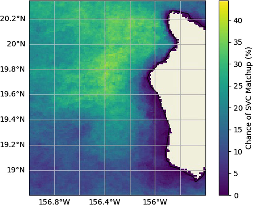
Figure 1. Example of conditional SVC match-up probabilities for an August Kona deployment. Colored shading represents the % chance of an SVC match-up. Beige masking represents land.

4.2 Logistics

For the HyperNav project, the assembly and calibration of the HyperNav system are done at Sea-Bird Scientific in Bellevue, WA, and shipping logistics are staged out of Oregon State University in Corvallis, OR. The cost to mobilize logistics around the world is not uniform and needs to be estimated.

Some sites (Crete, Puerto Rico, Port Hueneme) are in close proximity to advanced oceanographic laboratories operated by collaborators willing to perform float deployments, recoveries, and even in-field equipment refreshes. All other sites require more extensive mobilization: first, the HyperNav system has to be shipped from the Pacific Northwest to the site; next, a team of at least two people is needed at the site to assemble and test the system, arrange deployment logistics and perform the deployment; after the mission is complete, this process must be done in reverse. The sites considered in this manuscript range in travel distance from a long day’s drive to multi-leg international flights across oceans and the differences in logistics costs for float operations between one site and another can be substantial.

To quantify these differences in logistical cost, a simple model was created with information based on previous shipping, daily charter boat rates, and government travel per-diems combined with university overhead (Table 1). We also amortize HyperNav system costs in our deployment cost model. The statistics of HyperNav systems reaching a failure mode after deployments are yet to be determined by our limited number of test deployments; as such, we make the conservative assumption that one float will be lost for every eight deployments (to date one float was lost out of 14 deployments).

Table 1

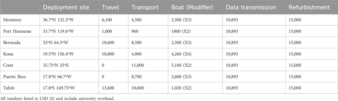
Table 1. Mission deployment and costing information for each deployment site considered. Travel includes round trip transportation and lodging for two people to and from deployment site. Transport includes mobilization logistics for HyperNav system. Boat fee is the daily fee for chartered vessel, fuel, and captain. Modifier is the expected number of boat trips each deployment will require (calculated in Section 4.3.2). Data Transmission includes all iridium satellite transmission fees. Refurbishment includes all replacement batteries and sensor re-calibration. Note that local collaborators in Crete and Puerto Rico eliminate travel costs by generously participating in recovery and deployment operations.

4.3 Navigability

The HyperNav system, like all drifting floats, is advected by ocean currents. HyperNav is a variant of the Argo platform, and, without intervention, this advection can cause substantial displacements from the original deployment location over time (Chamberlain et al., 2023). If the HyperNav system leaves the deployment area, it can be problematic for two reasons: first, the deployment sites are chosen for specific atmospheric and ocean optical properties that are conducive for SVC match-up criteria as described in Section 4.1, therefore HyperNav systems that stay in the deployment area are likely to record more SVC match-up observations than those that leave; second, because of the expense of the system and the time of shipping and assembly, the HyperNav project can deploy in more places and collect more data if the floats are recovered after deployment. Float recovery is much easier if the float stays in the deployment area. Also, HyperNav sensors must be post-calibrated to assess uncertainties in the radiometric measurements over the deployment duration. Currently, without post-calibration, the data collected are not considered of sufficient quality for SVC.

The Argo platform is only propelled in the vertical direction and cannot directly relocate itself laterally. Floats can be picked up and repositioned via a small boat, but this can be costly and logistically complicated to do frequently. The strategy for float piloting that we have adopted in this project is directly analogous to that of aeronauts piloting hot air balloons. Substantial vertical changes in current direction and magnitude exist in the ocean. With sufficient prior knowledge of the structure of the currents, the vertical position of a float can be adjusted such that the float moves in the desired direction.

Predictive high-resolution current models (described in Section 4.3.1) have been operationally combined with the open source Probably A Really Computationally Efficient Lagrangian Simulator (PARCELS) (Lange and van Sebille, 2017) software package to replicate the HyperNav system’s behavior and predict its displacement in near real-time. PARCELS is designed around a flexible and modular architecture compatible with many ocean circulation models and can simulate particle behaviors. PARCELS solves the equations of particle motions using a fourth-order Runge–Kutta scheme. PARCELS particles are programmed to simulate the HyperNav mission by sinking to a predefined drift depth and waiting there for a predetermined period of time (typically 1–5 days), then ascending through the water column and waiting at the surface for 2 h to simulate data transmission before descending again. Vertical velocities in both ascent and descent are 0.076 ${\mathrm{m}\mathrm{s}}^{-1}$, which is typical of a HyperNav in a fully ballasted or de-ballasted state.

This software has been combined with reanalysis models to gain intuition for the best deployment locations and how a float will behave prior to deployment, as well as predictive current models to dynamically adjust HyperNav drift depths and navigate the system during deployment. The code for our calculations is publicly available (https://github.com/Chamberpain/HyperNav), and details of the predictive skill of this novel system will be described in a future publication. Other computational schemes have predicted Argo trajectories or adapted drift depths to navigate floats (Siiriä et al., 2019; González Santana et al., 2023), but this is the first open-ocean, global adaptive navigation system we are aware of.

4.3.1 Model data

Output from four different models are used to simulate float trajectories. These models were of the highest perceived regional skill for each selected site: 1. Output from the Global Ocean Physics Analysis and Forecast (GOPAF) hosted by Copernicus Marine Service and run on the Nucleous for European Modelling of the Ocean (NEMO) (Escudier et al., 2021) model was used for the Crete island, Tahiti, and Bermuda float trajectory predictions, 2. the Mediterranean Sea Physics Analysis and Forecast (MSPAF) also hosted by Copernicus Marine Service and run on the NEMO model was used for Mediterranean simulations. 3. The Pacific Islands Ocean Observing System (PACIOOS) (Powell, 2018) model output was used for the Kona, HI float trajectory predictions, and 4. The Global Ocean Forecasting System (GOFS) run on the HYbrid Coordinate Ocean Model (HYCOM)(Chassignet et al., 2009; Wallcraft et al., 2009) and the Navy Coupled Ocean Data Assimilation (NCODA) system (Cummings and Smedstad, 2014) was used for all other locations (Figure 2).

Figure 2

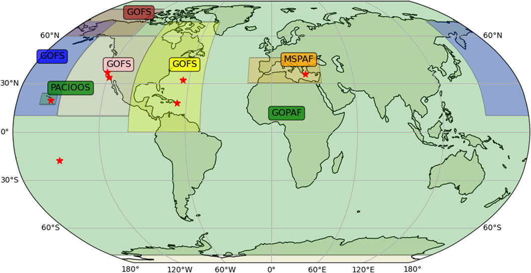
Figure 2. Map of regional extent of currently integrated ocean current models. Shaded regions represent coverage area by each model (see Section 4.3.1 for model descriptions). Red stars indicate study regions.

The MSPAF is a regional model that covers the Mediterranean Sea. The MSPAF has a horizontal grid spacing of 1/24$°$ and 141 vertical levels (Escudier et al., 2021). MSPAF output has hourly resolution. Relatively high vertical resolution is necessary to capture the complicated vertical dynamics present in the Mediterranean, but are unnecessary for our application and were subsampled to 63 levels.

PACIOOS is a Regional Ocean Modeling System (ROMS) based data assimilating model with approximately 4 km grid spacing. Ocean boundary conditions are provided by HYCOM. 6 days predictions are made using assimilated data from PacIOOS high-frequency radars, Argo floats, autonomous underwater vehicles (AUVs), and satellite-based estimates of sea surface height and sea surface temperature. The subsampled model contains 18 depth levels with 3 h output.

GOFS is a hybrid isopycnal-sigma-pressure assimilating model with global coverage. The HYCOM prediction is generated by the US Naval Oceanographic Office and hosted by the National Oceanographic and Atmospheric Administration’s National Centers for Environmental Information. The subsampled model dataset has 30 depth levels, approximately a 1/12° grid cell spacing, and 3 h output.

4.3.2 Navigation test

To quantify the navigability of each site, and ultimately the cost of logistics for repositioning unnavigable floats, we quantified how close we could keep floats to their deployment sites by trying to navigate an ensemble of synthetic floats through hypothetical missions using reanalysis current data from each location. The trajectory prediction computation was described in Section 4.3.

Synthetic floats were initialized at deployment sites selected for a high probability of SVC match-ups as described in Section 4.1. For each profile, future trajectories were calculated for eight drift depths ranging from 50 to 700 m and five drift durations ranging from 1 to 6 days in 1-day increments. The combination of drift depth and drift duration that resulted in the final trajectory location closest to the original deployment location was identified as optimal and the drift depth-duration calculation was repeated for the next profile. Each mission consisted of 60 profiles. Figure 3 shows an example mission off the coast of Kona, HI and illustrates that the optimal drift depth can change many times throughout a deployment. A Monte Carlo simulation conducted these synthetic missions at twenty random deployment times at each deployment site. These trajectory estimates spanned all years and seasons and the results are aggregated (Figure 4).

Figure 3

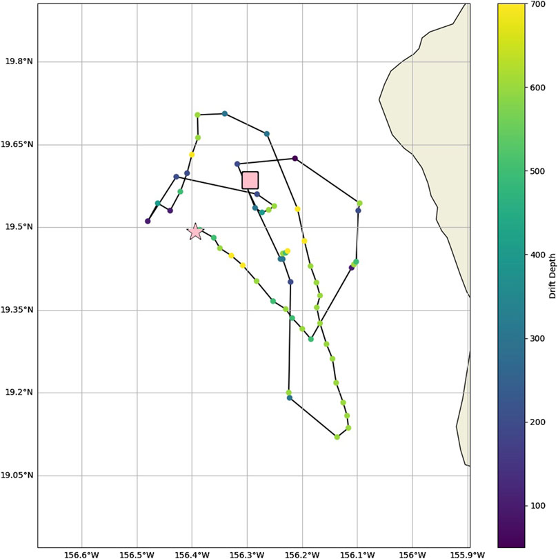
Figure 3. Example of Navigability Study for a Kona deployment. Pink star represents deployment location, pink square represents the recovery location, black line represents the HyperNav trajectory, colored dots represent the calculated ideal drift depth, beige shading represents land.

Figure 4

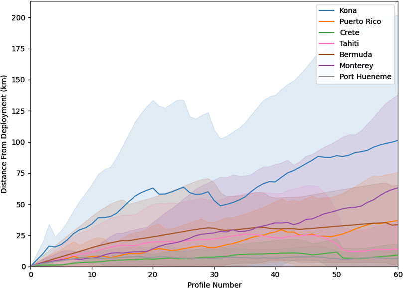
Figure 4. Aggregated estimates of site navigability (Section 4.3.2) for 60 profiles at Puerto Rico (orange), Hawaii (blue), Port Hueneme (grey), Monterey (purple), Bermuda (brown), Crete (green), and Tahiti (pink). Solid lines represent the mean estimate of displacement away from the starting point by profile number, shading represents the standard deviation of 20 controlability runs. Smaller distances from the deployment point indicate that the sites have a navigable current structure; larger distances indicate that the site is un-navigable. Sites that exceed a displacement of 20 km are anticipated to need a small boat repostioning as shown in Table 1.

Unnavigable sites can still have utility for the program if the SVC match-up probability is sufficiently high, but the expense of additional boat time to reposition floats needed to be quantified. Sites where the average float trajectories exceeded a distance of 20 km from the deployment site were deemed to require a small boat repositioning.

Our choice for quantifying site navigability (Figure 4) includes increased logistical expense in locations where we expect to require additional small boat charters to reposition floats that are uncontrollably advected a substantial (greater than 20 km) distance from their deployment site. Based on the rate that distance from the deployment site uncontrollably increased, the sites considered can be grouped into three classifications: sites that are navigable and will not require additional repositioning (Port Hueneme, Crete, Tahiti), sites that are semi-navigable and will likely require one repositioning (Monterey, Bermuda, Puerto Rico), and sites that are unreliably-navigable and will require 2 or more repositionings (Hawaii). The maximum standard deviation of distance from deployment location over the simulations at each site was as much as 84% of the maximum mean distance from deployment location, implying large variability among simulations. Of these classifications, we anticipate navigable sites to not need repositioning and only require 2 small boat charters (one for deployment and one for recovery), semi-navigable sites to need 3 small boat charters (one additional charter for repositioning), and unreliably navigable locations to require 4 or more small boat charters for frequent repositionings. These increased expenses are found in the “Boat Modifier” column of Table 1.

5 Prediction of potential match-ups

To estimate the number of seasonal match-ups at each deployment site, we interrogated the SVC probability maps in Section 4.1 at the deployment locations in Section 4.3.2 (Figure 5). The seasonal estimate of the number of match-ups was combined with our estimates for logistical expenses (Section 4.2) informed by the navigability tests (Section 4.3.2) to estimate the seasonally varying cost per SVC match-up at each deployment site. Finally, the cost of each SVC match-up was calculated by dividing the costs (Table 1) associated with each deployment site (Figure 6) by the aggregated mean of likely match-ups at each month.

Figure 5

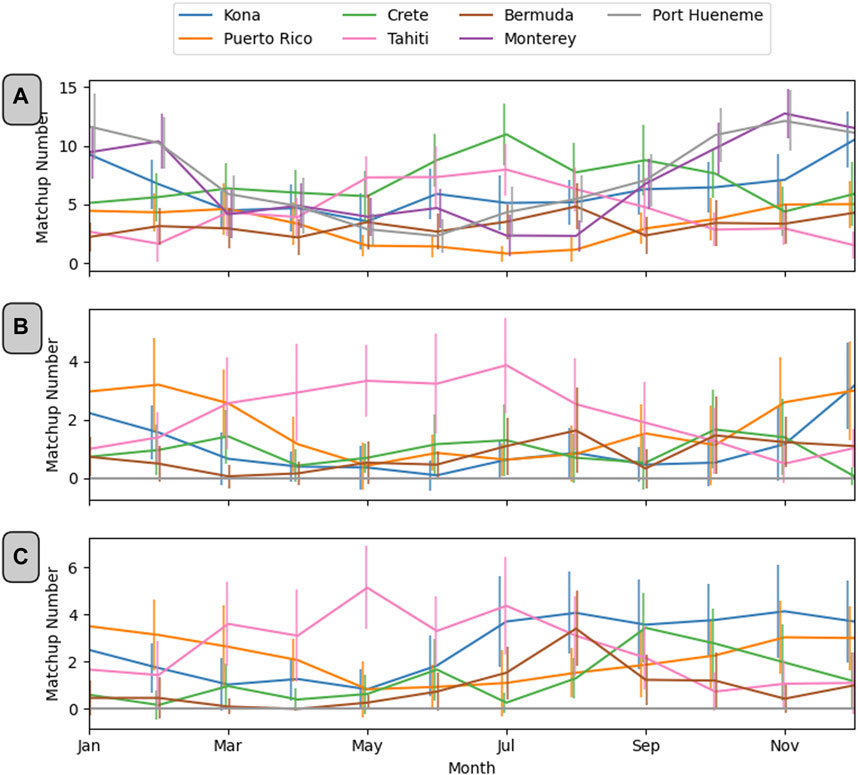
Figure 5. Seasonal estimate of number of match-ups recorded by HyperNav system at each site. Colored lines represent estimated seasonal mean (horizontal) and standard deviation (vertical) of match-ups at Port Hueneme (grey), Kona (blue), Crete (green), Tahiti (pink), Puerto Rico (orange), Monterey (purple), and Bermuda (brown) using the clearsky criterion (panel (A)), the Zibordi and Mélin (2017) criteria (panel (B)), and the criteria described in Section 2 (panel (C)).

Figure 6

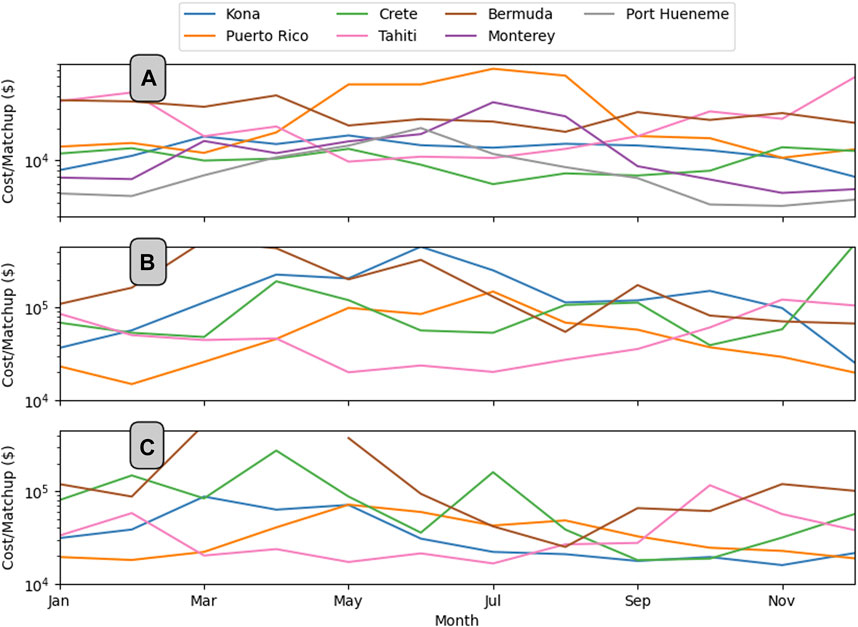
Figure 6. Seasonal USD ($) cost per match-up for monthlong deployment at each considered deployment site for (A) clear sky criterion described in Section 4.1, (B) Zibordi and Mélin (2017) criteria, and (C) match-up criteria described in Section 2. Colored lines represent the mean cost of Port Hueneme (grey), Kona (blue), Crete (green), Tahiti (pink), Puerto Rico (orange), Monterey (purple), and Bermuda (brown) deployment sites.

The stricter SVC match-up criteria of Zibordi and Mélin (2017) and that described in (Section 2) as compared with the clear sky criteria suitable for validation match-ups unsurprisingly resulted in far fewer SVC match-ups, which increased SVC match-up cost by approximately an order of magnitude (Figures 6B, C). Additionally, because of sub-mesoscale coastal processes, Monterey and Port Hueneme have high spatial variability of $R_{rs}$ and were unsuitable for SVC match-ups (Figures 5B, C); however, because of a highly retentive circulation, efficient logistics (low travel and transport costs), and a high likelihood of cloudless days Figure 5A Port Hueneme outperforms other sites half the year (fall and winter) in cost per clear sky match-up. Crete outperforms other sites in clear sky matchups for the other half of the year (spring and summer) (Figure 6A). It should be noted that we have found evidence for strongly recirculating, bathymetry-controlled, retentive eddies at both the Crete and Port Hueneme sites, and these locations should be considered for future observations so long as the clear sky SVC match-up criteria have utility for validating future ocean color products (Figure 4). There exist 2 distinct phases to the seasonal cycle of clear sky match-up costing: cost of match-ups in North American sites (Monterey, Port Hueneme, Kona, Puerto Rico) all peaking in the summer months and reaching minima in the winter; Tahiti, Bermuda, and Crete had opposite phasing with the price per match-up peaking during the winter months and reaching a minima in the summer. The minimal cost for clear sky match-up of all sites considered were January deployments in Port Hueneme with a cost per match-up of $\approx$ $4,000; the absolute maxima was June deployments in Puerto Rico with a cost per match-up of $\approx$ $80,000.

The Zibordi and Mélin (2017) criteria described in Section 2 includes more atmospheric and oceanic processes; therefore, the resulting seasonal distributions are more complex. The seasonal phasing of the Zibordi and Mélin (2017) criteria has similarities with the clear sky criteria in that the cost of match-ups of sites excluding Crete and Bermuda peak follow a predictable hemispheric seasonality. Bermuda and Crete do not exhibit an obvious seasonal signal. The absolute cost minima per match-up is found to be $\approx$ $15,000–found in February, Puerto Rico deployments and May, Tahiti deployments; The absolute average cost maxima is a March, Bermuda deployment, where the cost per match-up is $\approx$ $430,000 (Figure 6B).

Finally, the seasonality of the criteria described in Section 4.1 is similar to both the clear sky and Zibordi and Mélin (2017) criteria, except that it is phase shifted earlier in the year, approximately 3 months. The minimal cost per match-up was May deployments in Tahiti of $\approx$ $14,000. The most expensive was April deployments in Bermuda, where no match-ups were expected (Figure 6C).

6 Discussion

The selection criterion primarily discussed in this publication is cost (Figure 6). The HyperNav program has the additional goals of providing as many SVC match-ups after the PACE launch as possible and providing observations in independent and varying optical regimes. Like many optimizations applied to the real world, simplifying assumptions were made, and our conclusions must be considered in this context. In addition to cost considerations, it is essential to highlight the significance of all considered sites in providing a substantial number of match-ups for validation purposes. For instance, during the winter months, deployments from Port Hueneme in the Southern California Bight could potentially yield over 10 match-ups per month, showcasing diverse environmental conditions for validation. It is noteworthy that deploying at Port Hueneme and Monterey is not suitable for SVC due primarily to ocean variability. However, deploying HyperNav systems at the other sites would benefit both SVC and validation activities. Thus, site selection may consider optimizing both types of activities.

The navigability test, although illuminating, makes fundamental assumptions about the skill of models and the inherent risks of operations. The placement of mesoscale features in many models (including reanalysis) is commonly wrong. However, we assume the looser condition that the general structure of mesoscale statistics is accurate. The degree to which this condition holds is unclear and is likely regionally specific because the spatial resolutions and model formulations vary by site. Another assumption fundamental to the navigability test is that the predictive models have perfect skill and that while floats are deployed in the field, we can best use ocean circulation predictions. For similar reasons, a given model’s predictive skill is unclear and likely regionally specific. Finally, sites where floats are advected uncontrollably away from the deployment location have an inherent and increased risk of becoming lost or damaged. Floats can quickly travel (Figure 4) too far away from local ports to be recovered by small boats and risk never being recovered. Float repositioning also has its own risks. A float drifting at its park depth is far safer than on the rolling deck of a small boat where delicate sensors can be damaged. These risks are not factored into these calculations and should be further studied.

The top three sites considered (Kona, Puerto Rico, and Tahiti) are located within an absolute latitude band of 19.5$°$ to 17.5$°$. These locations are objectively most suitable for the Zibordi and Mélin criteria and would be the three recommendations if cost optimization were the only criteria considered. However, in the context of a global observing system, restricting the SVC match-up sites to such a limited range of latitudes, during seasons conducive for SVC match-up, may bias the satellite calibration (Bisson et al., 2021). The diversity of observing sites may be an important factor in an unbiased SVC match-up array and is something that the optimization process presented here does not capture. However, the substantial seasonal cycle of SVC match-up cost (Figure 6) highlights the advantage of the flexibility of the HyperNav system. With a small logistical footprint, HyperNav systems can be redeployed globally to anticipate the atmospheric and oceanic conditions that are favorable to SVC match-up and for validation match-up.

Community consensus and guidance do not exist for which SVC match-up criteria should be used for PACE. This is problematic from an operational perspective because, while similarities exist between the Zibordi and Mélin (2017) and Section 2 criteria, there are also substantial differences (Figure 7) and optimizing around unclear SVC match-up criteria could cause sub-optimal deployment choices. These differences are most pronounced for the expected value of fall Crete and summer and fall Kona match-ups. For Crete, this may be due to a reduction of dust storms, which are more common during spring and summer, seasons of increased atmospheric instability over North Africa. For Kona, the Zibordi and Mélin (2017) criteria may eliminate situations of small, non-absorbing aerosols. The Big Island of Hawaii is subjected to volcanic eruptions, generating non-absorbing sulfate aerosols with $\alpha >1$ that are eliminated by the Zibordi and Mélin (2017) criterion of $\alpha <1$. Of the sites considered, Section 2 criteria are more permissive, allowing 36 more annual match-ups per year at the sites considered - half of these coming from increased match-ups in Kona.

Figure 7

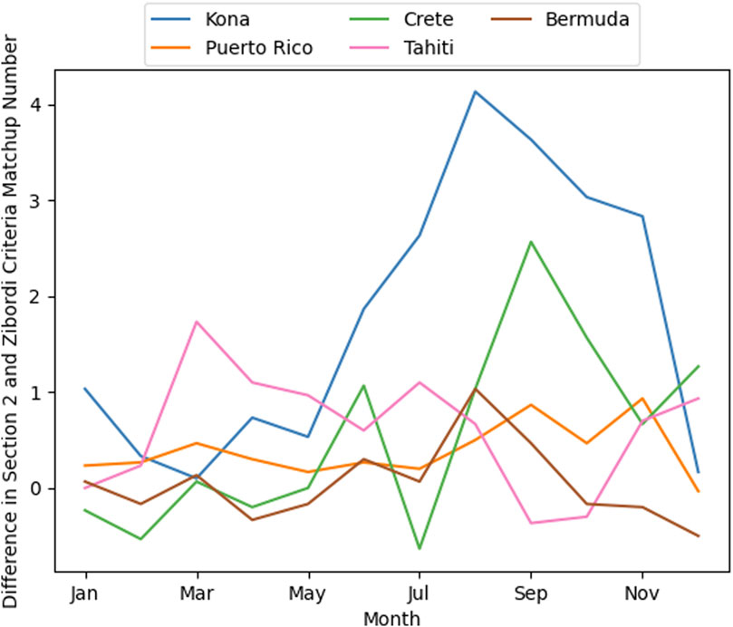
Figure 7. Seasonal match-up difference between criteria described in Section 2; Zibordi and Mélin (2017) criteria. Colored lines represent the difference in the estimated seasonal number of match-ups at Kona (blue), Puerto Rico (orange), Tahiti (pink), Crete (green), Bermuda (brown), Monterey (purple), and Port Hueneme (grey). Positive number means that Section 2 criteria allows more match-ups than the Zibordi and Mélin (2017) criteria.

Despite this lack of consensus, preliminary HyperNav deployments have been initiated for system development and satellite validation purposes, spanning both the pre and post PACE eras. Table 2 presents a subset of the 15 most successful deployments from November 2017 to the present. Data from these ongoing deployments are integrated in near real-time into the NASA PACE SVC effort, highlighting the flexibility and effectiveness of the HyperNav system.

Table 2

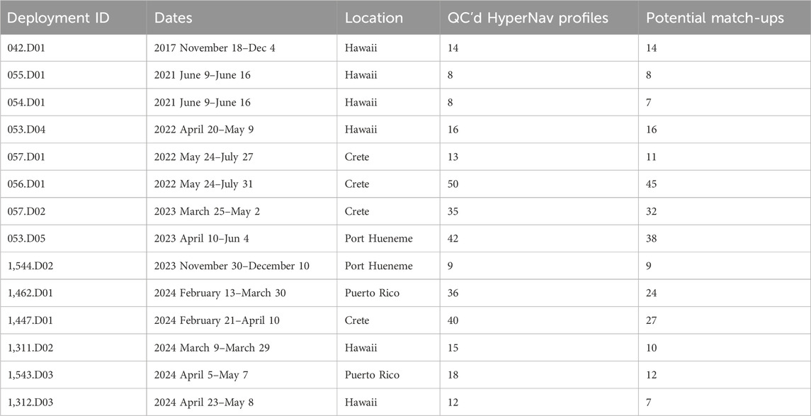
Table 2. HyperNav project deployments as of 9 May 2024 with more than 8 quality controlled (QC’d) HyperNav profiles. During initial test deployments, HyperNav system was not turned on or functioning properly for all profiles. Potential match-ups are QC’d HyperNav profiles that satisfy internal system checks and have spectra broadly similar to clear sky models. These data can be accessed from the HyperNav website (https://misclab.umeoce.maine.edu/HyperNAV/).

7 Conclusion

A methodology for selecting cost-efficient System Vicarious Calibration (SVC) and validation match-up sites using the HyperNav system has been developed. This versatile methodology is applicable across various locations. Seven specific sites were examined: Puerto Rico, Kona, Port Hueneme, Monterey Bay, Bermuda, Crete, and Tahiti. Evaluation based on three primary criteria, i.e., number of SVC match-ups, logistics, and navigability, revealed substantial differences among the sites and underscored the need for a flexible selection approach. Notably, while Port Hueneme and Monterey did not meet SVC match-up criteria, they emerged as leading sites for validation due to their abundance of clear sky days and diverse environmental conditions. For instance, during the winter months, deployments from Port Hueneme in the Southern California Bight could potentially yield over 10 validation match-ups monthly (Figure 6). Deploying HyperNav systems at the other sites would benefit both SVC and validation activities, highlighting the importance of optimizing both types of activities in site selection processes. The navigability of sites was categorized into three groups: navigable (Crete, Port Hueneme, and Tahiti), semi-navigable (Bermuda, Monterey, and Puerto Rico), and un-navigable (Kona). Semi-navigable or un-navigable sites may require additional small boat charters for float repositioning, and these costs were integrated into the logistics model (Table 1). Based on the evaluation criteria, Kona, Puerto Rico, and Tahiti emerge as promising sites for SVC match-ups.

Data availability statement

The datasets presented in this study can be found in online repositories. The names of the repository/repositories and accession number(s) can be found below: https://github.com/Chamberpain/HyperNav.

Author contributions

PC: Writing–original draft, methodology. RF: Writing–original draft, conceptualization. JT: Writing–original draft, formal analysis. MM: Writing–review and editing. AB: Funding acquisition, Writing–review and editing, EB: Writing–review and editing, methodology, NH: Writing–review and editing, data curation. CO: Writing–review and editing, Project administration.

Funding

The author(s) declare that financial support was received for the research, authorship, and/or publication of this article. All authors acknowledge support from HyperNav project under NASA awards 80GSFC20C0101 and 180GSFC22CA050.

Acknowledgments

We thank A. Banks and N. Spyridakis of the Helenic Center for Marine Research in Crete for valuable assistance in science, logistics and deployments off Crete. William Hernandez from Environmental Mapping consultants and Fernando Gilbes Santaella and Roy Armstrong from University of Puerto Rico for valuable assistance in science, logistics, and deployments off Puerto Rico. We also thank Neil Davies and the staff of the Gump Station for valuable assistance with deployments off Tahiti. We also thank two reviewers for their helpful comments and suggestions.

Conflict of interest

The authors declare that the research was conducted in the absence of any commercial or financial relationships that could be construed as a potential conflict of interest.

The author(s) declared that they were an editorial board member of Frontiers, at the time of submission. This had no impact on the peer review process and the final decision.

Publisher’s note

All claims expressed in this article are solely those of the authors and do not necessarily represent those of their affiliated organizations, or those of the publisher, the editors and the reviewers. Any product that may be evaluated in this article, or claim that may be made by its manufacturer, is not guaranteed or endorsed by the publisher.

References

Ahmad, Z., Franz, B. A., McClain, C. R., Kwiatkowska, E. J., Werdell, J., Shettle, E. P., et al. (2010). New aerosol models for the retrieval of aerosol optical thickness and normalized water-leaving radiances from the seawifs and modis sensors over coastal regions and open oceans. Appl. Opt. 49, 5545–5560. doi:10.1364/ao.49.005545

PubMed Abstract | CrossRef Full Text | Google Scholar

Antoine, D., Chami, M., Claustre, H., d’Ortenzio, F., Morel, A., Bécu, G., et al. (2006). BOUSSOLE: a joint CNRS-INSU, ESA, CNES, and NASA ocean color calibration and validation activity. Tech. Rep.

Google Scholar

Antoine, D., Guevel, P., Deste, J.-F., Becu, G., Louis, F., Scott, A. J., et al. (2008). The “boussole” buoy—a new transparent-to-swell taut mooring dedicated to marine optics: design, tests, and performance at sea. J. Atmos. Ocean. Technol. 25, 968–989. doi:10.1175/2007jtecho563.1

CrossRef Full Text | Google Scholar

Bailey, S. W., and Werdell, P. J. (2006). A multi-sensor approach for the on-orbit validation of ocean color satellite data products. Remote Sens. Environ. 102, 12–23. doi:10.1016/j.rse.2006.01.015

CrossRef Full Text | Google Scholar

Barnard, A., Van Dommelen, R., Boss, E., Plache, B., Simontov, V., Orrico, C., et al. (2022). A new paradigm for ocean color satellite calibration and validation: accurate measurements of hyperspectral water leaving radiance from autonomous profiling floats (hypernav). Authorea Prepr.

Google Scholar

Barnard, A., Boss, E., Haëntjens, N., Orrico, C., Frouin, R., Tan, J., et al. (2024a). Design and verification of a highly accurate in-situ hyperspectral radiometric measurement system (HyperNav). Frontiers in Remote Sensing. 5, 1369769. doi:10.3389/frsen.2024.1369769

CrossRef Full Text | Google Scholar

Barnard, A. E., Boss, N., Haëntjens, C., Chamberlain, R., Frouin, M., Tan, J., et al. (2024b). A float-based ocean color vicarious calibration program. Frontiers in Remote Sensing.

Google Scholar

Brewin, J., Sathyendranath, S., Kulk, G., Rio, M., Concha, J., Bell, T., et al. (2023). Ocean carbon from space: Current status and priorities for the next decade. Earth-science reviews 240 (03), 104386. doi:10.1016/j.earscirev.2023.104386

CrossRef Full Text | Google Scholar

Bisson, K., Boss, E., Werdell, P. J., Ibrahim, A., Frouin, R., and Behrenfeld, M. (2021). Seasonal bias in global ocean color observations. Appl. Opt. 60, 6978–6988. doi:10.1364/ao.426137

PubMed Abstract | CrossRef Full Text | Google Scholar

Campbell, J. W., Blaisdell, J. M., and Darzi, M. (1996). Level-3 sea wifs data products: spatial and temporal binning algorithms. Oceanogr. Lit. Rev. 9, 952.

Google Scholar

Chamberlain, P., Talley, L. D., Mazloff, M., Van Sebille, E., Gille, S. T., Tucker, T., et al. (2023). Using existing argo trajectories to statistically predict future float positions with a transition matrix. J. Atmos. Ocean. Technol. 40, 1083–1103. doi:10.1175/jtech-d-22-0070.1

CrossRef Full Text | Google Scholar

Chassignet, E. P., Hurlburt, H. E., Metzger, E. J., Smedstad, O. M., Cummings, J. A., Halliwell, G. R., et al. (2009). Us godae: global ocean prediction with the hybrid coordinate ocean model (hycom). Oceanography 22, 64–75. doi:10.5670/oceanog.2009.39

CrossRef Full Text | Google Scholar

Clark, D., Gordon, H., Voss, K., Ge, Y., Broenkow, W., and Trees, C. (1997). Validation of atmospheric correction over the oceans. J. Geophys. Res. Atmos. 102, 17209–17217. doi:10.1029/96jd03345

CrossRef Full Text | Google Scholar

Clark, D. K., Yarbrough, M. A., Feinholz, M., Flora, S., Broenkow, W., Kim, Y. S., et al. (2003). Moby, a radiometric buoy for performance monitoring and vicarious calibration of satellite ocean color sensors: measurement and data analysis protocols. Ocean Opt. Protoc. Satell. Ocean Color Sens. Validation 6.

Google Scholar

Cummings, J. A., and Smedstad, O. M. (2014). Ocean data impacts in global hycom. J. Atmos. Ocean. Technol. 31, 1771–1791. doi:10.1175/jtech-d-14-00011.1

CrossRef Full Text | Google Scholar

Dubovik, O., Holben, B., Eck, T. F., Smirnov, A., Kaufman, Y. J., King, M. D., et al. (2002). Variability of absorption and optical properties of key aerosol types observed in worldwide locations. J. Atmos. Sci. 59, 590–608. doi:10.1175/1520-0469(2002)059<0590:voaaop>2.0.co;2

CrossRef Full Text | Google Scholar

Escudier, R., Clementi, E., Cipollone, A., Pistoia, J., Drudi, M., Grandi, A., et al. (2021). A high resolution reanalysis for the mediterranean sea. Front. Earth Sci. 9, 702285. doi:10.3389/feart.2021.702285

CrossRef Full Text | Google Scholar

Evans, R. H., and Gordon, H. R. (1994). Coastal zone color scanner “system calibration”: a retrospective examination. J. Geophys. Res. Oceans 99, 7293–7307. doi:10.1029/93jc02151

CrossRef Full Text | Google Scholar

Fougnie, B., Deschamps, P.-Y., and Frouin, R. (1999). Vicarious calibration of the polder ocean color spectral bands using in situ measurements. IEEE Trans. geoscience remote Sens. 37, 1567–1574. doi:10.1109/36.763267

CrossRef Full Text | Google Scholar

Fougnie, B., Henry, P., Morel, A., Antoine, D., and Montagner, F. (2002). Identification and characterization of stable homogeneous oceanic zones: climatology and impact on in-flight calibration of space sensor over Rayleigh scattering. Ocean. Opt. XVI, 18–22. Santa Fe, NM.

Google Scholar

Fougnie, B., Llido, J., Gross-Colzy, L., Henry, P., and Blumstein, D. (2010). Climatology of oceanic zones suitable for in-flight calibration of space sensors. Earth Obs. Syst. XV (SPIE) 7807, 215–225.

CrossRef Full Text | Google Scholar

Franz, B. A., Bailey, S. W., Werdell, P. J., and McClain, C. R. (2007). Sensor-independent approach to the vicarious calibration of satellite ocean color radiometry. Appl. Opt. 46, 5068–5082. doi:10.1364/ao.46.005068

PubMed Abstract | CrossRef Full Text | Google Scholar

Frouin, R., et al. (2013). In-flight calibration of satellite ocean-colour sensors. Canada: International Ocean-Colour Coordinating Group.

Google Scholar

Frouin, R. J., Franz, B. A., Ibrahim, A., Knobelspiesse, K., Ahmad, Z., Cairns, B., et al. (2019). Atmospheric correction of satellite ocean-color imagery during the pace era. Front. Earth Sci. 7, 145. doi:10.3389/feart.2019.00145

CrossRef Full Text | Google Scholar

Gilerson, A., Herrera-Estrella, E., Foster, R., Agagliate, J., Hu, C., Ibrahim, A., et al. (2022). Determining the primary sources of uncertainty in retrieval of marine remote sensing reflectance from satellite ocean color sensors. Front. Remote Sens. 3. doi:10.3389/frsen.2022.857530

CrossRef Full Text | Google Scholar

González Santana, A., Oosterbaan, M., Clavelle, T., Maze, G., Notarstefano, G., Poffa, N., et al. (2023). “Analysis of the global shipping traffic for the feasibility of a structural recovery program of argo floats,” in XXVIII general assembly of the international union of geodesy and geophysics (IUGG) (GFZ German Research Centre for Geosciences).

Google Scholar

Gordon, H. R. (1987). Calibration requirements and methodology for remote sensors viewing the ocean in the visible. Remote Sens. Environ. 22, 103–126. doi:10.1016/0034-4257(87)90029-0

CrossRef Full Text | Google Scholar

Gordon, H. R. (1998). In-orbit calibration strategy for ocean color sensors. Remote Sens. Environ. 63, 265–278. doi:10.1016/s0034-4257(97)00163-6

CrossRef Full Text | Google Scholar

Groom, S., Sathyendranath, S., Ban, Y., Bernard, S., Brewin, R., Brotas, V., et al. (2019). Satellite ocean colour: current status and future perspective. Front. Mar. Sci. 6, 1–30. doi:10.3389/fmars.2019.00485

PubMed Abstract | CrossRef Full Text | Google Scholar

Johnson, B., Zibordi, G., Kwiatkowska, E., Voss, K., Melin, F., Antoine, D., et al. (2024). System Vicarious Calibration requirements for satellite ocean colour missions targeting climate and global long-term operational applications. Available at: https://tsapps.nist.gov/publication/get_pdf.cfm?pub_id=957358 (Accessed July 5, 2024).

Google Scholar

Kwiatkowska, E., Babu, K. N., Bojkov, B., Dessailly, D., Gilmore, R., Goryl, P., et al. (2022). Conclusions of the review of candidate locations for copernicus ocean colour system vicarious calibration infrastructure. Darmstadt, Germany: EUMETSAT.

Google Scholar

Lange, M., and van Sebille, E. (2017). Parcels v0. 9: prototyping a Lagrangian ocean analysis framework for the petascale age. Geosci. Model Dev. 10, 4175–4186. doi:10.5194/gmd-10-4175-2017

CrossRef Full Text | Google Scholar

McClain, C. R., Meister, G., et al. (2012). Mission requirements for future ocean-colour sensors. Dartmouth, NS, Canada: International Ocean Colour Coordinating Group (IOCCG).

Google Scholar

Miller, R. N. (1990). Tropical data assimilation experiments with simulated data: the impact of the tropical ocean and global atmosphere thermal array for the ocean. J. Geophys. Res. Oceans 95, 11461–11482. doi:10.1029/jc095ic07p11461

CrossRef Full Text | Google Scholar

Morel, A., and Prieur, L. (1977). Analysis of variations in ocean color 1. Limnol. Oceanogr. 22, 709–722. doi:10.4319/lo.1977.22.4.0709

CrossRef Full Text | Google Scholar

Parrington, J. R., Zoller, W. H., and Aras, N. K. (1983). Asian dust: seasonal transport to the Hawaiian islands. Science 220, 195–197. doi:10.1126/science.220.4593.195

PubMed Abstract | CrossRef Full Text | Google Scholar

Powell, B. S. (2018). Regional ocean modeling system (roms): main Hawaiian islands: reanalysis. Pac. Isl. Ocean. Obs. Syst. 27.

Google Scholar

Roemmich, D., Alford, M. H., Claustre, H., Johnson, K., King, B., Moum, J., et al. (2019). On the future of Argo: a global, full-depth, multi-disciplinary array. Front. Mar. Sci. 6, 439. doi:10.3389/fmars.2019.00439

CrossRef Full Text | Google Scholar

Santer, R., and Schmechtig, C. (2000). Adjacency effects on water surfaces: primary scattering approximation and sensitivity study. Appl. Opt. 39, 361–375.

PubMed Abstract | CrossRef Full Text | Google Scholar

Servain, J., Busalacchi, A. J., McPhaden, M. J., Moura, A. D., Reverdin, G., Vianna, M., et al. (1998). A pilot research moored array in the tropical atlantic (pirata). Bull. Am. Meteorological Soc. 79, 2019–2031. doi:10.1175/1520-0477(1998)079<2019:aprmai>2.0.co;2

CrossRef Full Text | Google Scholar

Siiriä, S., Roiha, P., Tuomi, L., Purokoski, T., Haavisto, N., and Alenius, P. (2019). Applying area-locked, shallow water argo floats in baltic sea monitoring. J. Operational Oceanogr. 12, 58–72. doi:10.1080/1755876x.2018.1544783

CrossRef Full Text | Google Scholar

Valente, A., Sathyendranath, S., Brotas, V., Groom, S., Grant, M., Taberner, M., et al. (2016). A compilation of global bio-optical in situ data for ocean-colour satellite applications. Earth Syst. Sci. Data 8, 235–252. doi:10.5194/essd-8-235-2016

CrossRef Full Text | Google Scholar

Wallcraft, A., Metzger, E., and Carroll, S. (2009). Software design description for the hybrid coordinate ocean model (hycom) version 2.2. Nav. Res. Laboratory, 13–15.

CrossRef Full Text | Google Scholar

Werdell, P. J., Behrenfeld, M. J., Bontempi, P. S., Boss, E., Cairns, B., Davis, G. T., et al. (2019). The plankton, aerosol, cloud, ocean ecosystem mission: status, science, advances. Bull. Am. Meteorological Soc. 100, 1775–1794. doi:10.1175/BAMS-D-18-0056.1

CrossRef Full Text | Google Scholar

Wong, A. P., Wijffels, S. E., Riser, S. C., Pouliquen, S., Hosoda, S., Roemmich, D., et al. (2020). Argo data 1999–2019: two million temperature-salinity profiles and subsurface velocity observations from a global array of profiling floats. Front. Mar. Sci. 7, 700. doi:10.3389/fmars.2020.00700

CrossRef Full Text | Google Scholar

Zibordi, G., and Mélin, F. (2017). An evaluation of marine regions relevant for ocean color system vicarious calibration. Remote Sens. Environ. 190, 122–136. doi:10.1016/j.rse.2016.11.020

PubMed Abstract | CrossRef Full Text | Google Scholar

Zibordi, G., Mélin, F., Voss, K. J., Johnson, B. C., Franz, B. A., Kwiatkowska, E., et al. (2015). System vicarious calibration for ocean color climate change applications: requirements for in situ data. Remote Sens. Environ. 159, 361–369. doi:10.1016/j.rse.2014.12.015

CrossRef Full Text | Google Scholar